
Содержание
- Create a Data Model in Excel
- Getting started
- Create Relationships between your tables
- Use a Data Model to create a PivotTable or PivotChart
- Add existing, unrelated data to a Data Model
- Adding data to a Power Pivot table
- Need more help?
- How to create a CSV file
- Example spreadsheet data
- Creating a CSV file
- Notepad (or any text editor)
- Microsoft Excel
- OpenOffice Calc
- Google Docs
Create a Data Model in Excel
A Data Model allows you to integrate data from multiple tables, effectively building a relational data source inside an Excel workbook. Within Excel, Data Models are used transparently, providing tabular data used in PivotTables and PivotCharts. A Data Model is visualized as a collection of tables in a Field List, and most of the time, you’ll never even know it’s there.
Before you can start working with the Data Model, you need to get some data. For that we’ll use the Get & Transform (Power Query) experience, so you might want to take a step back and watch a video, or follow our learning guide on Get & Transform and Power Pivot.
Excel 2016 & Excel for Microsoft 365 — Power Pivot is included in the Ribbon.
Excel 2013 — Power Pivot is part of the Office Professional Plus edition of Excel 2013, but is not enabled by default. Learn more about starting the Power Pivot add-in for Excel 2013.
Excel 2016 & Excel for Microsoft 365 — Get & Transform (Power Query) has been integrated with Excel on the Data tab.
Excel 2013 — Power Query is an add-in that’s included with Excel, but needs to be activated. Go to File > Options > Add-Ins, then in the Manage drop-down at the bottom of the pane, select COM Add-Ins > Go. Check Microsoft Power Query for Excel, then OK to activate it. A Power Query tab will be added to the ribbon.
Excel 2010 — Download and install the Power Query add-in.. Once activated, a Power Query tab will be added to the ribbon.
Getting started
First, you need to get some data.
In Excel 2016, and Excel for Microsoft 365, use Data > Get & Transform Data > Get Data to import data from any number of external data sources, such as a text file, Excel workbook, website, Microsoft Access, SQL Server, or another relational database that contains multiple related tables.
In Excel 2013 and 2010, go to Power Query > Get External Data, and select your data source.
Excel prompts you to select a table. If you want to get multiple tables from the same data source, check the Enable selection of multiple tables option. When you select multiple tables, Excel automatically creates a Data Model for you.
Note: For these examples, we’re using an Excel workbook with fictional student details on classes and grades. You can download our Student Data Model sample workbook, and follow along. You can also download a version with a completed Data Model..

Select one or more tables, then click Load.
If you need to edit the source data, you can choose the Edit option. For more details see: Introduction to the Query Editor (Power Query).
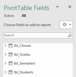
You now have a Data Model that contains all of the tables you imported, and they will be displayed in the PivotTable Field List.
Models are created implicitly when you import two or more tables simultaneously in Excel.
Models are created explicitly when you use the Power Pivot add-in to import data. In the add-in, the model is represented in a tabbed layout similar to Excel, where each tab contains tabular data. See Get data using the Power Pivot add-into learn the basics of data import using a SQL Server database.
A model can contain a single table. To create a model based on just one table, select the table and click Add to Data Model in Power Pivot. You might do this if you want to use Power Pivot features, such as filtered datasets, calculated columns, calculated fields, KPIs, and hierarchies.
Table relationships can be created automatically if you import related tables that have primary and foreign key relationships. Excel can usually use the imported relationship information as the basis for table relationships in the Data Model.
For tips on how to reduce the size of a data model, see Create a memory-efficient Data Model using Excel and Power Pivot.
Tip: How can you tell if your workbook has a Data Model? Go to Power Pivot > Manage. If you see worksheet-like data, then a model exists. See: Find out which data sources are used in a workbook data model to learn more.
Create Relationships between your tables
The next step is to create relationships between your tables, so you can pull data from any of them. Each table needs to have a primary key, or unique field identifier, like Student ID, or Class number. The easiest way is to drag and drop those fields to connect them in Power Pivot’s Diagram View.
Go to Power Pivot > Manage.
On the Home tab, select Diagram View.
All of your imported tables will be displayed, and you might want to take some time to resize them depending on how many fields each one has.
Next, drag the primary key field from one table to the next. The following example is the Diagram View of our student tables:
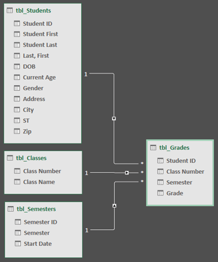
We’ve created the following links:
tbl_Students | Student ID > tbl_Grades | Student ID
In other words, drag the Student ID field from the Students table to the Student ID field in the Grades table.
tbl_Semesters | Semester ID > tbl_Grades | Semester
tbl_Classes | Class Number > tbl_Grades | Class Number
Field names don’t need to be the same in order to create a relationship, but they do need to be the same data type.
The connectors in the Diagram View have a «1» on one side, and an «*» on the other. This means that there is a one-to-many relationship between the tables, and that determines how the data is used in your PivotTables. See: Relationships between tables in a Data Model to learn more.
The connectors only indicate that there is a relationship between tables. They won’t actually show you which fields are linked to each other. To see the links, go to Power Pivot > Manage > Design > Relationships > Manage Relationships. In Excel, you can go to Data > Relationships.
Use a Data Model to create a PivotTable or PivotChart
An Excel workbook can contain only one Data Model, but that model can contain multiple tables which can be used repeatedly throughout the workbook. You can add more tables to an existing Data Model at any time.
In Power Pivot, go to Manage.
On the Home tab, select PivotTable.
Select where you want the PivotTable to be placed: a new worksheet, or the current location.
Click OK, and Excel will add an empty PivotTable with the Field List pane displayed on the right.
Next, create a PivotTable, or create a Pivot Chart. If you’ve already created relationships between the tables, you can use any of their fields in the PivotTable. We’ve already created relationships in the Student Data Model sample workbook.
Suppose you’ve imported or copied lots of data that you want to use in a model, but haven’t added it to the Data Model. Pushing new data into a model is easier than you think.
Start by selecting any cell within the data that you want to add to the model. It can be any range of data, but data formatted as an Excel table is best.
Use one of these approaches to add your data:
Click Power Pivot > Add to Data Model.
Click Insert > PivotTable, and then check Add this data to the Data Model in the Create PivotTable dialog box.
The range or table is now added to the model as a linked table. To learn more about working with linked tables in a model, see Add Data by Using Excel Linked Tables in Power Pivot.
Adding data to a Power Pivot table
In Power Pivot, you cannot add a row to a table by directly typing in a new row like you can in an Excel worksheet. But you can add rows by copying and pasting, or updating the source data and refreshing the Power Pivot model.
Need more help?
You can always ask an expert in the Excel Tech Community or get support in the Answers community.
Источник
How to create a CSV file

CSV is a simple file format used to store tabular data, such as a spreadsheet or database. Files in the CSV format can be imported to and exported from programs that store data in tables, such as Microsoft Excel or OpenOffice Calc.
CSV stands for «comma-separated values». Its data fields are often separated, or delimited, by a comma.
Example spreadsheet data
For example, let’s say you had a spreadsheet containing the following data.
| Name | Class | Dorm | Room | GPA |
|---|---|---|---|---|
| Sally Whittaker | 2018 | McCarren House | 312 | 3.75 |
| Belinda Jameson | 2017 | Cushing House | 148 | 3.52 |
| Jeff Smith | 2018 | Prescott House | 17-D | 3.20 |
| Sandy Allen | 2019 | Oliver House | 108 | 3.48 |
The above data could be represented in a CSV-formatted file as follows:
Here, the fields of data in each row are delimited with a comma and individual rows are separated by a newline.
Creating a CSV file
A CSV is a text file, so it can be created and edited using any text editor. More frequently, however, a CSV file is created by exporting (File > Export) a spreadsheet or database in the program that created it. Click a link below for the steps to create a CSV file in Notepad, Microsoft Excel, OpenOffice Calc, and Google Docs.
Notepad (or any text editor)
To create a CSV file with a text editor, first choose your favorite text editor, such as Notepad or vim, and open a new file. Then enter the text data you want the file to contain, separating each value with a comma and each row with a new line.
Save this file with the extension .csv. You can then open the file using Microsoft Excel or another spreadsheet program. It would create a table of data similar to the following:
| Title1 | Title2 | Title3 |
| one | two | three |
| example1 | example2 | example3 |
In the CSV file you created, individual fields of data were separated by commas. But what if the data itself has commas in it?
If the fields of data in your CSV file contain commas, you can protect them by enclosing those data fields in double quotes («). The commas that are part of your data are kept separate from the commas which delimit the fields themselves.
For example, let’s say that one of our text fields is a user-created description that allows commas in the description. If our data looked like this:
| Lead | Title | Phone | Notes |
| Jim Grayson | Senior Manager | (555)761-2385 | Spoke Tuesday, he’s interested |
| Prescilla Winston | Development Director | (555)218-3981 | said to call again next week |
| Melissa Potter | Head of Accounts | (555)791-3471 | Not interested, gave referral |
To retain the commas in our «Notes» column, we can enclose those fields in quotation marks. For instance:
As you can see, only the fields that contain commas are enclosed in quotes.
The same goes for newlines which may be part of your field data. Any fields containing a newline as part of its data need to be enclosed in double quotes.
If your fields contain double quotes as part of their data, the internal quotation marks need to be doubled so they can be interpreted correctly. For instance, given the following data:
| Player | Position | Nicknames | Years Active |
|---|---|---|---|
| Skippy Peterson | First Base | «Blue Dog», «The Magician» | 1908-1913 |
| Bud Grimsby | Center Field | «The Reaper», «Longneck» | 1910-1917 |
| Vic Crumb | Shortstop | «Fat Vic», «Icy Hot» | 1911-1912 |
We can represent it in a CSV file as follows:
Here, the entire data field is enclosed in quotes, and internal quotation marks are preceded (escaped by) an additional double quote.
Here are the rules of how data should be formatted in a CSV file, from the IETF’s document, RFC 4180. In these examples, «CRLF» represents a carriage return and a linefeed (which together constitute a newline).
- Each record (row of data) is to be on a separate line, delimited by a line break. For example:
The last record in the file may or may not have an ending line break. For example:
There may be an optional header line appearing as the first line of the file with the same format as normal record lines. The header contains names corresponding to the fields in the file. Also, it should contain the same number of fields as the records in the rest of the file. For example:
In the header and each record, there may be one or more fields, separated by commas. Each line should contain the same number of fields throughout the file. Spaces are considered part of a field and should not be ignored. The last field in the record must not be followed by a comma. For example:
Each field may or may not be enclosed in double quotes. If fields are not enclosed with double quotes, then double quotes may not appear inside the fields. For example:
Fields containing line breaks (CRLF), double quotes, and commas should be enclosed in double quotes. For example:
If double quotes enclose fields, then a double quote appearing inside a field must be escaped by preceding it with another double quote. For example:
Microsoft Excel
To create a CSV file using Microsoft Excel, launch Excel and then open the file you want to save in CSV format. For example, below is the data contained in our example Excel worksheet:
| Item | Cost | Sold | Profit |
|---|---|---|---|
| Keyboard | $10.00 | $16.00 | $6.00 |
| Monitor | $80.00 | $120.00 | $40.00 |
| Mouse | $5.00 | $7.00 | $2.00 |
| Total | $48.00 |
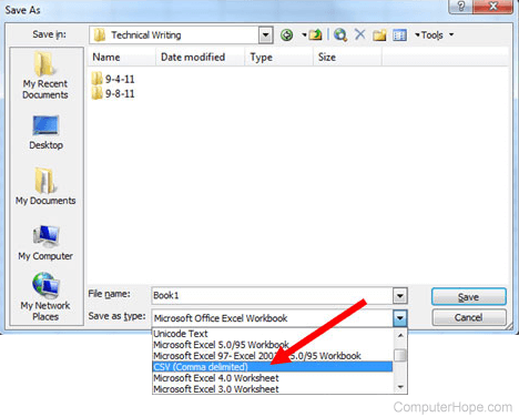
Once open, click File and choose Save As. Under Save as type, select CSV (Comma delimited) or CSV (Comma delimited) (*.csv), depending on your version of Microsoft Excel.
After you save the file, you are free to open it up in a text editor to view it or edit it manually. Its contents resemble the following:
The last row begins with two commas because the first two fields of that row were empty in our spreadsheet. Don’t delete them — the two commas are required so that the fields correspond from row to row. They cannot be omitted.
OpenOffice Calc
To create a CSV file using OpenOffice Calc, launch Calc and open the file you want to save as a CSV file. For example, below is the data contained in our example Calc worksheet.
| Item | Cost | Sold | Profit |
|---|---|---|---|
| Keyboard | $10.00 | $16.00 | $6.00 |
| Monitor | $80.00 | $120.00 | $40.00 |
| Mouse | $5.00 | $7.00 | $2.00 |
| Total | $48.00 |
Once open, click File, choose the Save As option, and for the Save as type option, select Text CSV (.csv) (*.csv).
If you were to open the CSV file in a text editor, such as Notepad, it would resemble the example below.
As in our Excel example, the two commas at the beginning of the last line make sure the fields correspond from row to row. Do not remove them!
Google Docs
Open Google Docs and open the spreadsheet file you want to save as a CSV file. Click File, Download as, and then select CSV (current sheet).
Источник
Abstract: This is the first tutorial in a series designed to get you acquainted and comfortable using Excel and its built-in data mash-up and analysis features. These tutorials build and refine an Excel workbook from scratch, build a data model, then create amazing interactive reports using Power View. The tutorials are designed to demonstrate Microsoft Business Intelligence features and capabilities in Excel, PivotTables, Power Pivot, and Power View.
Note: This article describes data models in Excel 2013. However, the same data modeling and Power Pivot features introduced in Excel 2013 also apply to Excel 2016.
In these tutorials you learn how to import and explore data in Excel, build and refine a data model using Power Pivot, and create interactive reports with Power View that you can publish, protect, and share.
The tutorials in this series are the following:
-
Import Data into Excel 2013, and Create a Data Model
-
Extend Data Model relationships using Excel, Power Pivot, and DAX
-
Create Map-based Power View Reports
-
Incorporate Internet Data, and Set Power View Report Defaults
-
Power Pivot Help
-
Create Amazing Power View Reports — Part 2
In this tutorial, you start with a blank Excel workbook.
The sections in this tutorial are the following:
-
Import data from a database
-
Import data from a spreadsheet
-
Import data using copy and paste
-
Create a relationship between imported data
-
Checkpoint and Quiz
At the end of this tutorial is a quiz you can take to test your learning.
This tutorial series uses data describing Olympic Medals, hosting countries, and various Olympic sporting events. We suggest you go through each tutorial in order. Also, tutorials use Excel 2013 with Power Pivot enabled. For more information on Excel 2013, click here. For guidance on enabling Power Pivot, click here.
Import data from a database
We start this tutorial with a blank workbook. The goal in this section is to connect to an external data source, and import that data into Excel for further analysis.
Let’s start by downloading some data from the Internet. The data describes Olympic Medals, and is a Microsoft Access database.
-
Click the following links to download files we use during this tutorial series. Download each of the four files to a location that’s easily accessible, such as Downloads or My Documents, or to a new folder you create:
> OlympicMedals.accdb Access database
> OlympicSports.xlsx Excel workbook
> Population.xlsx Excel workbook
> DiscImage_table.xlsx Excel workbook -
In Excel 2013, open a blank workbook.
-
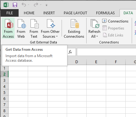
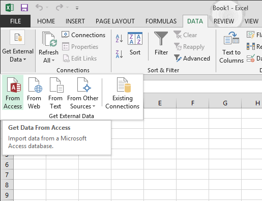
Click DATA > Get External Data > From Access. The ribbon adjusts dynamically based on the width of your workbook, so the commands on your ribbon may look slightly different from the following screens. The first screen shows the ribbon when a workbook is wide, the second image shows a workbook that has been resized to take up only a portion of the screen.

-
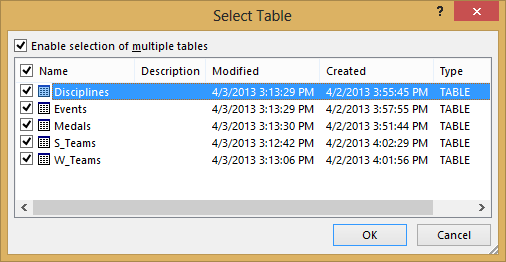
Select the OlympicMedals.accdb file you downloaded and click Open. The following Select Table window appears, displaying the tables found in the database. Tables in a database are similar to worksheets or tables in Excel. Check the Enable selection of multiple tables box, and select all the tables. Then click OK.
-
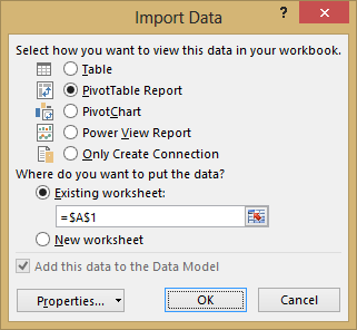
The Import Data window appears.
Note: Notice the checkbox at the bottom of the window that allows you to Add this data to the Data Model, shown in the following screen. A Data Model is created automatically when you import or work with two or more tables simultaneously. A Data Model integrates the tables, enabling extensive analysis using PivotTables, Power Pivot, and Power View. When you import tables from a database, the existing database relationships between those tables is used to create the Data Model in Excel. The Data Model is transparent in Excel, but you can view and modify it directly using the Power Pivot add-in. The Data Model is discussed in more detail later in this tutorial.
Select the PivotTable Report option, which imports the tables into Excel and prepares a PivotTable for analyzing the imported tables, and click OK.
-
Once the data is imported, a PivotTable is created using the imported tables.
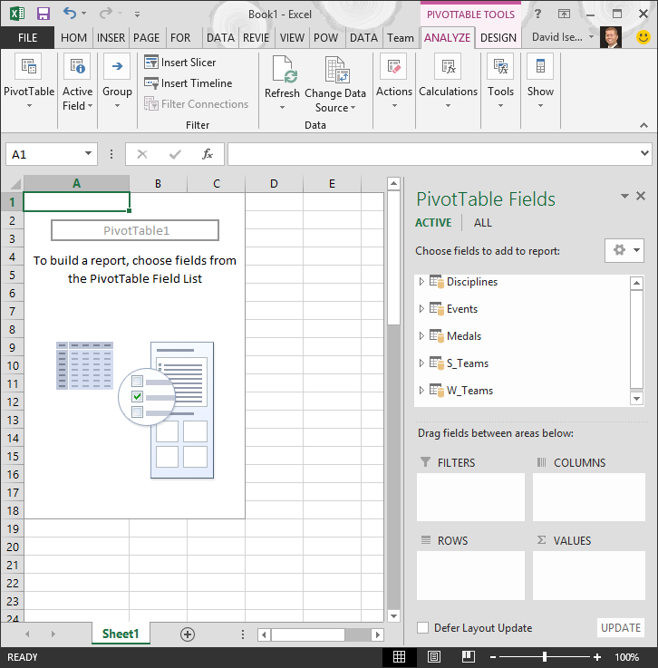
With the data imported into Excel, and the Data Model automatically created, you’re ready to explore the data.
Explore data using a PivotTable
Exploring imported data is easy using a PivotTable. In a PivotTable, you drag fields (similar to columns in Excel) from tables (like the tables you just imported from the Access database) into different areas of the PivotTable to adjust how it presents your data. A PivotTable has four areas: FILTERS, COLUMNS, ROWS, and VALUES.
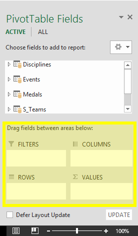
It might take some experimenting to determine which area a field should be dragged to. You can drag as many or few fields from your tables as you like, until the PivotTable presents your data how you want to see it. Feel free to explore by dragging fields into different areas of the PivotTable; the underlying data is not affected when you arrange fields in a PivotTable.
Let’s explore the Olympic Medals data in the PivotTable, starting with Olympic medalists organized by discipline, medal type, and the athlete’s country or region.
-
In PivotTable Fields, expand the Medals table by clicking the arrow beside it. Find the NOC_CountryRegion field in the expanded Medals table, and drag it to the COLUMNS area. NOC stands for National Olympic Committees, which is the organizational unit for a country or region.
-
Next, from the Disciplines table, drag Discipline to the ROWS area.
-
Let’s filter Disciplines to display only five sports: Archery, Diving, Fencing, Figure Skating, and Speed Skating. You can do this from within the PivotTable Fields area, or from the Row Labels filter in the PivotTable itself.
-
Click anywhere in the PivotTable to ensure the Excel PivotTable is selected. In the PivotTable Fields list, where the Disciplines table is expanded, hover over its Discipline field and a dropdown arrow appears to the right of the field. Click the dropdown, click (Select All)to remove all selections, then scroll down and select Archery, Diving, Fencing, Figure Skating, and Speed Skating. Click OK.
-
Or, in the Row Labels section of the PivotTable, click the dropdown next to Row Labels in the PivotTable, click (Select All) to remove all selections, then scroll down and select Archery, Diving, Fencing, Figure Skating, and Speed Skating. Click OK.
-
-
In PivotTable Fields, from the Medals table, drag Medal to the VALUES area. Since Values must be numeric, Excel automatically changes Medal to Count of Medal.
-
From the Medals table, select Medal again and drag it into the FILTERS area.
-
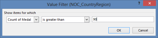
Let’s filter the PivotTable to display only those countries or regions with more than 90 total medals. Here’s how.
-
In the PivotTable, click the dropdown to the right of Column Labels.
-
Select Value Filters and select Greater Than….
-
Type 90 in the last field (on the right). Click OK.
-
Your PivotTable looks like the following screen.
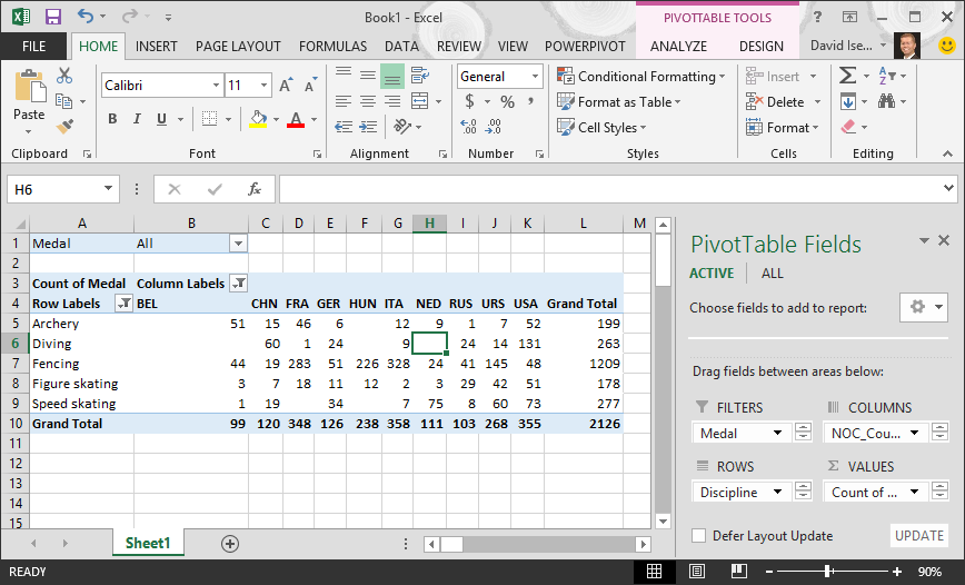
With little effort, you now have a basic PivotTable that includes fields from three different tables. What made this task so simple were the pre-existing relationships among the tables. Because table relationships existed in the source database, and because you imported all the tables in a single operation, Excel could recreate those table relationships in its Data Model.
But what if your data originates from different sources, or is imported at a later time? Typically, you can create relationships with new data based on matching columns. In the next step, you import additional tables, and learn how to create new relationships.
Import data from a spreadsheet
Now let’s import data from another source, this time from an existing workbook, then specify the relationships between our existing data and the new data. Relationships let you analyze collections of data in Excel, and create interesting and immersive visualizations from the data you import.
Let’s start by creating a blank worksheet, then import data from an Excel workbook.
-
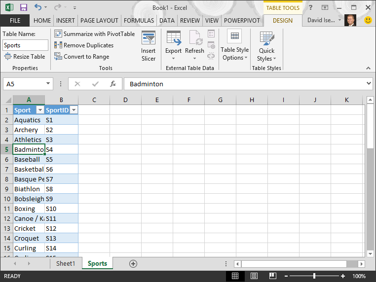
Insert a new Excel worksheet, and name it Sports.
-
Browse to the folder that contains the downloaded sample data files, and open OlympicSports.xlsx.
-
Select and copy the data in Sheet1. If you select a cell with data, such as cell A1, you can press Ctrl + A to select all adjacent data. Close the OlympicSports.xlsx workbook.
-
On the Sports worksheet, place your cursor in cell A1 and paste the data.
-
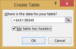
With the data still highlighted, press Ctrl + T to format the data as a table. You can also format the data as a table from the ribbon by selecting HOME > Format as Table. Since the data has headers, select My table has headers in the Create Table window that appears, as shown here.
Formatting the data as a table has many advantages. You can assign a name to a table, which makes it easy to identify. You can also establish relationships between tables, enabling exploration and analysis in PivotTables, Power Pivot, and Power View.
-
Name the table. In TABLE TOOLS > DESIGN > Properties, locate the Table Name field and type Sports. The workbook looks like the following screen.
-
Save the workbook.
Import data using copy and paste
Now that we’ve imported data from an Excel workbook, let’s import data from a table we find on a web page, or any other source from which we can copy and paste into Excel. In the following steps, you add the Olympic host cities from a table.
-
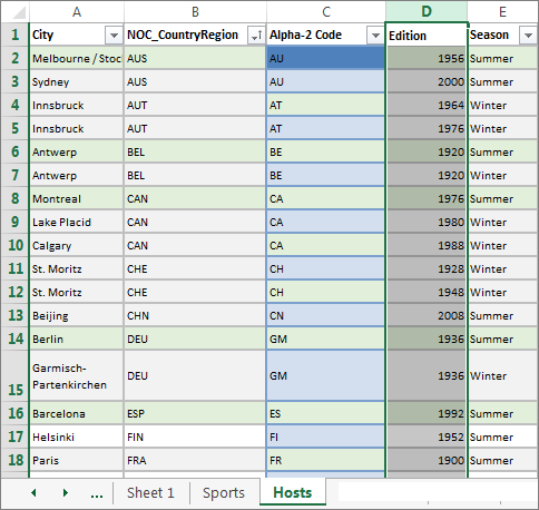
Insert a new Excel worksheet, and name it Hosts.
-
Select and copy the following table, including the table headers.
|
City |
NOC_CountryRegion |
Alpha-2 Code |
Edition |
Season |
|
Melbourne / Stockholm |
AUS |
AS |
1956 |
Summer |
|
Sydney |
AUS |
AS |
2000 |
Summer |
|
Innsbruck |
AUT |
AT |
1964 |
Winter |
|
Innsbruck |
AUT |
AT |
1976 |
Winter |
|
Antwerp |
BEL |
BE |
1920 |
Summer |
|
Antwerp |
BEL |
BE |
1920 |
Winter |
|
Montreal |
CAN |
CA |
1976 |
Summer |
|
Lake Placid |
CAN |
CA |
1980 |
Winter |
|
Calgary |
CAN |
CA |
1988 |
Winter |
|
St. Moritz |
SUI |
SZ |
1928 |
Winter |
|
St. Moritz |
SUI |
SZ |
1948 |
Winter |
|
Beijing |
CHN |
CH |
2008 |
Summer |
|
Berlin |
GER |
GM |
1936 |
Summer |
|
Garmisch-Partenkirchen |
GER |
GM |
1936 |
Winter |
|
Barcelona |
ESP |
SP |
1992 |
Summer |
|
Helsinki |
FIN |
FI |
1952 |
Summer |
|
Paris |
FRA |
FR |
1900 |
Summer |
|
Paris |
FRA |
FR |
1924 |
Summer |
|
Chamonix |
FRA |
FR |
1924 |
Winter |
|
Grenoble |
FRA |
FR |
1968 |
Winter |
|
Albertville |
FRA |
FR |
1992 |
Winter |
|
London |
GBR |
UK |
1908 |
Summer |
|
London |
GBR |
UK |
1908 |
Winter |
|
London |
GBR |
UK |
1948 |
Summer |
|
Munich |
GER |
DE |
1972 |
Summer |
|
Athens |
GRC |
GR |
2004 |
Summer |
|
Cortina d’Ampezzo |
ITA |
IT |
1956 |
Winter |
|
Rome |
ITA |
IT |
1960 |
Summer |
|
Turin |
ITA |
IT |
2006 |
Winter |
|
Tokyo |
JPN |
JA |
1964 |
Summer |
|
Sapporo |
JPN |
JA |
1972 |
Winter |
|
Nagano |
JPN |
JA |
1998 |
Winter |
|
Seoul |
KOR |
KS |
1988 |
Summer |
|
Mexico |
MEX |
MX |
1968 |
Summer |
|
Amsterdam |
NED |
NL |
1928 |
Summer |
|
Oslo |
NOR |
NO |
1952 |
Winter |
|
Lillehammer |
NOR |
NO |
1994 |
Winter |
|
Stockholm |
SWE |
SW |
1912 |
Summer |
|
St Louis |
USA |
US |
1904 |
Summer |
|
Los Angeles |
USA |
US |
1932 |
Summer |
|
Lake Placid |
USA |
US |
1932 |
Winter |
|
Squaw Valley |
USA |
US |
1960 |
Winter |
|
Moscow |
URS |
RU |
1980 |
Summer |
|
Los Angeles |
USA |
US |
1984 |
Summer |
|
Atlanta |
USA |
US |
1996 |
Summer |
|
Salt Lake City |
USA |
US |
2002 |
Winter |
|
Sarajevo |
YUG |
YU |
1984 |
Winter |
-
In Excel, place your cursor in cell A1 of the Hosts worksheet and paste the data.
-
Format the data as a table. As described earlier in this tutorial, you press Ctrl + T to format the data as a table, or from HOME > Format as Table. Since the data has headers, select My table has headers in the Create Table window that appears.
-
Name the table. In TABLE TOOLS > DESIGN > Properties locate the Table Name field, and type Hosts.
-
Select the Edition column, and from the HOME tab, format it as Number with 0 decimal places.
-
Save the workbook. Your workbook looks like the following screen.
Now that you have an Excel workbook with tables, you can create relationships between them. Creating relationships between tables lets you mash up the data from the two tables.
Create a relationship between imported data
You can immediately begin using fields in your PivotTable from the imported tables. If Excel can’t determine how to incorporate a field into the PivotTable, a relationship must be established with the existing Data Model. In the following steps, you learn how to create a relationship between data you imported from different sources.
-
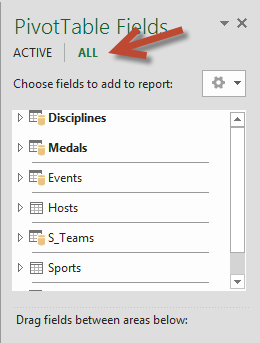
On Sheet1, at the top ofPivotTable Fields, clickAll to view the complete list of available tables, as shown in the following screen.
-
Scroll through the list to see the new tables you just added.
-
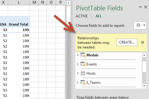
Expand Sports and select Sport to add it to the PivotTable. Notice that Excel prompts you to create a relationship, as seen in the following screen.
This notification occurs because you used fields from a table that’s not part of the underlying Data Model. One way to add a table to the Data Model is to create a relationship to a table that’s already in the Data Model. To create the relationship, one of the tables must have a column of unique, non-repeated, values. In the sample data, the Disciplines table imported from the database contains a field with sports codes, called SportID. Those same sports codes are present as a field in the Excel data we imported. Let’s create the relationship.
-
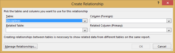
Click CREATE… in the highlighted PivotTable Fields area to open the Create Relationship dialog, as shown in the following screen.
-
In Table, choose Disciplines from the drop down list.
-
In Column (Foreign), choose SportID.
-
In Related Table, choose Sports.
-
In Related Column (Primary), choose SportID.
-
Click OK.
The PivotTable changes to reflect the new relationship. But the PivotTable doesn’t look right quite yet, because of the ordering of fields in the ROWS area. Discipline is a subcategory of a given sport, but since we arranged Discipline above Sport in the ROWS area, it’s not organized properly. The following screen shows this unwanted ordering.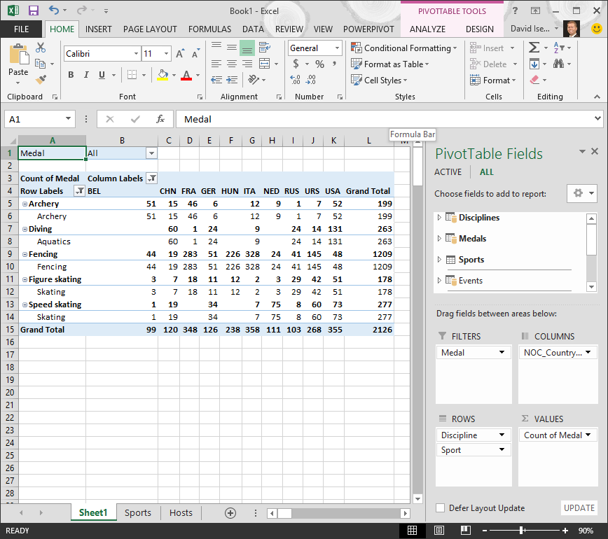
-
In the ROWS area, move Sport above Discipline. That’s much better, and the PivotTable displays the data how you want to see it, as shown in the following screen.
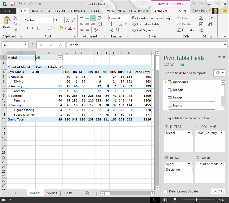
Behind the scenes, Excel is building a Data Model that can be used throughout the workbook, in any PivotTable, PivotChart, in Power Pivot, or any Power View report. Table relationships are the basis of a Data Model, and what determine navigation and calculation paths.
In the next tutorial, Extend Data Model relationships using Excel 2013, Power Pivot, and DAX, you build on what you learned here, and step through extending the Data Model using a powerful and visual Excel add-in called Power Pivot. You also learn how to calculate columns in a table, and use that calculated column so that an otherwise unrelated table can be added to your Data Model.
Checkpoint and Quiz
Review What You’ve Learned
You now have an Excel workbook that includes a PivotTable accessing data in multiple tables, several of which you imported separately. You learned to import from a database, from another Excel workbook, and from copying data and pasting it into Excel.
To make the data work together, you had to create a table relationship that Excel used to correlate the rows. You also learned that having columns in one table that correlate to data in another table is essential for creating relationships, and for looking up related rows.
You’re ready for the next tutorial in this series. Here’s a link:
Extend Data Model relationships using Excel 2013, Power Pivot, and DAX
QUIZ
Want to see how well you remember what you learned? Here’s your chance. The following quiz highlights features, capabilities, or requirements you learned about in this tutorial. At the bottom of the page, you’ll find the answers. Good luck!
Question 1: Why is it important to convert imported data into tables?
A: You don’t have to convert them into tables, because all imported data is automatically turned into tables.
B: If you convert imported data into tables, they will be excluded from the Data Model. Only when they’re excluded from the Data Model are they available in PivotTables, Power Pivot, and Power View.
C: If you convert imported data into tables, they can be included in the Data Model, and be made available to PivotTables, Power Pivot, and Power View.
D: You cannot convert imported data into tables.
Question 2: Which of the following data sources can you import into Excel, and include in the Data Model?
A: Access Databases, and many other databases as well.
B: Existing Excel files.
C: Anything you can copy and paste into Excel and format as a table, including data tables in websites, documents, or anything else that can be pasted into Excel.
D: All of the above
Question 3: In a PivotTable, what happens when you reorder fields in the four PivotTable Fields areas?
A: Nothing – you cannot reorder fields once you place them in the PivotTable Fields areas.
B: The PivotTable format is changed to reflect the layout, but underlying data is unaffected.
C: The PivotTable format is changed to reflect the layout, and all underlying data is permanently changed.
D: The underlying data is changed, resulting in new data sets.
Question 4: When creating a relationship between tables, what is required?
A: Neither table can have any column that contains unique, non-repeated values.
B: One table must not be part of the Excel workbook.
C: The columns must not be converted to tables.
D: None of the above is correct.
Quiz Answers
-
Correct answer: C
-
Correct answer: D
-
Correct answer: B
-
Correct answer: D
Notes: Data and images in this tutorial series are based on the following:
-
Olympics Dataset from Guardian News & Media Ltd.
-
Flag images from CIA Factbook (cia.gov)
-
Population data from The World Bank (worldbank.org)
-
Olympic Sport Pictograms by Thadius856 and Parutakupiu
To create a data set using a Microsoft Excel file stored locally:
- Click the New Data Set toolbar button and select Microsoft Excel File.
- Enter a name for this data set.
- Select Local to enable the upload button.
- Click the Upload icon to browse for and upload the Microsoft Excel file from a local directory.
Contents
- 1 How do you create a dataset?
- 2 What is the dataset in Excel?
- 3 Can we create our own dataset?
- 4 Can I create my own dataset for machine learning?
- 5 How do I create an autofill form in Excel?
- 6 How do I create a data model in Excel?
- 7 What is a data set example?
- 8 How do you create a deep learning dataset?
- 9 How do you create a dataset of an image?
- 10 How do you prepare a dataset for analysis?
- 11 What is the process of creating and using a dataset?
- 12 How do you create a training dataset for machine learning?
- 13 What makes a good dataset?
- 14 How do I AutoFill an entire column in Excel?
- 15 How do I align two data sets in Excel?
- 16 How do you add data to a table?
- 17 What does a dataset look like?
- 18 What are dataset entries?
- 19 What are the types of data sets?
- 20 What is dataset in deep learning?
On the Create dataset page:
- For Dataset ID, enter a unique dataset name.
- For Data location, choose a geographic location for the dataset. After a dataset is created, the location can’t be changed.
- For Default table expiration, choose one of the following options:
- Click Create dataset.
What is the dataset in Excel?
A dataset is a range of contiguous cells on an Excel worksheet containing data to analyze. When arranging data on an Excel worksheet you must follow a few simple rules so that Analyse-it works with your data: Title to clearly describe the data.
Can we create our own dataset?
While you can get robust datasets from Kaggle, if you want to creating something fresh for you or your company, scraping is the way to go, for example. if you want to build a price recommendation for shoes you would want the latest trends and prices from Amazon and not 2 years old data.
Can I create my own dataset for machine learning?
Dataset preparation is sometimes a DIY project
If you were to consider a spherical machine-learning cow, all data preparation should be done by a dedicated data scientist.So, let’s have a look at the most common dataset problems and the ways to solve them.
How do I create an autofill form in Excel?
Fill data automatically in worksheet cells
- Select one or more cells you want to use as a basis for filling additional cells. For a series like 1, 2, 3, 4, 5…, type 1 and 2 in the first two cells.
- Drag the fill handle .
- If needed, click Auto Fill Options. and choose the option you want.
How do I create a data model in Excel?
It can be any range of data, but data formatted as an Excel table is best. Use one of these approaches to add your data: Click Power Pivot > Add to Data Model. Click Insert > PivotTable, and then check Add this data to the Data Model in the Create PivotTable dialog box.
What is a data set example?
A data set is a collection of numbers or values that relate to a particular subject. For example, the test scores of each student in a particular class is a data set. The number of fish eaten by each dolphin at an aquarium is a data set.
How do you create a deep learning dataset?
Steps for Preparing Good Training Datasets
- Identify Your Goal. The initial step is to pinpoint the set of objectives that you want to achieve through a machine learning application.
- Select Suitable Algorithms. different algorithms are suitable for training artificial neural networks.
- Develop Your Dataset.
How do you create a dataset of an image?
Procedure
- From the cluster management console, select Workload > Spark > Deep Learning.
- Select the Datasets tab.
- Click New.
- Create a dataset from Images for Object Classification.
- Provide a dataset name.
- Specify a Spark instance group.
- Specify image storage format, either LMDB for Caffe or TFRecords for TensorFlow.
How do you prepare a dataset for analysis?
Data Preparation Steps in Detail
- Access the data.
- Ingest (or fetch) the data.
- Cleanse the data.
- Format the data.
- Combine the data.
- And finally, analyze the data.
What is the process of creating and using a dataset?
The process of creating a dataset involves three important steps:
- Data Acquisition.
- Data Cleaning.
- Data Labeling.
How do you create a training dataset for machine learning?
How to create a machine learning dataset from scratch?
- Detect individual letters in an image.
- Create a training dataset from these letters.
- Train an algorithm to classify the letters.
- Use the trained algorithm to classify individual letters (online)
What makes a good dataset?
A “good dataset” is a dataset that : Does not contains missing values. Does not contains aberrant data. Is easy to manipulate (logical structure).
How do I AutoFill an entire column in Excel?
Simply do the following:
- Select the cell with the formula and the adjacent cells you want to fill.
- Click Home > Fill, and choose either Down, Right, Up, or Left. Keyboard shortcut: You can also press Ctrl+D to fill the formula down in a column, or Ctrl+R to fill the formula to the right in a row.
How do I align two data sets in Excel?
Now you can create a new sheet and click on cell A1 in the new sheet. Now go to Data > Consolidate. In the popup select the range from your first sheet to the reference box and click on Add, after adding the first data select the reference box again and clear the reference box and add the second data set.
How do you add data to a table?
Add a row or column to a table by typing in a cell just below the last row or to the right of the last column, by pasting data into a cell, or by inserting rows or columns between existing rows or columns. To add a row at the bottom of the table, start typing in a cell below the last table row.
What does a dataset look like?
A dataset (example set) is a collection of data with a defined structure. Table 2.1 shows a dataset. It has a well-defined structure with 10 rows and 3 columns along with the column headers. This structure is also sometimes referred to as a “data frame”.
What are dataset entries?
ENTRY: Uses the Numeric data type and stores a value representing the order in which the entries are logged. The example includes seven separate entries by four people, and every entry has a unique number. ID: Uses the Numeric data type and stores an identifying number for the person associated with each entry.
What are the types of data sets?
Types of Data Sets
- Numerical data sets.
- Bivariate data sets.
- Multivariate data sets.
- Categorical data sets.
- Correlation data sets.
What is dataset in deep learning?
A data set is a collection of data.In Machine Learning projects, we need a training data set. It is the actual data set used to train the model for performing various actions.
Do you need to create and use a database? This post is going to show you how to make a database in Microsoft Excel.
Excel is the most common data tool used in businesses and personal productivity across the world.
Since Excel is so widely used and available, it tends to get used frequently to store and manage data as a makeshift database. This is especially true with small businesses since there is no budget or expertise available for more suitable tools.
This post will show you what a database is and the best practices you should follow if you’re going to try and use Excel as a database.

Get the example files used in this post with the above link and follow along below!
What is a Database?
A database is a structured set of data that is often in an electronic format and is used to organize, store. and retrieve data.
For example, a database might be used to store customer names, addresses, orders, and product information.
Databases often have key features that make them an ideal place to store your data.
Database vs Excel
An Excel spreadsheet is not a database, but it does have a lot of great and easy-to-use features for working with data.
Here are some of the key features of a database and how they compare to an Excel file.
| Feature | Database | Excel |
|---|---|---|
| Create, read, update, and delete records | ✔️ | ✔️ Excel allows anyone to add or edit data. This can be viewed as a negative consideration. |
| Data types | ✔️ | ⚠️ Excel allows for simple data types such as text, numbers, dates, boolean, images, and error values. But lacks more complex data types such as date and timezones, files, or JSON. |
| Data validation | ✔️ | ⚠️ Excel has some data validation features, but you can only apply one rule at a time and these can easily be overridden on purpose or by accident. |
| Access and security | ✔️ | ❌ Excel doesn’t have any access or security controls. This is usually managed through your on-premise network or through SharePoint online. But anyone can access your Excel file if it’s downloaded and sent to them. |
| Version control | ✔️ | ❌ Excel has no version control. This can be managed through SharePoint. |
| Backups | ✔️ | ❌ Excel has no automated backups. These can be manually created or automated in SharePoint. |
| Extract and query data | ✔️ | ✔️ Excel allows you to extract and query data through Power Query which is easy to learn and use. |
| Perform calculations | ✔️ | ✔️ Excel has a large library of functions that can be used in calculated columns inside tables. Excel also has the DAX formula language for calculated columns in Power Pivot. |
| Aggregate and summarize data | ✔️ | ✔️ Excel can easily aggregate and summarize data with formulas, pivot tables, or power pivots. |
| Relationships | ✔️ | ✔️ Excel has many lookup functions such as XLOOKUP, as well as table merge functionality in Power Query, and 1 to many relationships in Power Pivot. |
| Scale with large amounts of data | ✔️ | ⚠️ Excel can hold up to 1,048,576 rows of data in a single sheet. Tools like Power Query and Power Pivot can help you deal with larger amounts of data but they will be constrained based on your hardware specifications. |
| User friendly | ❌ A database might not be user-friendly and may come with a steep learning curve that your intended users won’t be able to handle. | ✔️ Most people have some experience with using Excel. |
| Cost | ❌ Can be expensive to set up, run, and maintain a proper database tool. | ✔️ Your organization might already have access to and use Excel. |
This is not a comprehensive list of features that a database will have, but they are some of the major features that will usually make a proper database a more suitable option.
The features that a database has depends on what database it is. Not all databases have the same features and functionality.
You will need to decide what features are essential for your situation in order to decide if you should use Excel or some other database tool.
💡 Tip: If you have Excel for Microsoft 365, then consider using Dataverse for Teams as your database instead of Excel. Dataverse has many of the great database features mentioned above and it is included in your Microsoft 365 license at no additional cost.
Relational Database Design
A good deal of thought should happen about the structure of your database before you begin to build it. This can save you a lot of headaches later on.
Most databases have a relational design. This means the database contains many related tables instead of one table that contains all the data.
Suppose you want to track orders in your database.
One option is to create a single flat table that contains all the information about the order, the products, and the customer that created the order.
This isn’t very efficient as you end up creating multiple entries of the same customer information such as name, email, and address. You can see in the above data, column G, H, and I contains a lot of duplicate values.
A better option is to create separate tables to store the Order, Product, and Customer data.
The Order data can then reference a unique identifier in the Product and Customer data that will relate the tables and avoid unnecessary duplicate data entry.
This same example data might look like this when reorganized into multiple related tables.
- An Orders table that contains the Item and Customer ID field.
- A Products table that relates to the Item fields in the Orders table.
- A Customers table that relates to the Customer ID in the Orders table.
This avoids duplicated data entry in a flat single table structure and you can use the Item or Customer ID unique identifier to look up the related data in the respective Products or Customers tables.
Tabular Data Structure in Excel
If you’re going to use Excel as your database, then you’re going to need your data in tabular format. This refers to the way the data is structured.
The above example shows a product order dataset in tabular format. A tabular data format is best suited for Excel due to the row and column structure of a spreadsheet.
Here are a few rules your data should follow so that it’s in tabular format.
- 1st row should contain column headings. This is just a short and descriptive name for the data contained below.
- No blank column headings. Every column of data should have a name.
- No blank columns or blank rows. Blank values within a field are ok, but columns or rows that are entirely blank should be removed.
- No subtotals or grand totals within the data.
- One row should represent exactly one record of data.
- One column should contain exactly one type of data.
In the above orders example data, you can see B2:E2 contains the column headings of an Order ID, Customer ID, Order Date, Item, and Quantity.
The dataset has no blank rows or columns, and no subtotals are included.
Each row in the dataset represents an order for one type of product.
You’ll also notice each column contains one type of data. For example, the Item column only contains information on the name of the product and does not include other product information such as the price.
⚠️ Warning: If you don’t adhere to this type of structure for your data, then summarizing and analyzing your data will be more difficult later. Tools such as pivot tables require tabular data!
Use Excel Tables to Store Data
Excel has a feature that is specifically for storing your tabular data.
An Excel Table is a container for your tabular datasets. They help keep all the same data together in one object with many other benefits.
💡 Tip: Check out this post to learn more about all the amazing features of Excel Tables.
You will definitely want to use a table to store and organize any data table that will be a part of your dataset.
How to Create an Excel Table
Follow these steps to create a table from an existing set of data.
- Select any cell inside your dataset.
- Go to the Insert tab in the ribbon.
- Select the Table command.
This will open the Create Table menu where you will be able to select the range containing your data.
When you select a cell inside your data before using the Table command, Excel will guess the full range of your dataset.
You will see a green dash line surrounding your data which indicates the range selected in the Create Table menu. You can click on the selector button to the right of the range input to adjust this range if needed.
- Check the My table has headers option.
- Press the OK button.
📝 Note: The My table has headers option needs to be checked if the first row in your dataset contains column headings. Otherwise, Excel will create a table with generic column heading titles.
Your Excel data will now be inside a table! You will immediately see that it’s inside a table as Excel will apply some default format which will make the table range very obvious.
💡 Tip: You can choose from a variety of format options for your table from the Table Design tab in the Table Styles section.
The next thing you will want to do with your table is to give it a sensible name. The table name will be used to reference the table in formulas and other tools, so giving it a short descriptive name will help you later when reading formulas.
- Go to the Table Design tab.
- Click on the Table Name input box.
- Type your new table name.
- Press the Enter key to accept the new name.
Each table in your database will need to be in a separate table, so you will need to repeat the above process for each.
How to Add New Data to Your Table
You will likely need to add new records to your database. This means you will need to add new rows to your tables.
Adding rows to an Excel table is very easy and you can do it a few different ways.
You can add new rows to your table from the right-click menu.
- Select a cell inside your table.
- Right-click on the cell.
- Select Insert from the menu.
- Select Table Rows Above from the submenu.
This will insert a new blank row directly above the selected cells in your table.
You can add a blank row to the bottom of your table with the Tab key.
- Place the active cell cursor in the lower right cell of the table.
- Press the Tab key.
A new blank row will be added to the bottom of the table.
But the easiest way to add new data to a table is to type directly below the table. Data entered directly underneath the table is automatically absorbed into the table!
Excel Workbook Layout
If you are going to create an Excel database, then you should keep it simple.
Your Excel database file should contain only the data and nothing else. This means any reports, analysis, data visualization, or other work related to the data should be done in another Excel file.
Your Excel database file should only be used for adding, editing, or deleting the data stored in the file. This will help decrease the chance of accidentally changing your data, as the only reason to open the file will be to intentionally change the data.
Each table in the database should be stored in a separate worksheet and nothing else except the table should be in that sheet. You can then name the worksheet based on the table it contains so your file is easy to navigate.
💡 Tip: Place your table starting in cell A1 and then hide the remaining columns. This way it is clear the sheet should only contain the table and nothing else.
The only other sheet you might optionally include is a table of contents to help organize the file. This is where you can list each table along with the fields it contains and a description of what these fields are.
💡 Tip: You can hyperlink the table name listed in the table of contents to its associated sheet. Select the name and press Ctrl + K to create a hyperlink. This can help you navigate the workbook when you have a lot of tables in your database.
Use Data Validation to Prevent Invalid Data
Data validation is a very important feature for any database. This allows you to ensure only specific types of data are allowed in a column.
You might create data validation rules such as.
- Only positive whole numbers are entered in a quantity column.
- Only certain product names are allowed in the product column.
- A column can’t contain any duplicate values.
- Dates are between two given dates.
Excel’s data validation tools will help you ensure the data entered in your database follow such rules.
Follow these steps to add a data validation rule to any column in your table.
- Left-click on the column heading to select the entire column.
When you hover the mouse cursor over the top of your column heading in a table, the cursor will change to a black downward pointing arrow. Left-click and the entire column will be selected.
The data validation will automatically propagate to any new rows added to the table.
- Go to the Data tab.
- Click on the Data Validation command.
This will open up the Data Validation menu where you will be able to choose from various validation settings. If there is no active validation in the cell, you should see the Any values option selected in the Allow criteria.
Only Allow Positive Whole Number Values
Follow these steps from the Data Validation menu to allow only positive whole number values to be entered.
- Go to the Settings tab in the Data Validation menu.
- Select the Whole number option from the Allow dropdown.
- Select the greater than option from the Data dropdown.
- Enter 0 in the Minimum input box.
- Press the OK button.
💡 Tip: Keep the Ignore blank option checked if you want to allow blank cells in the column.
This will apply the validation rule to the column and when a user tries to enter any number other than 1, 2, 3, etc… they will be warned the data is invalid.
Only Allow Items from a List
Selecting items from a dropdown list is a great way to avoid incorrect text input such as customer or product names.
Follow these steps from the Data Validation menu to create a dropdown list for selecting text values in a column.
- Go to the Settings tab in the Data Validation menu.
- Select the List option from the Allow dropdown.
- Check the In-cell dropdown option.
- Add the list of items to the Source input.
- Press the OK button.
📝 Note: If you place the list of possible options inside an Excel Table and select the full column for the Source reference, then the range reference will update as you add items to the table.
Now when you select a cell in the column you will see a dropdown list handle on the right of the cell. Click on this and you will be able to choose a value from a list.
Only Allow Unique Values
Suppose you want to ensure the list of products in your Products table is unique. You can use the Custom option in the validation settings to achieve this.
- Go to the Settings tab in the Data Validation menu.
- Select the Custom option from the Allow dropdown.
=(COUNTIFS(INDIRECT("Products[Item]"),A2)=1)- Enter the above formula in the Formula input.
- Press the OK button.
The formula counts the number of times the current row’s value appears in the Products[Item] column using the COUNTIFS function.
It then determines if this count is equal to 1. Only values where the formula evaluates to 1 are allowed which means the product name can’t have been in the list already.
📝 Note: You need to reference the column by name using the INDIRECT function in order for the range to grow as you add items to your table!
Show Input Message when Cell is Selected
The data validation menu allows you to show a message to your users when a cell is selected. This means you can add instructions about what types of values are allowed in the column.
Follow these steps to add an input message in the Data Validation menu.
- Go to the Input Message tab in the Data Validation menu.
- Keep the Show input message when cell is selected option checked.
- Add some text to the Title section.
- Add some text to the Input message section.
- Press the OK button.
When you select a cell in the column which contains the data validation, a small yellow pop-up will appear with your Title and Input message text.
Prevent Invalid Data with Error Message
When you have a data validation rule in place, you will usually want to prevent invalid data from being entered.
This can be achieved using the error message feature in the Data Validation menu.
- Go to the Error Alert tab in the Data Validation menu.
- Keep the Show error alert after invalid data is entered option checked.
- Select the Stop option in the Style dropdown.
- Add some text to the Title section.
- Add some text to the Error message section.
- Press the OK button.
📝 Note: The Stop option is essential if you want to prevent the invalid data from being entered rather than only warning the user the data is invalid.
When you try to enter a repeated value in the column your custom error message will pop up and prevent the value from being entered in the cell.
Data Entry Form for Your Excel Database
Excel doesn’t have any fool-proof methods to ensure data is entered correctly, even when data validation techniques previously mentioned are used.
When a user copies and pastes or cuts and pastes values, this can override data validation in a column and cause incorrect data to enter into your database.
Using a data entry form can help to avoid data entry errors and there are a couple of different options available.
- Use a table for data entry.
- Use the quick access toolbar data entry form.
- Use Microsoft Forms for data entry.
- Use Microsoft Power Automate app for data entry.
- Use Microsoft Power Apps for data entry.
💡 Tip: Check out this post for more details on the various data entry form options for Excel.
Tools such as Microsoft Forms, Power Automate, and Power Apps will give you more data validation, access, and security controls over your data entry compared with the basic Excel options.
Access and Security for Your Excel Database
Excel isn’t a secure option for your data.
Whatever measures you set up in your Excel file to prevent users from changing data by accident or on purpose will not be foolproof.
Whoever has access to the file will be able to create, read, update, and delete data from your database if they are determined. There are also no options to assign certain privileges to certain users within an Excel file.
However, you can manage access and security to the file from SharePoint.
💡 Tip: Check out this post from Microsoft about recommendations for securing SharePoint files for more details.
When you store your Excel file in SharePoint you’ll also be able to see recent changes.
- Go to the Review tab.
- Click on the Show Changes command.
This will open up the Changes pane on the right-hand side of the Excel sheet.
It will show you a chronological list of all the recent changes in the workbook, who made those changes, when they made the change, and what the previous value was.
You can also right-click on a cell and select Show Changes. This will open the Changes pane filtered to only show the changes for that particular cell.
This is a great way to track down the cause of any potential errors in your data.
Query Your Excel Database with Power Query
Your Excel database file should only be used to add, edit, or delete records in your tables.
So how do you use the data for anything else such as creating reports, analysis, or dashboards?
This is the magic of Power Query! It will allow you to connect to your Excel database and query the data in a read-only manner. You can build all your reports, analysis, and dashboards in a separate file which can easily be refreshed with the latest data from your Excel database file.
Here’s how to use power query to quickly import your data into any Excel file.
- Go to the Data tab.
- Click on the Get Data command.
- Choose the From File option.
- Choose the From Excel Workbook option in the submenu.
This will open a file picker menu where you can navigate to your Excel database file.
- Select your Excel database file.
- Click on the Import button.
⚠️ Warning: Make sure your Excel database file is closed or the import process will show a warning that it’s unable to connect to the file because it’s in use!
Clicking on the Import button will then open the Navigator menu. This is where you can select what data to load and where to load it.
The Navigator menu will list all the tables and sheets in the Excel file. Your tables might be listed with a suffix on the name if you’ve named the sheets and tables the same.
- Check the option to Select multiple items if you want to load more than one table from your database.
- Select which tables to load.
- Click on the small arrow icon next to the Load button.
- Select the Load To option in the Load submenu.
This will open the Import Data menu where you can choose to import your data into a Table, PivotTable, PivotChart, or only create a Connection to the data without loading it.
- Select the Table option.
- Click on the OK button.
Your data is then loaded into an Excel Table in the new workbook.
The best part is you can always get the latest data from the source database file. Go to the Data tab and press the Refresh All button to refresh the power query connection and import the latest data.
💡 Tip: You can do a lot more than just load data with Power Query. You can also transform your data in just about any imaginable way using the Transform Data button in the Navigator menu. Check out this post on how to use Power Query for more details about this amazing tool.
Analyze and Summarize Your Excel Database with Power Pivot
Power Query isn’t the only database tool Excel has. The data model and Power Pivot add-in will help you slice and dice relational data inside your Excel pivot tables.
When you load your data with Power Quer, there is an option to Add this data to the Data Model in the Import Data menu.
This option will allow you to build relationships between the various tables in your database. This way you’ll be able to analyze your orders by category even though this field doesn’t appear in the Orders table.
You can build your table relationships from the Data tab.
- Go to the Data tab.
- Click on either the Relationships or Manage Data Model command.
Now you’ll be able to analyze multiple tables from your database inside a single pivot table!
Conclusions
Data is an essential part of any business or organization. If you need to track customers, sales, inventory, or any other information then you need a database.
If you need to create a database on a budget with the tools you have available then Microsoft Excel might be the best option and is a natural fit for any tabular data because of its row and column structure.
There are many things to consider when using Excel as a database such as who will have access to the files, what type of data will be stored, and how you will use the data.
Features such as Tables, data validation, power query, and power pivot are all essential to properly storing, managing, and accessing your data.
Do you use Excel as a database? Do you have any other tips for using Excel to manage your dataset? Let me know in the comments below!
About the Author
John is a Microsoft MVP and qualified actuary with over 15 years of experience. He has worked in a variety of industries, including insurance, ad tech, and most recently Power Platform consulting. He is a keen problem solver and has a passion for using technology to make businesses more efficient.
Excel Create Database (Table of Contents)
- Create a Database in Excel
- How to Create a Database in Excel?
Introduction to Create Database in Excel
If you want to create a database, MS Access is the tool you ideally should look for. However, it is a bit complicated to learn and master the techniques therein as MS Access. It would help if you had ample time to master those. In such cases, you can use excel as a good resource to create a database. It is easier to enter, store, and find specific information in the Excel Database. A well-structured, well-formatted excel table can be considered as a database itself. So, all you have to do is create a table that has a proper format. If the table is well-structured, you can sort the data in many different ways. Moreover, you can apply the filters to well-structured data to slice and dice it as per your requirements.
How to Create a Database in Excel?
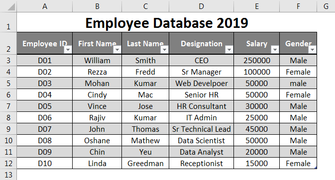
We’ll be creating an employee database for the organization. Let’s see how to create a database in Excel by following the below process:
You can download this Create Database Excel Template here – Create Database Excel Template
Data Entering to Create Excel Database
Data entering is the main aspect while you are trying to create a database in Excel.
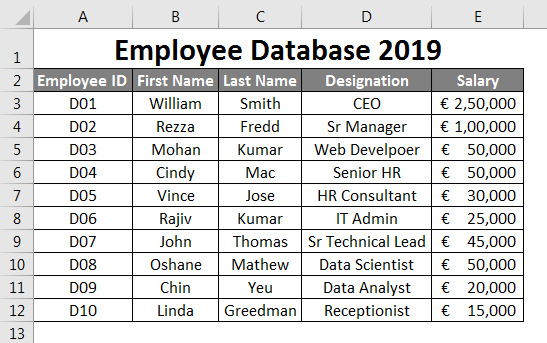
Suppose this is the data thatq1 you are going to use as an employee database.
I have added the first few Employee ID’s. Say D01, D02, D03 and then dragged the remaining till row 12 using Fill Handle. Column second onwards contains the general employee information like First Name, Last Name, Designation, and Salary. Filthis informationon in cells manually as per your details. Make sure the Salary column format is applied to all the cells in the column (Otherwise, this database may cause an error while using).
Entering Correct Data
It is always good to enter the correct data. Make sure there is no space in your data. When I say no other blanks, it covers the column cells, which are not blank as well. Try to the utmost that no data cells are blank. If you don’t have any information available with you, prefer to put NA over a blank cell. It’s also important to make the right input to the right column.
See the screenshot below:
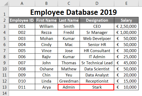
Suppose,uy as shown in the image above, you wrongly interchanged the column inputs. i.e. you have mentioned Designation under Last Name and Last Name under Designation, which is a serious drop-back when you are thinking of this as a master employee data for your organization. It may mislead some of your conclusions.
Suppose you have added a correct entry, but at the 2nd row after the last row (i.e. one row is left blank). It is also not recommended to do so. It is a breakdown for your data. See screenshot given below:
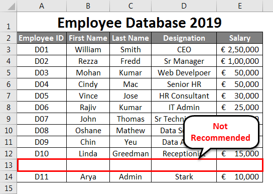
As you can see, there is one row left blank after row no. 12 ( second last row of the dataset) and added one new row, which is not recommended. On similar lines, you should not leave any blank column in the database.
Let’s see the screenshot below:
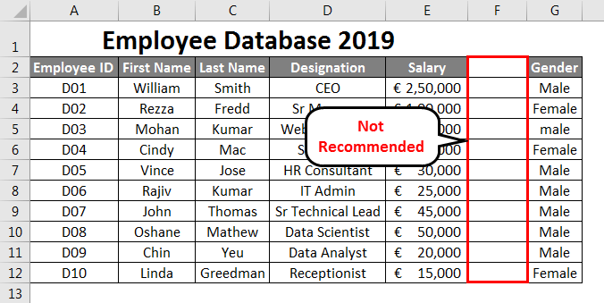
As you can see, column F is left blank. Which causes Excel to think there is a split of data. Excel considers that a blank column is a separator for two databases. It is misleading, as the column after the blank column is a part of your original database. It’s not the start column of a new database.
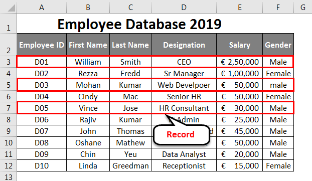
All the Rows are called Record in Excel Database.
It is a kind of basic knowledge we should have about the database we are creating. Every single row we create/add is called as a Record in the database. See the below screenshot for your reference:
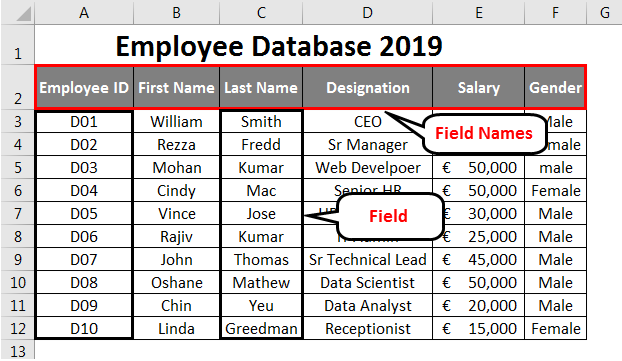
Every Column is a Field in Excel Database
Every column is called Field in the Excel database. The column headings are called Field Names.
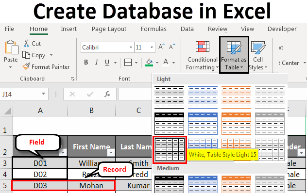
Format Table
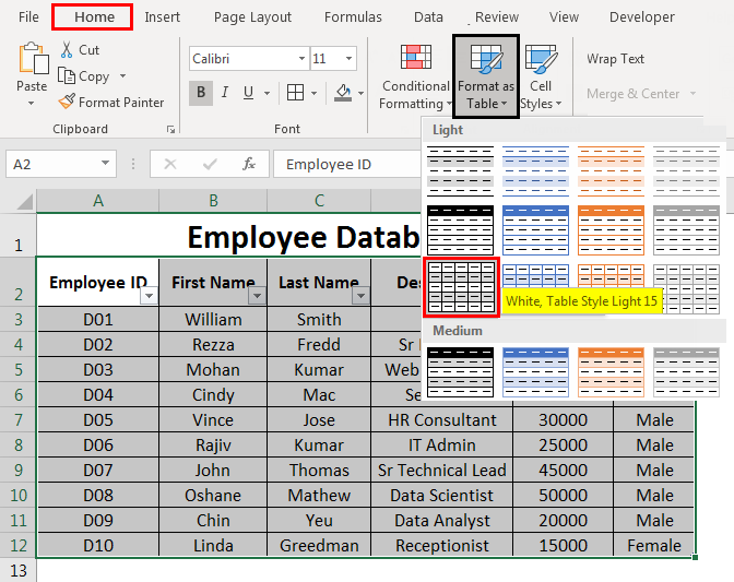
Once you are done with inputting the data, it should be converted into a better visualisation table.
- Select cells A2 to F12 from the spreadsheet.
- Go to the Home tab.
- Select Format as Table drop-down menu. You can choose a table layout of your own.
Once you click a particular table format, a table window will pop up with the range of data selected, and a dotted line will surround that range. You can change the range of the data therein in the table dialog box as well.
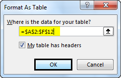
Once you are happy with the range, you can choose, OK. You can see your data in a tabular form now. See the screenshot given below:
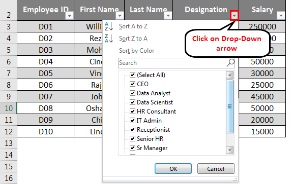
Use Excel Database Tools to Sort or Filter the Data
You can use the drop-down arrows situated beside each Field Name to Sort or Filter the data as per your requirement. These options are really helpful when you are dealing with a large amount of data.
Expanding the Database
If you want to add some more records to your table, you can do it as well. Select all the cells from your table.
Place your mouse at the bottom of the last cell of your table. The mouse pointer will turn into a two-headed arrow. You can drag down the pointer from there until you want to add that many blank rows in your database. Subsequently, you can add data under those blank cells as well.
Database Formatting
Highlight cell A1 to F1 from the spreadsheet.
- Select Home tab
- Under the Home tab, go to Wrap Text as well as Merge and Center.
- You can also change the fill colour. Select Fill Color. Choose the colour of your interest. Here I have selected Green as a colour.
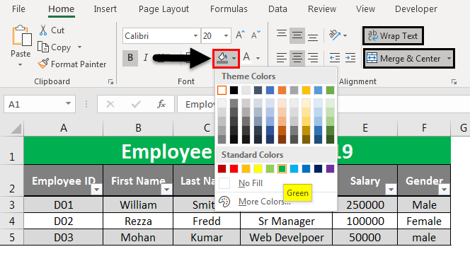
This is how we have created our Database in Excel.
Things to Remember About Create Database in Excel
- Information about one item should be populated in one single row entirely. You can’t use multiple lines to add different data of the same item in the excel database.
- The field should not be kept empty. (Including Column Headings/Field Name).
- The data type entered in one column should be homogeneous. For, e.g. If you are entering Salary details in the Salary column, there should not be any text string in that column. Similarly, any column containing text strings should not contain any numerical information.
- The database created here is really a very small example. It becomes huge in terms of employees joining every now and then and becomes hectic to maintain the data again and again with the standard formatting. That’s why it is recommended to use databases.
Recommended Articles
This has been a guide to Create a Database in Excel. Here we discuss how to Create a Database in Excel along with practical examples and a downloadable excel template. You can also go through our other suggested articles –
- Excel Import Data
- Table styles in Excel
- Toolbar in Excel
- Excel Rows and Columns