
Insert cells
- Right-click the cell above which you want to insert a new cell.
- Select Insert, and then select Cells & Shift Down.
Contents
- 1 How do I make a cell on Excel?
- 2 How do I add a cell between cells in Excel?
- 3 What is Cell of MS Excel?
- 4 How do you make Excel automatically add rows?
- 5 How do you insert a cell?
- 6 How do I paste multiple cells into one cell?
- 7 How do you insert a cell in Excel using the keyboard?
- 8 How do I put text in the middle of a cell in Excel?
- 9 Where is cell in Excel?
- 10 How is cell formed in computer?
- 11 How do I add a column to a table in Excel?
- 12 How do I automatically copy cells in Excel?
- 13 How do I create a formula for multiple cells in Excel?
- 14 How do you insert cells in Excel without changing formulas?
- 15 How do you copy multiple cells in Excel into one cell?
- 16 How do you combine cells in Excel without losing data?
- 17 How do I copy and paste a list into one cell in Excel?
- 18 How do I insert a cell in Excel without a mouse?
- 19 How do I open a cell in Excel?
- 20 What does Ctrl Shift do in Excel?
How do I make a cell on Excel?
To add a new individual cell to an Excel spreadsheet, follow the steps below.
- Select the cell of where you want to insert a new cell by clicking the cell once with the mouse.
- Right-click the cell of where you want to insert a new cell.
- In the right-click menu that appears, select Insert.
How do I add a cell between cells in Excel?
To insert cells:
- Select the location where the new cell(s) will be inserted.
- Right-click and choose Insert.
- The Insert dialog box opens.
- Shift cells right to shift cells in the same row to the right.
- Shift cells down to shift selected cells and all cells in the column below it downward.
- Choose an option, then click OK.
What is Cell of MS Excel?
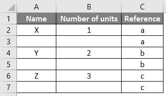
Cells are the boxes you see in the grid of an Excel worksheet, like this one. Each cell is identified on a worksheet by its reference, the column letter and row number that intersect at the cell’s location. This cell is in column D and row 5, so it is cell D5. The column always comes first in a cell reference.
How do you make Excel automatically add rows?
Select the entire row which you want to insert a blank row above, and press Shift + Ctrl + + keys together, then a blank row is inserted.
How do you insert a cell?
Insert cells
- Right-click the cell above which you want to insert a new cell.
- Select Insert, and then select Cells & Shift Down.
How do I paste multiple cells into one cell?
If you want to paste all the contents into one cell, you can use this method.
- Press the shortcut key “Ctrl + C” on the keyboard.
- And then switch to the Excel worksheet.
- Now double click the target cell in the worksheet.
- After that, press the shortcut key “Ctrl + V” on the keyboard.
How do you insert a cell in Excel using the keyboard?
Your options are:
- Ctrl + Shift + “+” + I: Shifts cells right to insert cell.
- Ctrl + Shift + “+” + D: Shift cells down to insert cell.
- Ctrl + Shift + “+” + R: Inserts entire row.
- Ctrl + Shift + “+” + C: Inserts entire column.
How do I put text in the middle of a cell in Excel?
Align text in a cell
- Select the cells that have the text you want aligned.
- On the Home tab choose one of the following alignment options:
- To vertically align text, pick Top Align , Middle Align , or Bottom Align .
- To horizontally align text, pick Align Text Left , Center , or Align Text Right .
Where is cell in Excel?
In Microsoft Excel, a cell is a rectangular box that occurs at the intersection of a vertical column and a horizontal row in a worksheet.
How is cell formed in computer?
A cell is an area on a spreadsheet where data can be entered.Cells are boxes formed by the intersection of vertical and horizontal lines that divide the spreadsheet into columns and rows.
How do I add a column to a table in Excel?
To insert a column, pick any cell in the table and right-click. Point to Insert, and pick Table Rows Above to insert a new row, or Table Columns to the Left to insert a new column.
How do I automatically copy cells in Excel?
Copy Values from Above
- In the first selected blank cell (such as A3) enter an equal sign and point to the cell above. As the cell is already selected, you don’t have to actually click A3.
- Press [Ctrl] + [Enter] and Excel will copy the respective formula to all blank cells in the selected range.
How do I create a formula for multiple cells in Excel?
Just select all the cells at the same time, then enter the formula normally as you would for the first cell. Then, when you’re done, instead of pressing Enter, press Control + Enter. Excel will add the same formula to all cells in the selection, adjusting references as needed.
How do you insert cells in Excel without changing formulas?
Select the formula in the cell using the mouse, and press Ctrl + C to copy it. Select the destination cell, and press Ctl+V. This will paste the formula exactly, without changing the cell references, because the formula was copied as text.
How do you copy multiple cells in Excel into one cell?
Move multiple cells into one with Clipboard
- Enable the Clipboard pane with clicking the anchor at the bottom-right corner of Clipboard group on the Home tab.
- Select the range of cells you will move to a single cell, and copy it with pressing the Ctrl + C keys in a meanwhile.
How do you combine cells in Excel without losing data?
How to merge cells in Excel without losing data
- Select all the cells you want to combine.
- Make the column wide enough to fit the contents of all cells.
- On the Home tab, in the Editing group, click Fill > Justify.
- Click Merge and Center or Merge Cells, depending on whether you want the merged text to be centered or not.
How do I copy and paste a list into one cell in Excel?
To paste a bullet list from Word into a single cell in Excel, copy the bullet list in Word, toggle to Excel, select the desired cell, press the F2 key to invoke edit mode, and then paste, as suggested by the screenshots below. The bullet list will paste into a single Excel cell.
How do I insert a cell in Excel without a mouse?
Keyboard shortcut to insert a row in Excel
- Shift+Spacebar to select the row.
- Alt+I+R to add a new row above.
How do I open a cell in Excel?
You can also press Ctrl+Shift+F or Ctrl+1. In the Format Cells popup, in the Protection tab, uncheck the Locked box and then click OK. This unlocks all the cells on the worksheet when you protect the worksheet.
What does Ctrl Shift do in Excel?
Press Ctrl + Shift + $ to apply Currency format, Ctrl + Shift + ~ to apply General number format, Ctrl + Shift % to apply Percentage format, Ctrl + Shift + # to apply Date format, Ctrl + Shift + @ to apply Time format, Ctrl + Shift + ! to apply Number format with two decimal places and thousands separator, and Ctrl +
Содержание
- CELL function
- Syntax
- info_type values
- CELL format codes
- How to create a table in Excel
- Excel table
- How to create a table in Excel
- How to make a table with a selected style
- How to name a table in Excel
- How to use tables in Excel
- How to filter a table in Excel
- How to sort a table in Excel
- Excel table formulas
- Sum table columns
- How to extend a table in Excel
- Excel table styles
- How to change table style
- Apply a table style and remove existing formatting
- Manage banded rows and columns
- How to remove table formatting
- How to remove table in Excel
CELL function
The CELL function returns information about the formatting, location, or contents of a cell. For example, if you want to verify that a cell contains a numeric value instead of text before you perform a calculation on it, you can use the following formula:
This formula calculates A1*2 only if cell A1 contains a numeric value, and returns 0 if A1 contains text or is blank.
Note: Formulas that use CELL have language-specific argument values and will return errors if calculated using a different language version of Excel. For example, if you create a formula containing CELL while using the Czech version of Excel, that formula will return an error if the workbook is opened using the French version. If it is important for others to open your workbook using different language versions of Excel, consider either using alternative functions or allowing others to save local copies in which they revise the CELL arguments to match their language.
Syntax
The CELL function syntax has the following arguments:
A text value that specifies what type of cell information you want to return. The following list shows the possible values of the Info_type argument and the corresponding results.
The cell that you want information about.
If omitted, the information specified in the info_type argument is returned for cell selected at the time of calculation. If the reference argument is a range of cells, the CELL function returns the information for active cell in the selected range.
Important: Although technically reference is optional, including it in your formula is encouraged, unless you understand the effect its absence has on your formula result and want that effect in place. Omitting the reference argument does not reliably produce information about a specific cell, for the following reasons:
In automatic calculation mode, when a cell is modified by a user the calculation may be triggered before or after the selection has progressed, depending on the platform you’re using for Excel. For example, Excel for Windows currently triggers calculation before selection changes, but Excel for the web triggers it afterward.
When Co-Authoring with another user who makes an edit, this function will report your active cell rather than the editor’s.
Any recalculation, for instance pressing F9, will cause the function to return a new result even though no cell edit has occurred.
info_type values
The following list describes the text values that can be used for the info_type argument. These values must be entered in the CELL function with quotes (» «).
Reference of the first cell in reference, as text.
Column number of the cell in reference.
The value 1 if the cell is formatted in color for negative values; otherwise returns 0 (zero).
Note: This value is not supported in Excel for the web, Excel Mobile, and Excel Starter.
Value of the upper-left cell in reference; not a formula.
Filename (including full path) of the file that contains reference, as text. Returns empty text («») if the worksheet that contains reference has not yet been saved.
Note: This value is not supported in Excel for the web, Excel Mobile, and Excel Starter.
Text value corresponding to the number format of the cell. The text values for the various formats are shown in the following table. Returns «-» at the end of the text value if the cell is formatted in color for negative values. Returns «()» at the end of the text value if the cell is formatted with parentheses for positive or all values.
Note: This value is not supported in Excel for the web, Excel Mobile, and Excel Starter.
The value 1 if the cell is formatted with parentheses for positive or all values; otherwise returns 0.
Note: This value is not supported in Excel for the web, Excel Mobile, and Excel Starter.
Text value corresponding to the «label prefix» of the cell. Returns single quotation mark (‘) if the cell contains left-aligned text, double quotation mark («) if the cell contains right-aligned text, caret (^) if the cell contains centered text, backslash () if the cell contains fill-aligned text, and empty text («») if the cell contains anything else.
Note: This value is not supported in Excel for the web, Excel Mobile, and Excel Starter.
The value 0 if the cell is not locked; otherwise returns 1 if the cell is locked.
Note: This value is not supported in Excel for the web, Excel Mobile, and Excel Starter.
Row number of the cell in reference.
Text value corresponding to the type of data in the cell. Returns «b» for blank if the cell is empty, «l» for label if the cell contains a text constant, and «v» for value if the cell contains anything else.
Returns an array with 2 items.
The 1st item in the array is the column width of the cell, rounded off to an integer. Each unit of column width is equal to the width of one character in the default font size.
The 2nd item in the array is a Boolean value, the value is TRUE if the column width is the default or FALSE if the width has been explicitly set by the user.
Note: This value is not supported in Excel for the web, Excel Mobile, and Excel Starter.
CELL format codes
The following list describes the text values that the CELL function returns when the Info_type argument is «format» and the reference argument is a cell that is formatted with a built-in number format.
Источник
How to create a table in Excel
 by Svetlana Cheusheva, updated on March 15, 2023
The tutorial explains the essentials of the table format, shows how to make a table in Excel and leverage its powerful features.
At the surface, an Excel table just sounds like a way to organize data. In truth, this generic name covers a ton of useful features. Tables containing hundreds or even thousands of rows and columns can be instantly recalculated and totaled, sorted and filtered, updated with new information and reformatted, summarized with pivot tables and exported.
Excel table
You might be under the impression that the data in your worksheet is already in a table simply because it’s organized in rows and columns. However, the data in a tabular format is not a true «table» unless you’ve specifically made it such.
Excel table is a special object that works as a whole and allows you to manage the table’s contents independently from the rest of the worksheet data.
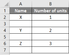
The screenshot below contrasts a regular range and the table format: 
The most obvious difference is that the table is styled. However, an Excel table is far more than a range of formatted data with headings. There are many powerful features inside:
- Excel tables are dynamic by nature, meaning they expand and contract automatically as you add or remove rows and columns.
- Integrated sort and filter options; visual filtering with slicers.
- Easy formatting with inbuilt table styles.
- Column headings remain visible while scrolling.
- Quicktotals allow you to sum and count data as well as find average, min or max value in a click.
- Calculated columns allow you to compute an entire column by entering a formula in one cell.
- Easy-to-read formulas due to a special syntax that uses table and column names rather than cell references.
- Dynamic charts adjust automatically as you add or remove data in a table.
How to create a table in Excel
With the source data organized in rows and columns, carry out the below steps to covert a range of cells into a table:
- Select any cell within your data set.
- On the Insert tab, in the Tables group, click the Table button or press the Ctrl + T shortcut.
- The Create Table dialog box appears with all the data selected for you automatically; you can adjust the range if needed. If you want the first row of data to become the table headers, make sure the My table has headers box is selected.
- Click OK.
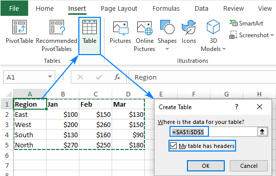
As the result, Excel converts your range of data into a true table with the default style: 
Many wonderful features are now just a click away and, in a moment, you will learn how to use them. But first, we’ll look at how to make a table with a specific style.
- Prepare and clean your data before creating a table: remove blank rows, give each column a unique meaningful name, and make sure each row contains information about one record.
- When a table is inserted, Excel retains all formatting that you currently have. For best results, you may want to remove some of the existing formatting, e.g. background colors, so it does not conflict with a table style.
- You are not limited to just one table per sheet, you can have as many as needed. For better readability, it stands to reason to insert at least one blank row and one blank column between a table and other data.
How to make a table with a selected style
The previous example showed the fastest way to create a table in Excel, but it always uses the default style. To draw a table with the style of your choosing, perform these steps:
- Select any cell in your data set.
- On the Home tab, in the Styles group, click Format as Table.
- In the gallery, click on the style you want to use.
- In the Create Table dialog box, adjust the range if necessary, check the My table has headers box, and click OK.
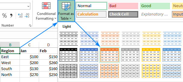
Tip. To apply the selected style and remove all existing formatting, right-click the style and choose Apply and Clear Formatting from the context menu.
How to name a table in Excel
Every time you make a table in Excel, it automatically gets a default name such asTable1, Table2, etc. When you deal with multiple tables, changing the default names to something more meaningful and descriptive can make your work a lot easier.
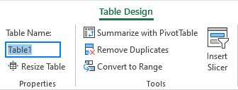
To rename a table, just do the following:
- Select any cell in the table.
- On the Table Design tab, in the Properties group, select the existing name in the Table Name box, and overwrite it with a new one.
Tip. To view the names of all tables in the current workbook, press Ctrl + F3 to open the Name Manager.
How to use tables in Excel
Excel tables have many awesome features that simply calculating, manipulating and updating data in your worksheets. Most of these features are intuitive and straightforward. Below you will find a quick overview of the most important ones.
How to filter a table in Excel
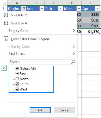
All tables get the auto-filter capabilities by default. To filter the table’s data, this is what you need to do:
- Click the drop-down arrow in the column header.
- Uncheck the boxes next to the data you want to filter out. Or uncheck the Select All box to deselect all the data, and then check the boxes next to the data you want to show.
- Optionally, you can use the Filter by Color and Text Filters options where appropriate.
- Click OK.
If you don’t need the auto-filter feature, you can remove the arrows by unchecking the Filter Button box on the Design tab, in the Table Style Options group. Or you can toggle the filter buttons on and off with the Ctrl + Shift + L shortcut. 
Additionally, you can create a visual filter for your table by adding a slicer. For this, click Insert Slicer on the Table Design tab, in the Tools group. 
How to sort a table in Excel
To sort a table by a specific column, just click the drop-down arrow in the heading cell, and pick the required sorting option: 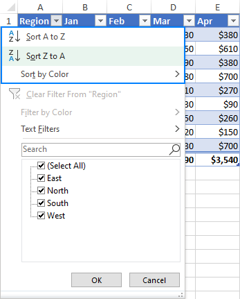
Excel table formulas
For calculating the table data, Excel uses a special formula syntax called structured references. Compared to regular formulas, they have a number of advantages:
- Easy-to-create. Simply select the table’s data when making a formula, and Excel will build a structured reference for you automatically.
- Easy-to-read. Structured references refer to the table parts by name, which makes formulas easier to understand.
- Auto-filled. To perform the same calculation in each row, enter a formula in any single cell, and it will be immediately copied throughout the column.
- Changed automatically. When you modify a formula anywhere in a column, the other formulas in the same column will change accordingly.
- Updated automatically. Every time the table is resized or the columns renamed, structured references update dynamically.
The screenshot below shows an example of a structured reference that sums data in each row: 
Sum table columns
Another great feature of an Excel table is the ability to summarize data without formulas. This option is called Total Row.
To sum a table’s data, this is what you need to do:
- Select any cell in the table.
- On the Design tab, in the Table Style Options group, put a tick mark in the Total Row box.
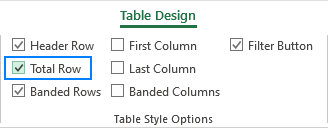
The Total row is inserted at the bottom of the table and shows the total in the last column: 
To sum data in other columns, click in the Total cell, then click the drop-down arrow and choose the SUM function. To calculate data in a different way, e.g. count or average, select the corresponding function.
Whatever operation you choose, Excel would use the SUBTOTAL function that calculates data only in visible rows: 
Tip. To toggle the Total Row on and off, use the Ctrl + Shift + T shortcut.
How to extend a table in Excel
When you type anything in an adjacent cell, an Excel table expands automatically to include the new data. Combined with structured references, this creates a dynamic range for your formulas without any effort from your side. If you don’t mean the new data to be part of the table, press Ctrl + Z . This will undo the table expansion but keep the data that you typed.
You can also extend a table manually by dragging a little handle at the bottom-right corner. 
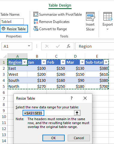
You can also add and remove columns and rows by using the Resize Table command. Here’s how:
- Click anywhere in your table.
- On the Design tab, in the Properties group, click Resize Table.
- When the dialog box appears, select the range to be included in the table.
- Click OK.
Excel table styles
Tables are very easily formatted due to a predefined gallery of styles. Additionally, you can create a custom style with your own formatting.
How to change table style
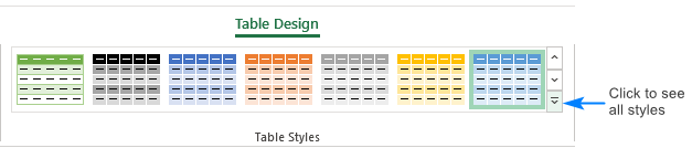
When you insert a table in Excel, the default style is automatically applied to it. To change a table style, do the following:
- Select any cell in the table.
- On the Design tab, in the Table Styles group, click on the style you want to apply. To see all the styles, click the More button in the down-right corner.
- To create your own style, please follow these guidelines: How to make a custom table style.
- To change the default table style, right-click the desired style and choose Set as Default. Any new table that you create in the same workbook will now be formatted with the new the default table style.
Apply a table style and remove existing formatting
When you format a table with any predefined style, Excel preserves the formatting you already have. To remove any existing formatting, right-click the style and choose Apply and Clear formatting: 
Manage banded rows and columns
To add or remove banded rows and columns as well as apply special formatting for the first or last column, simply tick or untick the corresponding checkbox on the Design tab in the Table Style Options group: 
How to remove table formatting
If you’d like to have all the functionality of an Excel table but do not want any formatting such as banded rows, table borders and the like, you can remove formatting in this way:
- Select any cell within your table.
- On the Design tab, in the Table Styles group, click the More button in the bottom-right corner, and then click Clear underneath the table style templates. Or pick the first style under Light, which is called None.

Note. This method only removes the inbuilt table formatting, your custom formatting is preserved. To remove absolutely all formatting in a table, go to the Home tab > Formats group, and click Clear > Clear formats.
How to remove table in Excel
Removing a table is as easy as inserting it. To convert a table back to a range, just do the following:
- Right-click any cell in your table, and then click Table>Convert to Range. Or click the Convert to Range button on the Design tab, in the Tools group.
- In the dialog box that appear, click Yes.
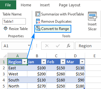
This will remove the table but retain all the data and formatting. To keep only the data, remove table formatting before converting your table to a range.
This is how you create, edit and remove a table in Excel. I thank you for reading and hope to see you on our blog next week!
Источник
Inserting rows and columns in Excel is very convenient when formatting tables and sheets. But function of inserting cells and entire adjacent and non-adjacent ranges enhances program features to new level.
Consider the practical examples how to add (or remove) cells and their ranges in the spreadsheet in Excel. In fact the cells are not added as the value moves on other. This fact should be taken into account when the sheet is filled with more than 50%. Then the remaining amount of cells for rows or columns may not be enough and this operation will delete the data. In such cases you should divide content of one sheet into 2 or 3 sheets. This is one of the main reasons why the new Excel version has more numbers of columns and rows (65,000 lines in the older versions and 1 000 000 in new one).
Inserting a range of empty cells
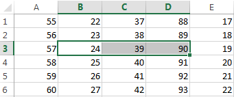
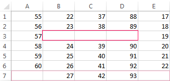
How to insert a cell in an Excel spreadsheet? Let’s say we have a table of values to which you want to insert two empty cells in between.
Perform the following procedure:
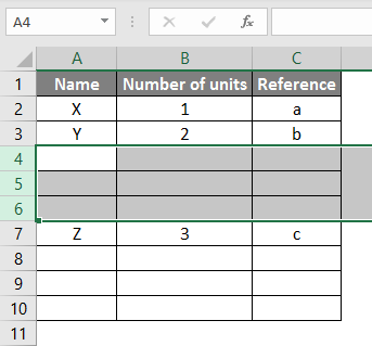
- Select the range in the place where you need to add new empty blocks. Go to the tab «HOME» — «Insert» — «Insert Cells». Or simply right click on the highlighted area and select the paste option. Or you may press the hotkey combination CTRL + SHIFT + «+».
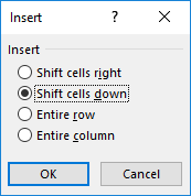
- A «Insert» dialog box appears where it is necessary to set the required parameters. In this case select «Shift down».
- Click OK. After that in the table with values new cells will be added. And the old will retain values and move down giving its place.
In this situation you can simply press the tool «HOME» — «Insert» (without choosing other options). Then the new cells will be inserted and the old ones will shift down (by default) without calling the dialog box options.
Use hotkeys combination CTRL + SHIFT + «plus» to add cells in Excel after selecting them.
Note. Pay attention to the settings dialog box. The last two parameters allow us to insert rows and columns in the same manner.
Removing cells
Now let’s remove the same range from our table with values. Just select the desired range. Right-click on the selected range and choose «Delete». Or go to the tab «HOME» — «Delete», «Shift up». The result is inversely proportional to the previous result.
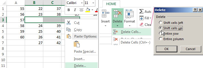
Select the range and use shortcut keys CTRL + «negative» if you want to remove cells in Excel.
Note. Likewise you can delete rows and columns.
Attention! In practice using tools «Insert» or «Delete» while inserting or deleting ranges without window with settings should be avoided so as not to get lost in the large and complex tables. Use the hotkeys if you want to save time. They cause a dialog box with removing the paste options and it also allows you to cope with the task much quickly.
How to Add Cells in Excel (Table of Contents)
- Adding Cells in Excel
- Examples of Add Cells in Excel
Adding Cells in Excel
Adding a cell is nothing but inserting a new cell or group of cells in between the existing cells by using the insert option in excel. We can insert the cells in row-wise or column-wise as per requirement, which allows us to input the additional data or new data in between the existing data.
Explanation: Sometimes, while working with Excel, we may forget to add some portion of date that should be inserted in between the existing data. In that case, we can cut the data and paste it a bit down or right and can input the required data in the gap. However, we can achieve the same without using the cut and paste option but by using the insert option in Excel.
There are four different options available to insert new cells. We will see each option and the respective example.
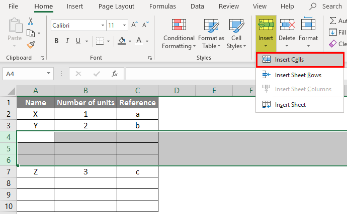
We can insert new cells in two ways; one way is to select the insert option from the worksheet, and the other is the shortcut key. Click on the “Home” menu at the top left corner in case if you are in a different menu.
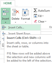
After the selection of “Home”, observe the right-hand side we have a section called “cells”. Which covers the options like “Insert”, “Delete”, and “format”, which are highlighted with a red colour box.
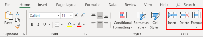
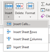
Each option has a drop-down if we observe under each option name. Click on the Insert option drop down then the drop-down menu will appear as below.
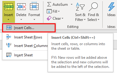
It has four different options: insert cells, insert sheet rows, insert sheet columns, and insert sheet. Click on the option Insert cells; then it will open a pop-up menu with four options as below.
Examples of Add Cells in Excel
Here are some examples of How to Add Cells in Excel, which are given below
You can download this How to Add Cells Excel Template here – How to Add Cells Excel Template
Example #1 – Add a Cell using Shift Cells Right
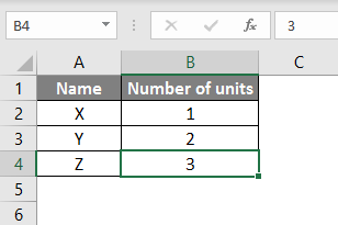
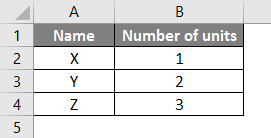
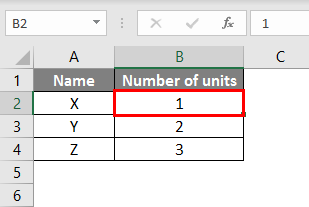
Consider a table having data of two columns like below.

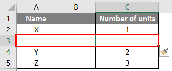
Now it has three rows of data. But in case if we need to add a cell at the cell B4 by moving the data to the right, we can do that. Follow the steps.
Step 1: Select the cell where you want to add a new cell. Here we have selected B4 as shown below.
Step 2: Select the Insert menu option for the drop-down as below.
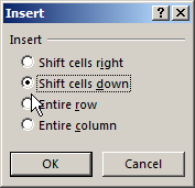
Step 3: Select the Insert Cells option then a pop-up menu will appear as below.
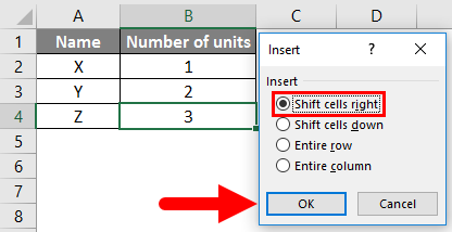
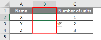
Step 4: Select the “Shift cells right” option, then click on OK. Then the result will appear as below.
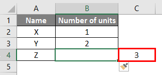
If we observe the above screen, number 3 is shifted to the right and created a new empty cell. This is how “shift cell right” will work. Similarly, we can do the shift cells down also.
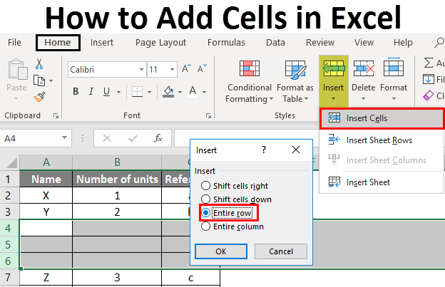
Example #2 – Insert a New Column and New Row
To add a new column, follow the below steps. It is as similar to shifting cells.
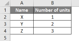
Step 1: Consider the same table which we took in the above example. Now we need to insert a column in between the two columns.
Step 2: A column will always be added on the left-hand side; hence select any one cell in the number of units as below.
Step 3: Now select the “Entire column” option from the insert option as shown in the below image.
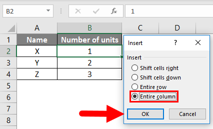
Step 4: Select the OK button. A new column will be added in between the existing two columns as below.
In a similar way, we can add the row by clicking the Entire row option as below.
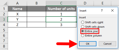
The result will be as below. A new row is added between the data X and Y.
Example #3 – Adding Rows After Each Row using the Sort Option
Up to now, we covered how to add a single cell by shifting cells right and down, adding an entire row an entire column.
But these actions will affect only one row or one column. In case if we want to add an empty row under each existing row, we can perform in another way. Follow the below steps to add an empty row.
Step 1: Take the same table which we used in the previous example.
Step 2: Take some reference for the time being column ‘C’ as below.
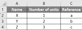
Step 3: Now copy the references and paste them in under the last reference in the table as below.
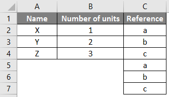
Step 4: To add an empty line under each existing data line, we are using a sorting option. Highlight the entire table and click on the sort option. It is available under “Home”, highlighted in the below picture for reference.
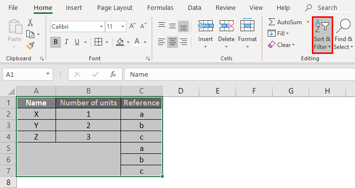
Step 5: From the drop-down of the Sort option, select the custom sort.
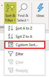
Step 6: A window will open as below.
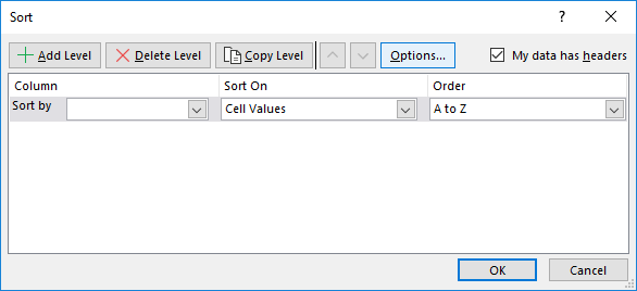
Step 7: From Sort by select the “Reference” option as shown in the below image.
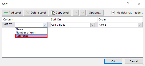
Step 8: Select OK, then see it will sort in such an empty line between each data existing line as below.
Step 9: Now, we can remove the reference column. I hope you understand why we added the reference column.
Example #4 – Adding Multiple Rows or Columns or Cells
If we want to add multiple lines or cells at the same time, highlight the number of cells or lines that you required and perform the insert option as per selection. If we select the multiple row lines as below.
Now use the insert option, which we add for rows.
The moment we select “insert cells”, it will directly add the rows without asking for another pop-up as how it asked before. Here we highlighted 3 lines; hence when we click on “Insert Cells”, it will add another 3 empty lines under the selected lines.
Things to Remember
- “Alt + I” is the shortcut key to add a cell or line in the excel spreadsheet.
- A new cell can be added only on the right-hand side and down only. We cannot add the cells to the left and up; hence whenever you want to add the cells to highlight the cell as per this rule.
- A row will always be added at the bottom of the highlighted cell.
- A column will always be added on the left side of the highlighted cell.
- If you want to add multiple cells or rows at a time, highlight multiple cells or rows.
Recommended Articles
This is a guide on How to Add Cells in Excel. Here we discuss How to Add Cells along with examples and downloadable excel template. You may also look at the following articles to learn more –
- How to Sum Multiple Rows in Excel
- SUM Cells in Excel
- Count Cells with Text in Excel
- Excel Shortcut For Merge Cells
Adding New Columns
Columns can be added and deleted. You access the menu by right clicking the column letter. New columns are added to the same place you clicked.
Let’s try to create a new column B.
Right click on the column and select «Insert Columns»:
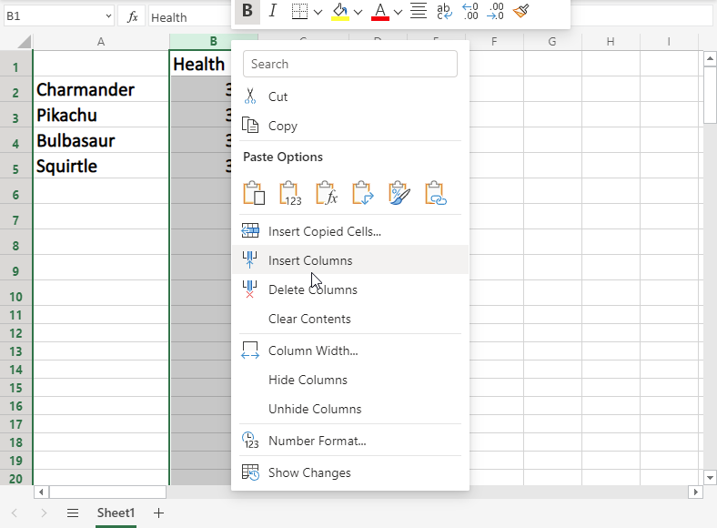
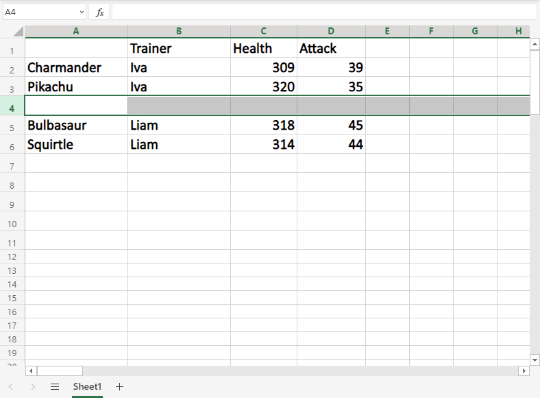
And a new column is created:

Next, we need to get some Pokemon trainers in there. Type or copy the following data in the new column B:
Adding New Rows
Rows can also be added and deleted. You access the menu by right clicking the row number. New rows are added to the same place you clicked.
Let’s try to create a new row 4.
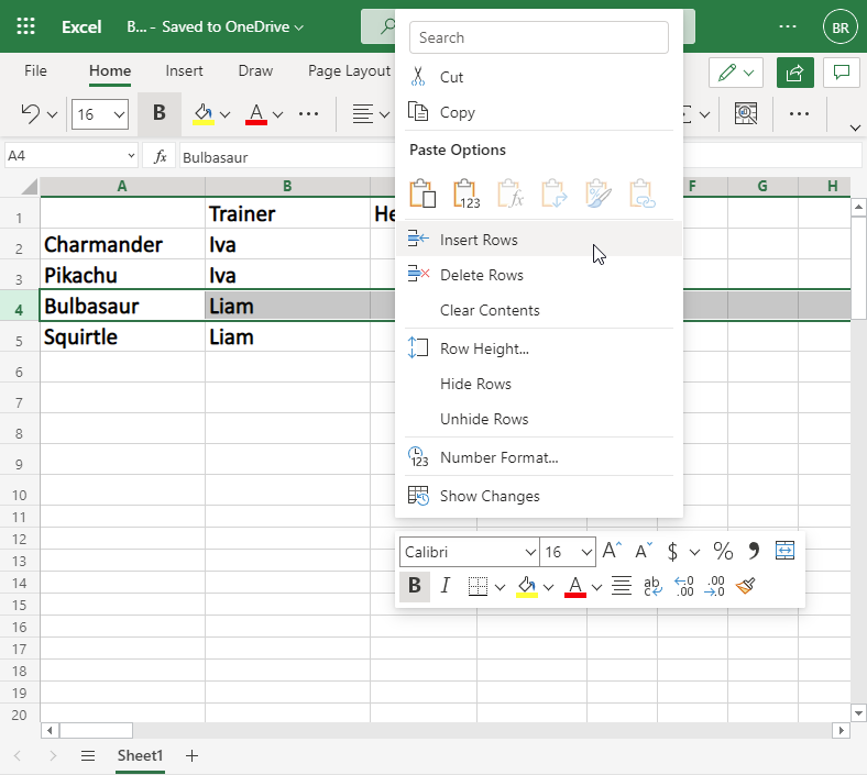
We forgot to add Iva’s Pokemon, Marowak. Lets add his data to the new row 4, by typing or copying the following values:
Excellent job!