Create calendars in excel

A calendar in Microsoft Excel comes in handy if you’ve a busy schedule. Although an Excel calendar is an outstanding tool that can assist you to stay prepared when it comes to vital events, appointments, activities, meetings, etc. Therefore, today we are here to discuss how to create calendar in Excel or how to insert calendar in Excel effortlessly.

So, without any further ado, let’s get started…

If you want to keep your data in a more organized way then a proper calendar system is very important for the right time management. Luckily Excel offers different ways to create calendars. Let’s know about each of them one by one in detail.

Method 1: Insert Calendar In Excel Using Date Picker Control

Well putting the drop-down calendar in Excel is quite easy to do but just because the time and date picker control are hidden so many users don’t know where it actually exists.

Here is the complete method to create a calendar in Excel perform this task step by step:

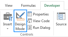
1. Enable The Developer Tab on Excel ribbon.

Excel date picker control actually belongs to the ActiveX controls family, which comes under the Developer tab. Though this Excel Developer tab is kept hidden you can enable its visibility.

• On the Excel ribbon, you have to make a right-click, and after that choose the option Customize the Ribbon…. This will open the Excel options.
• From the opened window go to the right-hand side section. Now from customizing the ribbon section, you have to select the Main Tabs. In the appearing main tab list check the Developer box option and then click the OK button.

Also Read: How to Create a Flowchart in Excel? (Step-By-Step Guide)

1. Insert The Calendar Control

Well, the Excel drop-down calendar is technically known as Microsoft Date and Time Picker Control.

To apply this in the Excel sheet, perform the following steps:

• Hit the Developer tab and then from the Controls group, you have to make a tap over arrow sign present within the Insert tab.

Now from the ActiveX Controls choose the “More Controls” button.

• From the opened dialog box of More Controlsselect the Microsoft Date and Time Picker Control 6.0 (SP6). After that click to the OK

• Hit the cell, in which you have to enter the calendar control.

You will see that a drop-down calendar control starts appearing on your Excel sheet:

Once this date picker control is been inserted, you will see that the EMBED formula starts appearing within the formula bar.

This gives detail to your Excel application about what kind of control is embedded within the sheet. You can’t change edit or delete this control because this will show the error “Reference is not valid“.

Adding the ActiveX control such date picker automatically enables the design mode which will allow you to change the properties and appearance of any freshly added control. The most obvious modification that you need to make at this time is resizing the calendar control and then linking it back to any specific cell.

For activating the Excel drop-down calendar option, hit the Design tab, and then from the Controls group, disable the Design Mode:

• Now, make a tap over the drop-down arrow for showing up the calendar and then select the date as per your need.
• Click the dropdown arrow to show the calendar in Excel and choose your desired date.

Note:

If MS date picker control is now not available within the list of More Controls. This situation mainly arises due to the following reasons.

• While you are running the MS Office 64 bit version. As there is no official date picker control available in the Office 64-bit.
• Calendar control i.e mscomct2.ocx is now not present or it is not registered on your PC.

1. Customize Calendar Control

After the addition of the calendar control on your Excel sheet, now you have to shift this calendar control on the desired location and then resize it to get an easy fit within a cell.

• For resizing this date picker control, you have to enable the Design Mode after that drag this control from the corner section:

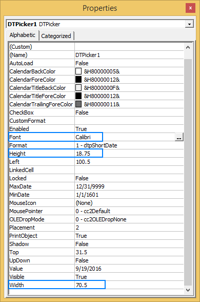
Or else you after enabling the Design Mode on, from the calendar control group choose the Properties tab:

• From the opened Properties window, you have to set the desired width, height, font size and style:

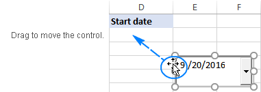
• To shift the Excel date picker control, place your mouse pointer over that and when the cursor changes into a four-pointed arrow sign, just drag the object wherever you want to place it.

1. Link Excel Calendar Control With The Cell

After successfully adding the calendar drop-down in excel, you need to link it with some specific cell. This step very compulsory to perform if you want to make use of any selected dates with the formulas.

Suppose you are writing the formula for counting up the order’s number between any specific dates. For stopping any other from entering wrong dates such as 2/30/2016 you have inserted a drop-down calendar within 2 cells.

The COUNTIF formula that you have applied for calculating a number of orders will return the value “0” even if the orders are present.

Well, the main reason can be that your Excel is unable to recognize the value present in the date picker control. This problem will persist until you link the control with some specific cell. Here is the step that you need to perform:

1. Selecting the calendar control you have to enable the Design Mode.
2. Go to the Developer tab and then from the control group tap to the
3. In the opened “Properties” windows, assign cell reference in the LinkedCell property (here I have written A3):

If Excel shows the following error “Can’t set cell value to NULL…” then click the OK button to ignore this.

After selecting the date from the drop-down calendar, the date will immediately start appearing in the linked cell. Now excel won’t face any issue in understanding the dates and the formula referencing done in the linked cells will work smoothly.

If you don’t need to have extra dates then link the date picker control with the cells where they are present.

Also Read: 4 Ways To Create Drop-Down List In Excel

Method 2: Using Excel Calendar Template

In Excel, there are handy graphic options with the clipart, tables, drawing tools, charts, etc. Using these options one can easily create a monthly calender or weekly calendar with special occasion dates or photos.

So go with the Excel calendar template which is the fastest and easiest way to create calendar in Excel using worksheet data.

Here are the steps to create calendar from Excel spreadsheet data using the template.

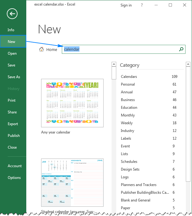
• Click the File> New after that in the search box you have to type “calendar”.
• Excel will make search thousands of online templates and then shows you the selected calendar templates which are grouped into the following categories.

• Choose the calendar template as per your requirement, and then tap to the Create.

That’s all you need to do…!

Excel calendar template will be opened from the new Excel workbook and then print or customize as per your need.  Usually, Excel weekly calendar templates are set with a year, whereas in some templates you can set a day for starting a week.

Note: for displaying always the current year in your excel calendar just assign a simple formula like this in the cell of the year: =YEAR(TODAY())

In this way, you can easily insert the drop-down calendar. Also, you can make a printable Excel calendar.

Method 3: Create Calendar In Excel Using VBA Code

In this method, you will get know-how using the Visual Basic for Applications(VBA) macro code you can create calendar in Excel.

1. Open your Excel workbook.
2. For excel 2003 users: Go to the Tools menu, and then hit the Macro tab. After that choose the Visual Basic Editor.

For Excel 2007 or later users: go to the Developer tab from the Excel ribbon and choose Visual Basic.

1. From the Insert menu, choose the Module option.
2. Now paste the VBA code which is given below into the opened sheet of the module.
3. Go to the File menu and choose the Close and Return to Microsoft Excel.
4. Now make a selection of the Sheet1
5. From the Tools menu, go to the Macro tab. After that choose the Macros icon.
6. Now you have to choose the CalendarMaker Now press the Run button to create Excel calendar.

Visual Basic Procedure To Create a Calendar In Excel:

You have to paste this code in the module sheet.

Note: You can customize the above code as per your requirement.

How Do I Make Excel Calendar Update Automatically?

Automatization is the chief strength of Microsoft Excel. However, if you need to create your calendar update automatically then use the formula mentioned below:

“= EOMONTH (TODAY() , – 1) +1”.

Well, the above formula employs “TODAY” feature to locate the present date & calculates the 1^st day of the month with the “EOMONTH” feature.

Related FAQs:

Also Read: How To Create Backup Of Active Workbooks In Excel?

Wrap Up:

MS Excel offers its user a broad range of tools which will increase their productivity by using the projects, dates, and tracking events. In order to view the data of your Excel worksheet in calendar format, Microsoft will change your data and then import it into the Outlook. This will automatically change it into a calendar format.

Hopefully, you must have found an ample amount of information in this post. Thanks for reading this post….!

Is this article up to date?

При создании таблиц с определенным типом данных иногда нужно применять календарь. Кроме того, некоторые пользователи просто хотят его создать, распечатать и использовать в бытовых целях. Программа Microsoft Office позволяет несколькими способами вставить календарь в таблицу или на лист. Давайте выясним, как это можно сделать.

Если инструкция по созданию календаря в Microsoft Excel вам покажется сложной, в качестве альтернативы рекомендуем рассмотреть веб-платформу Canva, доступную онлайн из любого браузера. Это сервис с огромной библиотекой редактируемых шаблонов различной направленности и стилистики, в числе которых есть и календари. Любой из них можно изменить на свое усмотрение либо создать таковой с нуля и затем сохранить на компьютер в предпочтительном формате или распечатать.

Создание различных календарей

Все календари, созданные в Excel, можно разделить на две большие группы: охватывающие определенный отрезок времени (например, год) и вечные, которые будут сами обновляться на актуальную дату. Соответственно и подходы к их созданию несколько отличаются. Кроме того, можно использовать уже готовый шаблон.

Способ 1: создание календаря на год

Прежде всего, рассмотрим, как создать календарь за определенный год.

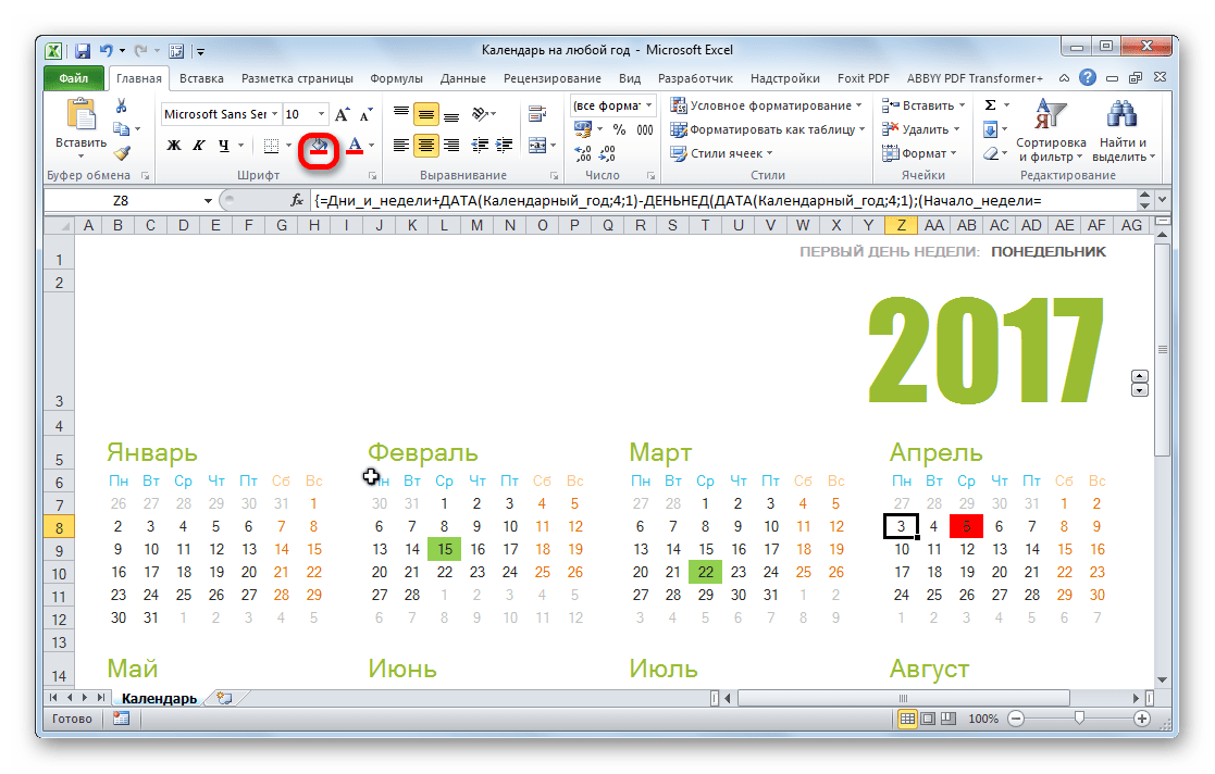
1. Разрабатываем план, как он будет выглядеть, где будет размещаться, какую ориентацию иметь (альбомную или книжную), определяем, где будут написаны дни недели (сбоку или сверху) и решаем другие организационные вопросы.
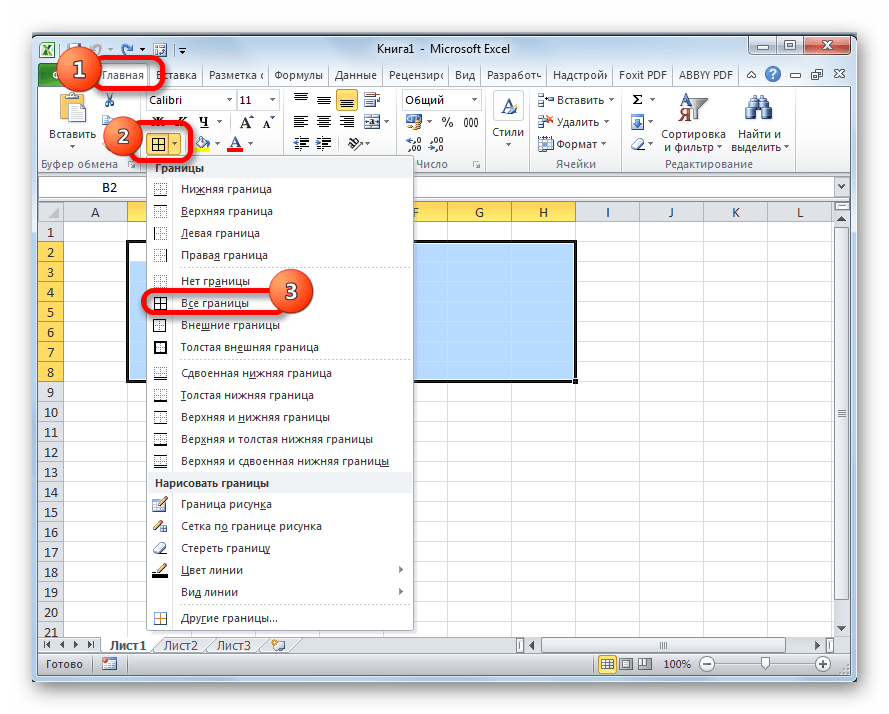
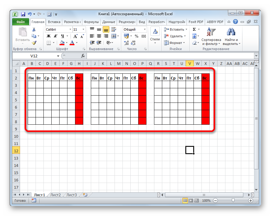
2. Для того, чтобы сделать календарь на один месяц выделяем область, состоящую из 6 ячеек в высоту и 7 ячеек в ширину, если вы решили писать дни недели сверху. Если вы будете их писать слева, то, соответственно, наоборот. Находясь во вкладке «Главная», кликаем на ленте по кнопке «Границы», расположенной в блоке инструментов «Шрифт». В появившемся списке выбираем пункт «Все границы».



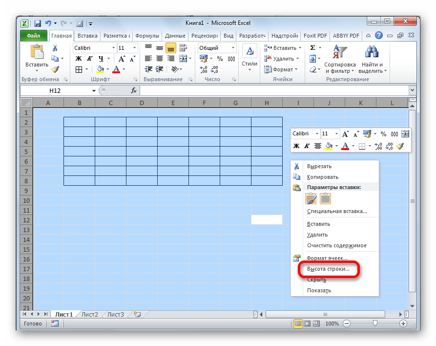
3. Выравниваем ширину и высоту ячеек, чтобы они приняли квадратную форму. Для того, чтобы установить высоту строки кликаем на клавиатуре сочетание клавиш Ctrl+A. Таким образом, выделяется весь лист. Затем вызываем контекстное меню кликом левой кнопки мыши. Выбираем пункт «Высота строки».
   

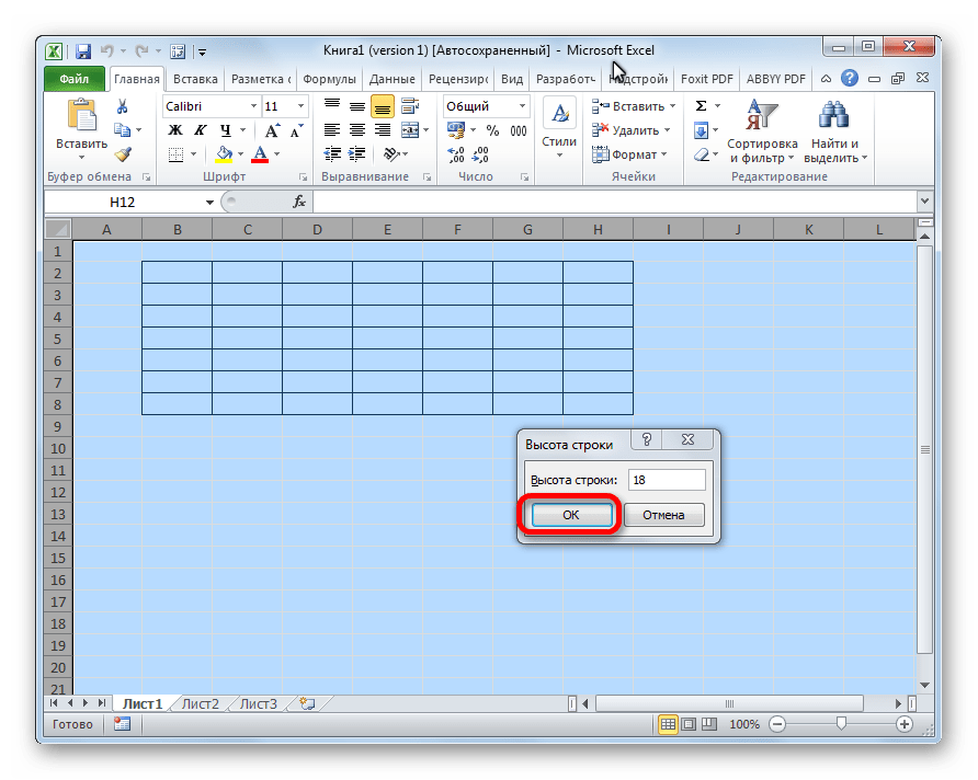
   Открывается окно, в котором нужно установить требуемую высоту строки. Ели вы впервые делаете подобную операцию и не знаете, какой размер установить, то ставьте 18. Потом жмите на кнопку «OK».

   

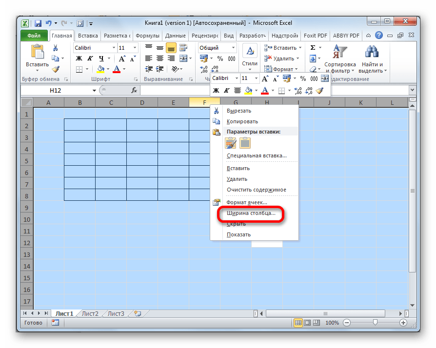
   Теперь нужно установить ширину. Кликаем по панели, на которой указаны наименования столбцов буквами латинского алфавита. В появившемся меню выбираем пункт «Ширина столбцов».

   

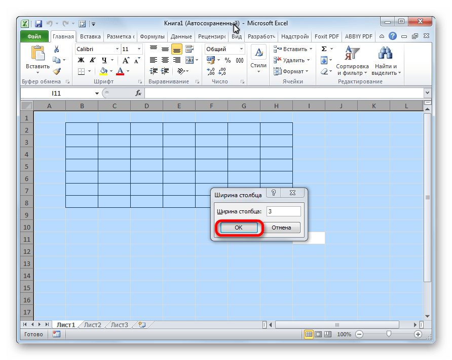
   В открывшемся окне установите нужный размер. Если не знаете, какой размер установить, можете поставить цифру 3. Жмите на кнопку «OK».

   

   После этого, ячейки на листе приобретут квадратную форму.

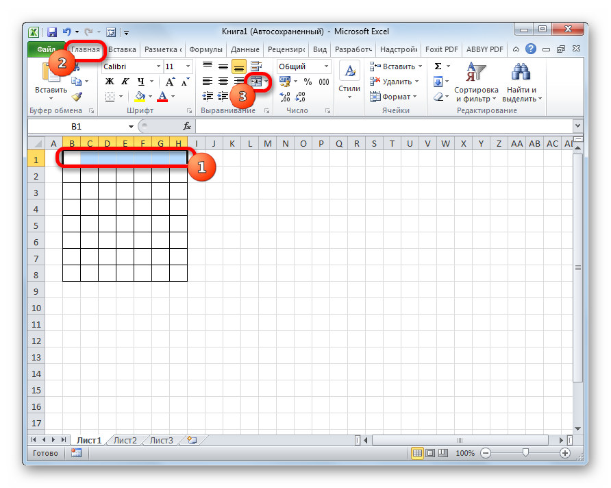
4. Теперь над расчерченным шаблоном нам нужно зарезервировать место для названия месяца. Выделяем ячейки, находящиеся выше строки первого элемента для календаря. Во вкладке «Главная» в блоке инструментов «Выравнивание» жмем на кнопку «Объединить и поместить в центре».



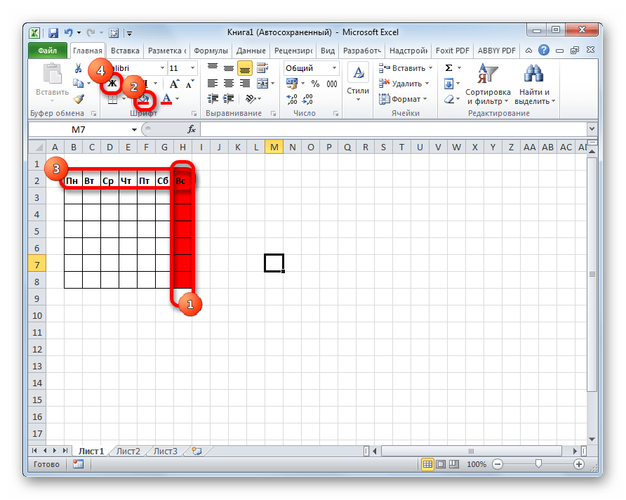
5. Прописываем дни недели в первом ряду элемента календаря. Это можно сделать при помощи автозаполнения. Вы также можете на свое усмотрение отформатировать ячейки этой небольшой таблицы, чтобы потом не пришлось форматировать каждый месяц в отдельности. Например, можно столбец, предназначенный для воскресных дней залить красным цветом, а текст строки, в которой находятся наименования дней недели, сделать полужирным.





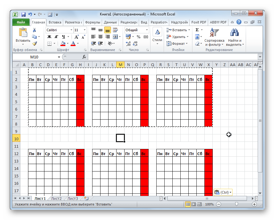
6. Копируем элементы календаря ещё для двух месяцев. При этом не забываем, чтобы в область копирования также входила объединенная ячейка над элементами. Вставляем их в один ряд так, чтобы между элементами была дистанция в одну ячейку.



7. Теперь выделяем все эти три элемента, и копируем их вниз ещё в три ряда. Таким образом, должно получиться в общей сложности 12 элементов для каждого месяца. Дистанцию между рядами делайте две ячейки (если используете книжную ориентацию) или одну (при использовании альбомной ориентации).



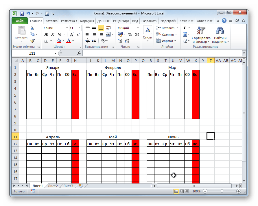
8. Затем в объединенной ячейке пишем название месяца над шаблоном первого элемента календаря – «Январь». После этого, прописываем для каждого последующего элемента своё наименование месяца.



9. На заключительном этапе проставляем в ячейки даты. При этом, можно значительно сократить время, воспользовавшись функцией автозаполнения, изучению которой посвящен отдельный урок.

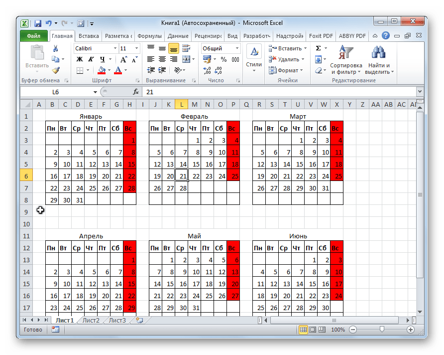
После этого, можно считать, что календарь готов, хотя вы можете дополнительно отформатировать его на своё усмотрение.

Урок: Как сделать автозаполнение в Excel

Способ 2: создание календаря с использованием формулы

Но, все-таки у предыдущего способа создания есть один весомый недостаток: его каждый год придется делать заново. В то же время, существует способ вставить календарь в Excel с помощью формулы. Он будет каждый год сам обновляться. Посмотрим, как это можно сделать.

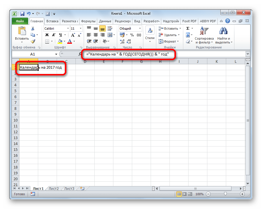
1. В левую верхнюю ячейку листа вставляем функцию:
   ="Календарь на " & ГОД(СЕГОДНЯ()) & " год"
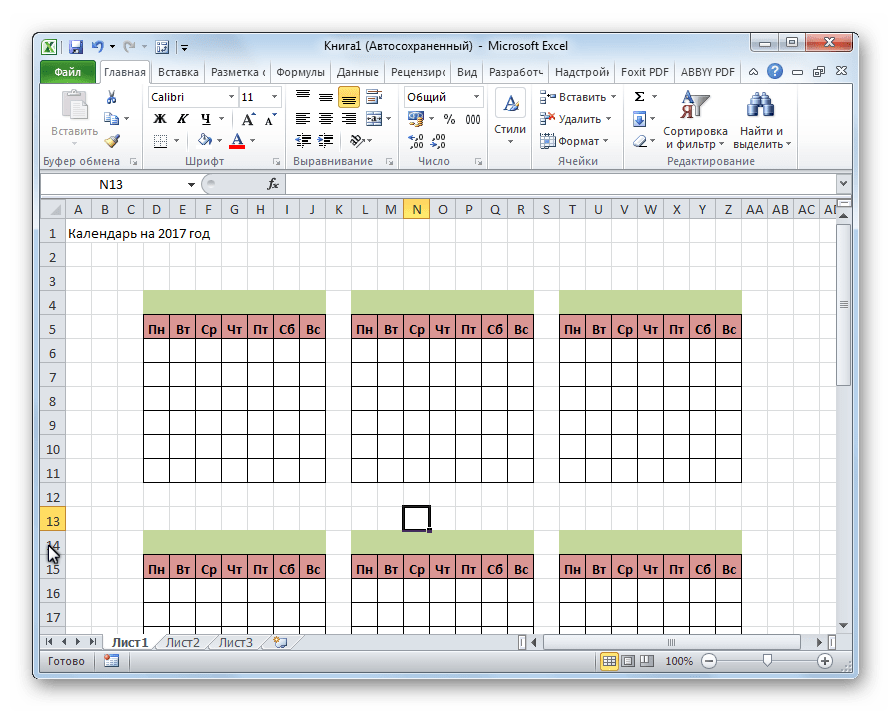
   Таким образом, мы создаем заголовок календаря с текущим годом.



2. Чертим шаблоны для элементов календаря помесячно, так же как мы это делали в предыдущем способе с попутным изменением величины ячеек. Можно сразу провести форматирование этих элементов: заливка, шрифт и т.д.



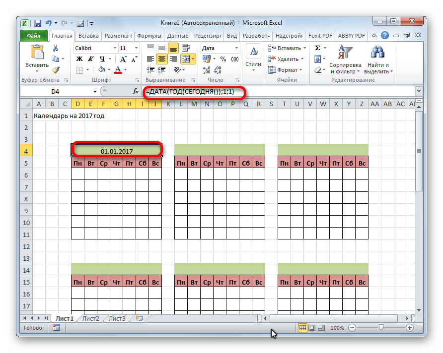
3. В место, где должно отображаться названия месяца «Январь», вставляем следующую формулу:
   =ДАТА(ГОД(СЕГОДНЯ());1;1)
   

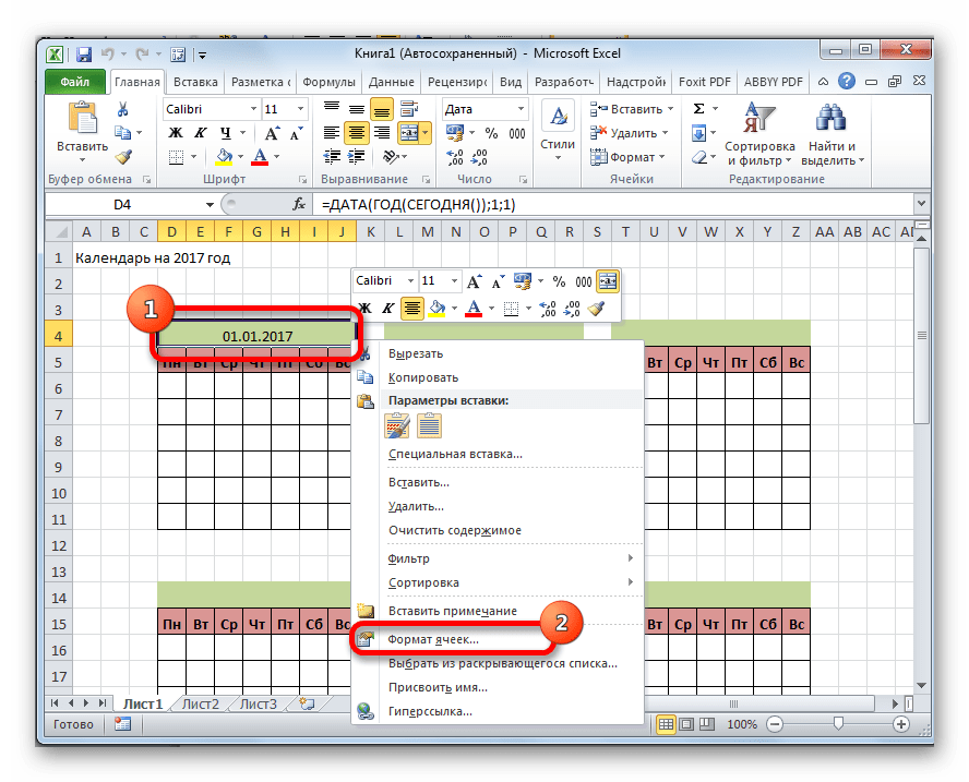
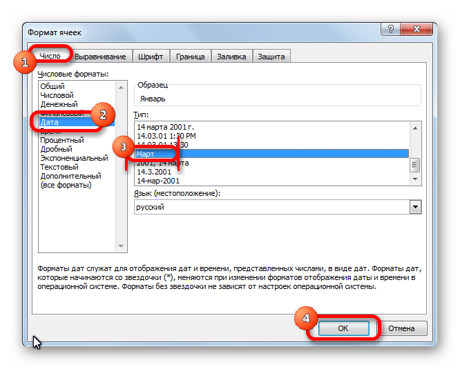
   Но, как видим, в том месте, где должно отобразиться просто название месяца установилась дата. Для того, чтобы привести формат ячейки к нужному виду, кликаем по ней правой кнопкой мыши. В контекстном меню выбираем пункт «Формат ячеек…».

   

   В открывшемся окне формата ячеек переходим во вкладку «Число» (если окно открылось в другой вкладке). В блоке «Числовые форматы» выделяем пункт «Дата». В блоке «Тип» выбираем значение «Март». Не беспокойтесь, это не значит, что в ячейке будет слово «Март», так как это всего лишь пример. Жмем на кнопку «OK».



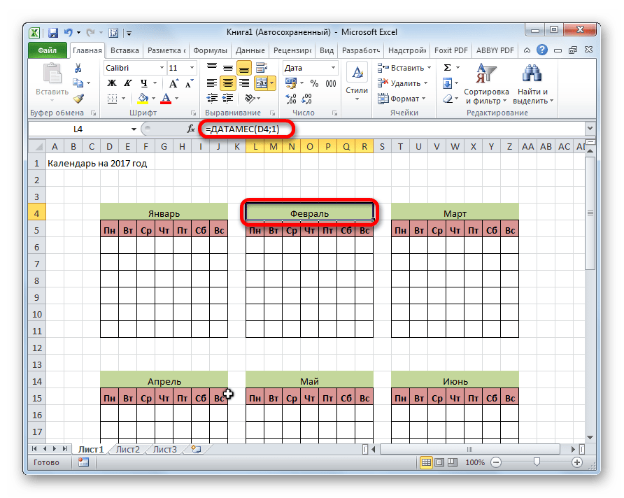
4. Как видим, наименование в шапке элемента календаря изменилось на «Январь». В шапку следующего элемента вставляем другую формулу:
   =ДАТАМЕС(B4;1)
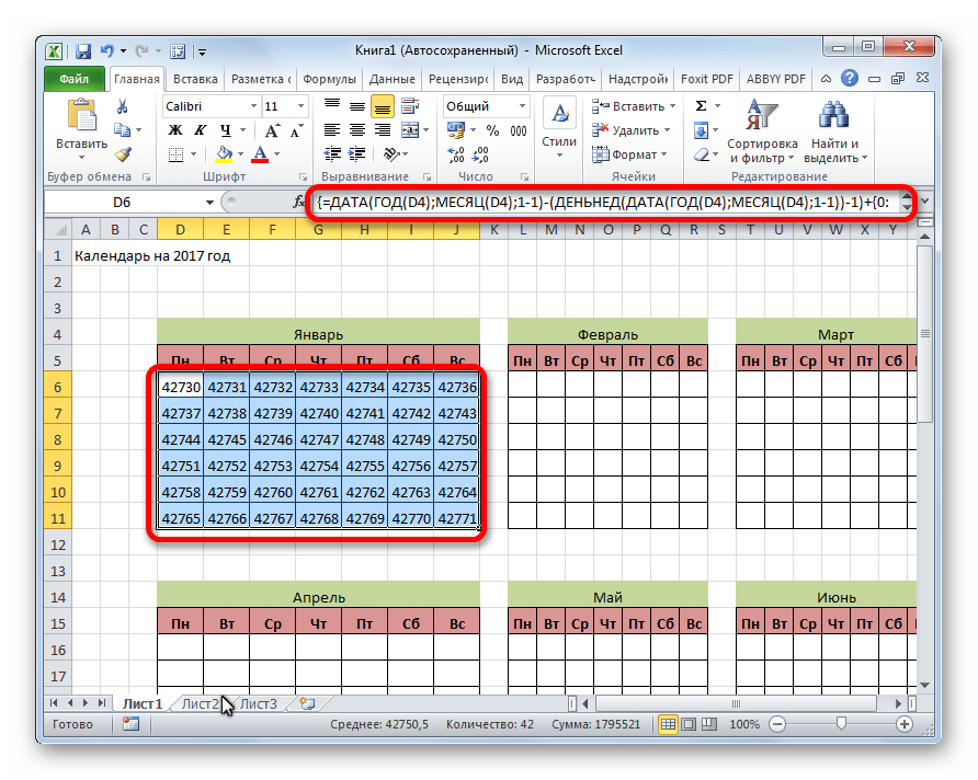
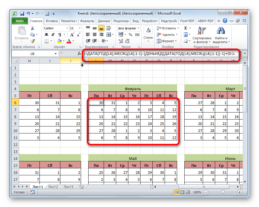
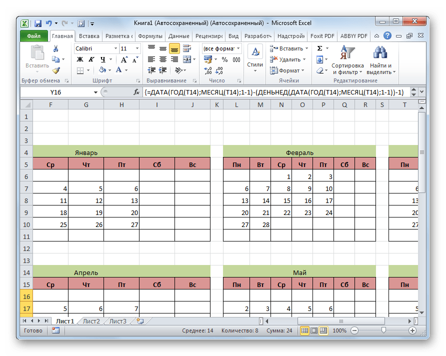
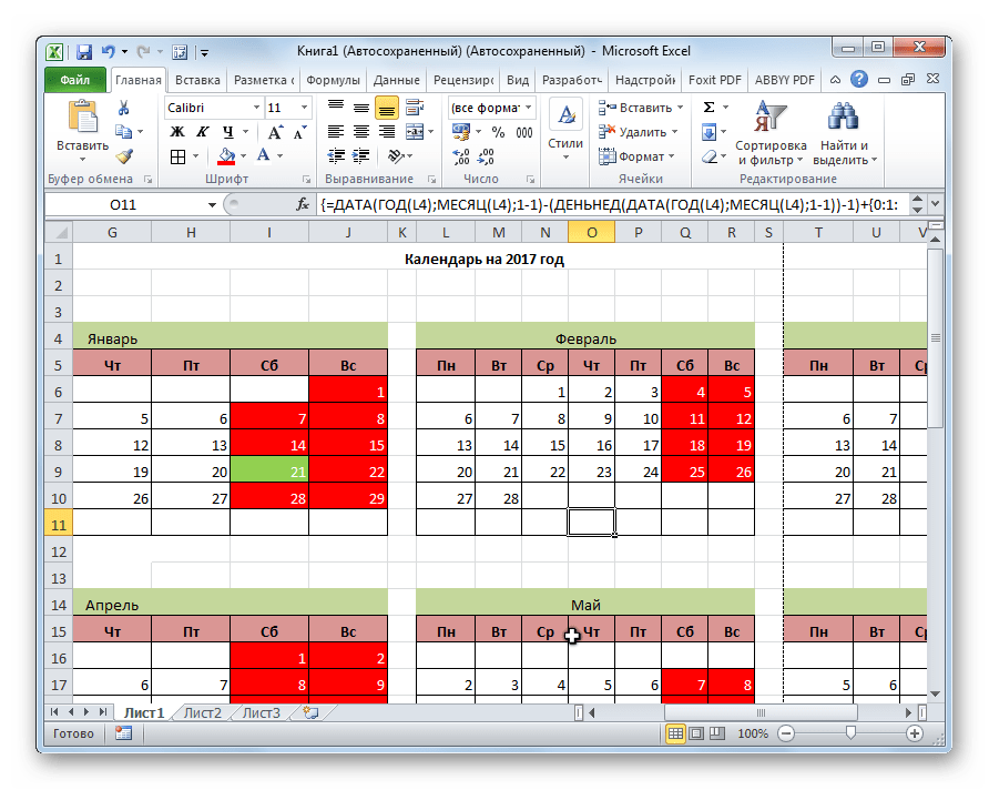
   В нашем случае, B4 – это адрес ячейки с наименованием «Январь». Но в каждом конкретном случае координаты могут быть другими. Для следующего элемента уже ссылаемся не на «Январь», а на «Февраль», и т.д. Форматируем ячейки так же, как это было в предыдущем случае. Теперь мы имеем наименования месяцев во всех элементах календаря.



5. Нам следует заполнить поле для дат. Выделяем в элементе календаря за январь все ячейки, предназначенные для внесения дат. В Строку формул вбиваем следующее выражение:
   =ДАТА(ГОД(D4);МЕСЯЦ(D4);1-1)-(ДЕНЬНЕД(ДАТА(ГОД(D4);МЕСЯЦ(D4);1-1))-1)+{0:1:2:3:4:5:6}*7+{1;2;3;4;5;6;7}
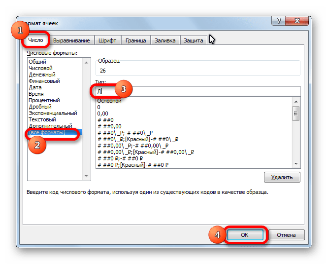
   Жмем сочетание клавиш на клавиатуре Ctrl+Shift+Enter.



6. Но, как видим, поля заполнились непонятными числами. Для того, чтобы они приняли нужный нам вид. Форматируем их под дату, как это уже делали ранее. Но теперь в блоке «Числовые форматы» выбираем значение «Все форматы». В блоке «Тип» формат придется ввести вручную. Там ставим просто букву «Д». Жмем на кнопку «OK».



7. Вбиваем аналогичные формулы в элементы календаря за другие месяцы. Только теперь вместо адреса ячейки D4 в формуле нужно будет проставить координаты с наименованием ячейки соответствующего месяца. Затем, выполняем форматирование тем же способом, о котором шла речь выше.



8. Как видим, расположение дат в календаре все ещё не корректно. В одном месяце должно быть от 28 до 31 дня (в зависимости от месяца). У нас же в каждом элементе присутствуют также числа из предыдущего и последующего месяца. Их нужно убрать. Применим для этих целей условное форматирование.

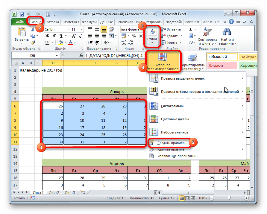
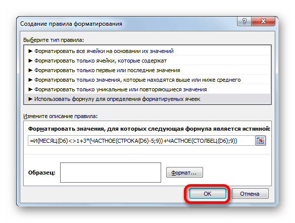
   Производим в блоке календаря за январь выделение ячеек, в которых содержатся числа. Кликаем по значку «Условное форматирование», размещенному на ленте во вкладке «Главная» в блоке инструментов «Стили». В появившемся перечне выбираем значение «Создать правило».

   

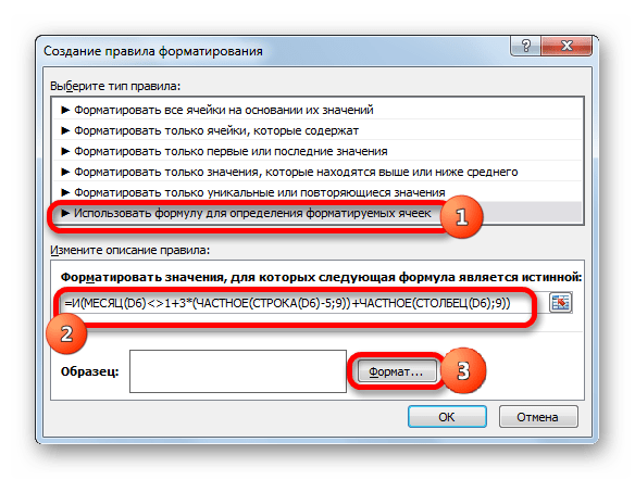
   Открывается окно создания правила условного форматирования. Выбираем тип «Использовать формулу для определения форматируемых ячеек». В соответствующее поле вставляем формулу:
   =И(МЕСЯЦ(D6)1+3*(ЧАСТНОЕ(СТРОКА(D6)-5;9))+ЧАСТНОЕ(СТОЛБЕЦ(D6);9))
   D6 – это первая ячейка выделяемого массива, который содержит даты. В каждом конкретном случае её адрес может отличаться. Затем кликаем по кнопке «Формат».

   

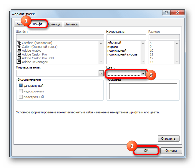
   В открывшемся окне переходим во вкладку «Шрифт». В блоке «Цвет» выбираем белый или цвет фона, если у вас установлен цветной фон календаря. Жмем на кнопку «OK».

   

   Вернувшись в окно создания правила, жмем на кнопку «OK».



9. Используя аналогичный способ, проводим условное форматирование относительно других элементов календаря. Только вместо ячейки D6 в формуле нужно будет указывать адрес первой ячейки диапазона в соответствующем элементе.



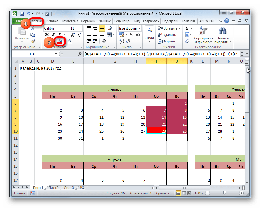
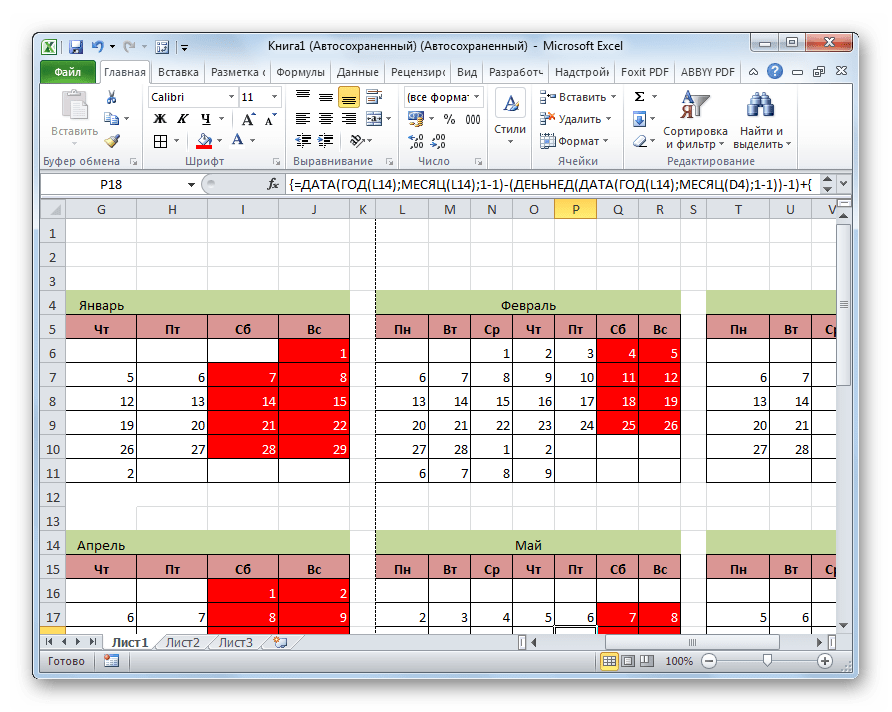
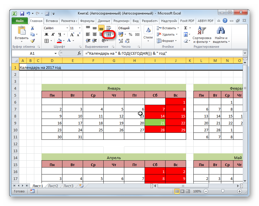
10. Как видим, числа, которые не входят в соответствующий месяц, слились с фоном. Но, кроме того, с ним слились и выходные дни. Это было сделано специально, так как ячейки, где содержаться числа выходных дней мы зальём красным цветом. Выделяем в январском блоке области, числа в которых выпадают на субботу и воскресение. При этом, исключаем те диапазоны, данные в которых были специально скрыты путем форматирования, так как они относятся к другому месяцу. На ленте во вкладке «Главная» в блоке инструментов «Шрифт» кликаем по значку «Цвет заливки» и выбираем красный цвет.
    

    Точно такую же операцию проделываем и с другими элементами календаря.



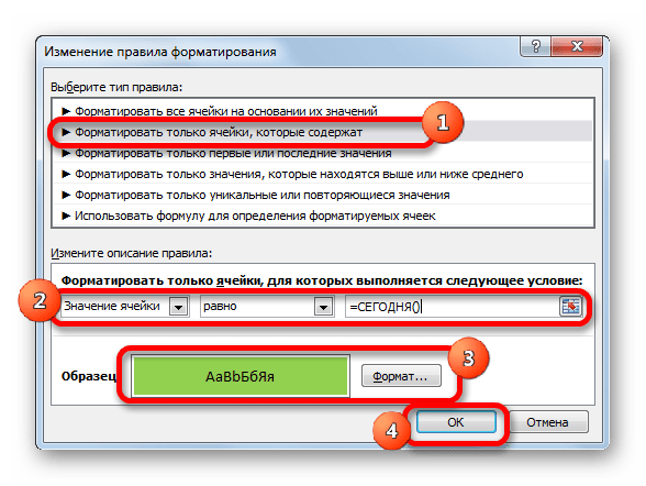
11. Произведем выделение текущей даты в календаре. Для этого, нам нужно будет опять произвести условное форматирование всех элементов таблицы. На этот раз выбираем тип правила «Форматировать только ячейки, которые содержат». В качестве условия устанавливаем, чтобы значение ячейки было равно текущему дню. Для этого вбиваем в соответствующее поля формулу (показано на иллюстрации ниже).
    =СЕГОДНЯ()
    В формате заливки выбираем любой цвет, отличающийся от общего фона, например зеленый. Жмем на кнопку «OK».
    

    После этого, ячейка, соответствующая текущему числу, будет иметь зеленый цвет.

12. Установим наименование «Календарь на 2017 год» посередине страницы. Для этого выделяем всю строку, где содержится это выражение. Жмем на кнопку «Объединить и поместить в центре» на ленте. Это название для общей презентабельности можно дополнительно отформатировать различными способами.

В целом работа над созданием «вечного» календаря завершена, хотя вы можете ещё долго проводить над ним различные косметические работы, редактируя внешний вид на свой вкус. Кроме того, отдельно можно будет выделить, например, праздничные дни.

Урок: Условное форматирование в Excel

Способ 3: использование шаблона

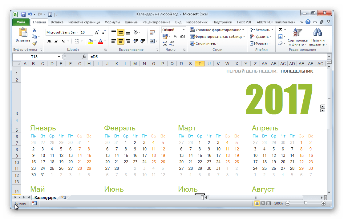
Те пользователи, которые ещё в недостаточной мере владеют Экселем или просто не хотят тратить время на создание уникального календаря, могут воспользоваться готовым шаблоном, закачанным из интернета. Таких шаблонов в сети довольно много, причем велико не только количество, но и разнообразие. Найти их можно, просто вбив соответствующий запрос в любую поисковую систему. Например, можно задать следующий запрос: «календарь шаблон Excel».

Примечание: В последних версиях пакета Microsoft Office огромный выбор шаблонов (в том числе и календарей) интегрирован в состав программных продуктов. Все они отображаются непосредственно при открытии программы (не конкретного документа) и, для большего удобства пользователя, разделены на тематические категории. Именно здесь можно выбрать подходящий шаблон, а если такового не найдется, его всегда можно скачать с официального сайта Office.com.

По сути, такой шаблон — уже готовый календарь, в котором вам только останется занести праздничные даты, дни рождения или другие важные события. Например, таким календарем является шаблон, который представлен на изображении ниже. Он представляет собой полностью готовую к использованию таблицу.

Вы можете в нем с помощью кнопки заливки во вкладке «Главная» закрасить различными цветами ячейки, в которых содержатся даты, в зависимости от их важности. Собственно, на этом вся работа с подобным календарем может считаться оконченной и им можно начинать пользоваться.

Мы разобрались, что календарь в Экселе можно сделать двумя основными способами. Первый из них предполагает выполнение практически всех действий вручную. Кроме того, календарь, сделанный этим способом, придется каждый год обновлять. Второй способ основан на применении формул. Он позволяет создать календарь, который будет обновляться сам. Но, для применения данного способа на практике нужно иметь больший багаж знаний, чем при использовании первого варианта. Особенно важны будут знания в сфере применения такого инструмента, как условное форматирование. Если же ваши знания в Excel минимальны, то можно воспользоваться готовым шаблоном, скачанным из интернета.

Excel is a powerful tool for crunching numbers. But it can also double as a fully-fledged calendar and planner, even if that means dumbing down its functionality a bit. In this article, you’ll learn how to make a calendar in Excel in three simple steps.

So, without further ado, let’s dive in. 👇

Table of Contents

1

🤔 What Is a Calendar in Excel?

A calendar in Excel lets you do pretty much what a regular calendar does:

• 👩‍⚕️ Schedule meetings and appointments.
• ✔️ Keep track of deadlines and important dates.
• 🎯 Set daily, weekly, and monthly goals.
• 🟢 Check your availability at a glance.
• 🗓️ Plan ahead and prepare for upcoming events.

Of course, there are also a few other gimmicks that come with the spreadsheet pedigree.

You can customize each and every worksheet cell to your heart’s content. Tweak one of the dozens of formatting options or apply conditional formatting and watch cells change appearance based on their contents. We’re not saying that you should, but it’s possible.

The options are limitless, and for our taste, a bit overwhelming.

Since we don’t have the time (or patience) for all that, let’s stick to the basics.

🏗️ How to Make a Calendar in Excel in 3 Steps

1. Use a Template or Start from Scratch

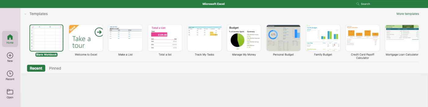
When you first open Excel, you have two choices. You can create a blank workbook and format the calendar yourself or pick one of the available templates to speed up the process. 

Choosing a ready-made framework is a no-brainer.

All you need to do is type “calendar” in the search bar in the top-right corner. There are dozens of pre-filled frameworks, each with unique styling and composition. 

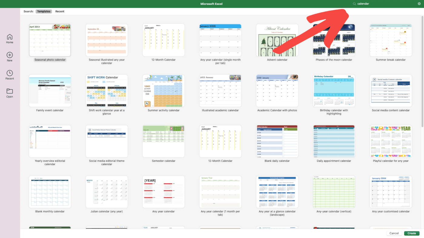
Using templates is faster, but it leaves you with limited customization options.

Let’s try a more hands-on approach. 💪

Pick the Blank Workbook option from the list at the top.

 [template]

Next, right-click “Sheet1” at the bottom, choose “Rename,” and type in the current month.

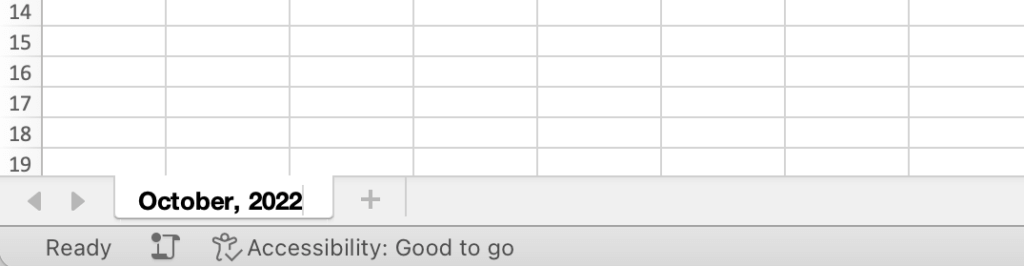
Great, moving on. 👉

2. Format Your Excel Calendar

Our spreadsheet is crisp and clear. But it doesn’t look anything like a monthly calendar.

Select seven columns at the top, from A to G and set Column Width to “20.” 

Repeat the step for rows 1 to 7 and set Row Height to “70.”

Our calendar is taking shape. Let’s give it some visual upgrades to make it look the part.

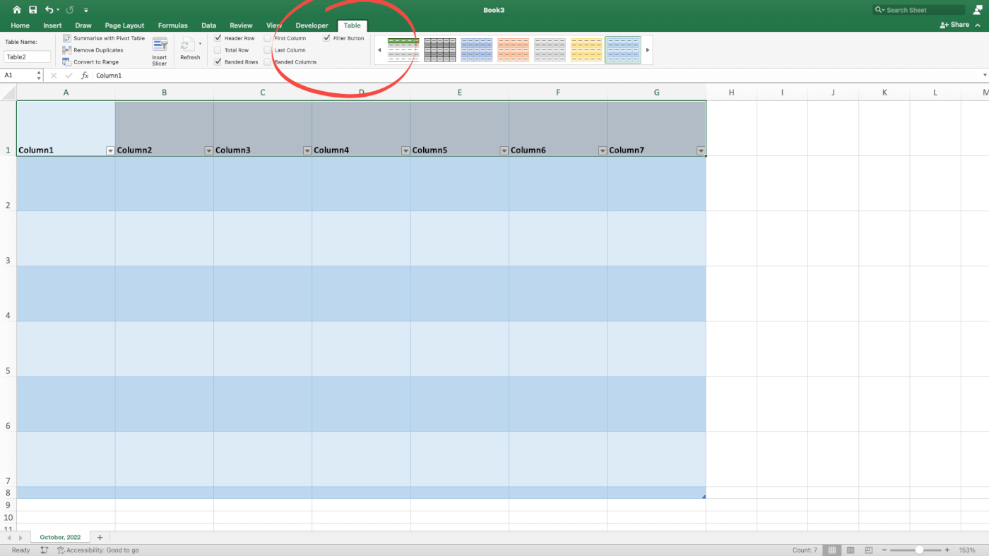
Select cells A1:G8, click Format as Table in the Home tab, and choose one of the available styles. To remove the ugly filter buttons at the top, go to Table and deselect “Filter Button.”

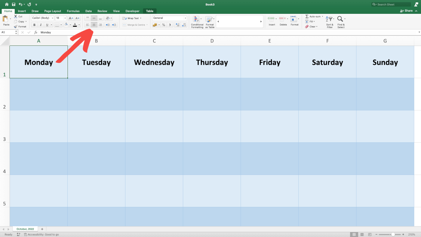
Finally, apply Align to Middle and Center Text to the top row of your table (cells A1:G1).

Now, you can add days of the week at the top of each column. Make sure to format the text so it’s easily readable. You can change the font style, size, and color.

All that’s left is to number the days in our calendar. You can use a wall calendar (or the one on your phone) for reference. When done, select the cells and top-align/right-align the text.

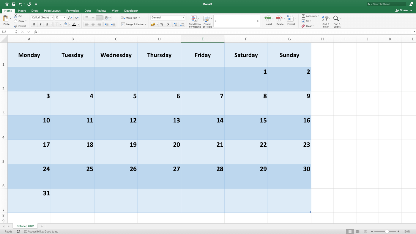
Now that you have a calendar template in place, you can create a few new sheets, one for each month, or duplicate the template to create a quarterly calendar in the same sheet.

3. Track Tasks and Events

Let’s put our new calendar to good use and start tracking monthly tasks.

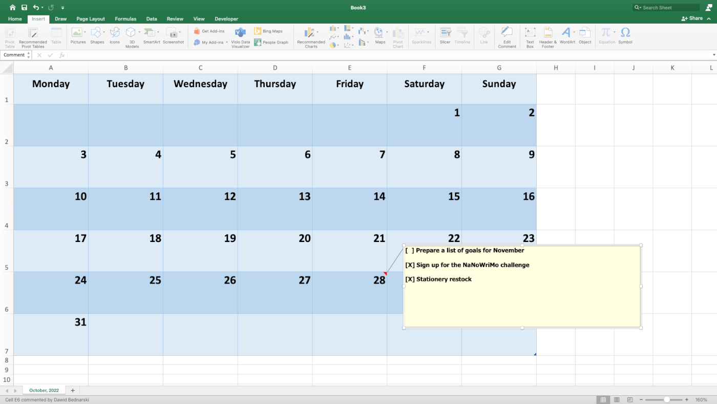
The simplest way to do that is the Comment feature.

Select the day when you want to schedule a task and click New Comment in the Insert tab at the top. Write down your tasks and events using bullets or square brackets. The second approach lets you mark each task as complete by adding an “X” inside the brackets.

⚡️ Pro Tip: Press ⌨️ Shift+F2 to quickly insert a comment.

We can’t say this is the best calendar experience we’ve seen, but what can you do? 🤷‍♂️

Well, you can try Taskade! 🥳

🐑 Create Easy to Use Calendars With Taskade

Taskade is a powerful and user-friendly task management tool for teams and individuals.

With Taskade, you don’t have to spend hours putting together a flaky calendar. You can set up a project and start getting work done in seconds instead of hours.

All that thanks to powerful features like:

• 🤏 Drag & drop workflow
• 👀 Dynamic project views
• 📱 Mobile and Desktop Apps
• 🏷 Task sorting and #hashtags
• 🔄 Recurring tasks
• 🔔 Custom notifications
• ⚡️ Real-time collaboration

And more!

Taskade is simple, intuitive, and fun. And that’s hardly something you can say about Excel or any other member of the Office family (sorry, not sorry).

But let’s get down to business.

Taskade lets you create and manage tasks and calendar events in three ways. 🤹‍♂️

1. The Calendar View

Every project in Taskade is a self-contained workspace. This means you can plan your week, manage your work, and keep track of tasks without shuffling multiple apps.

To open the monthly calendar view, click in the main dashboard. You can choose from one of the 300+ templates or create a blank project and customize everything.

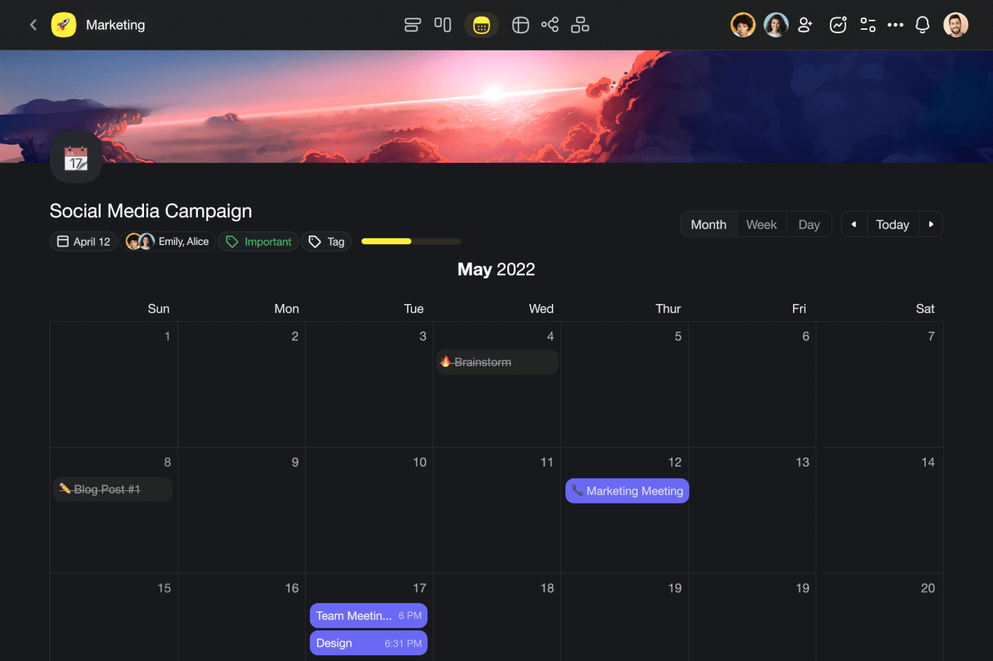
All you have to do now is click the Calendar View button in the top navigation bar.

By default, the calendar shows the current month, but you can move forward or backward using the buttons in the top-right corner. You can also switch to the Weekly or Daily view.

To schedule a new task or event, simply click a date and enter event details. Add event details, adjust time and date, and click to save changes.

2. Global Calendar

Let’s say you’re managing multiple projects, with different teams, tasks, roadmaps, and deadlines all mixed together. This is where our Global Calendar comes into play.

The Global Calendar shows you all tasks and events across all your projects within a Workspace or Folder. That means you can your finger on the pulse without shuffling multiple calendar apps.

Calnedar entries are color-coded, so you can easily distinguish between individual projects. Want to see the details of a task? Click the event and Taskade will instantly open the target project.

Finally, the Global Calendar lets you add tasks and notes to projects nested inside the parent Workspace or Folder. Simply choose a date, set the target, and enter the details of the task or note. The new entry will be instantly added to the target project.

3. Calendar Integrations

There are many to-do list and calendar apps that can help you stay on top of things.

But you don’t have to juggle multiple tools to do that. 🤹‍♂️

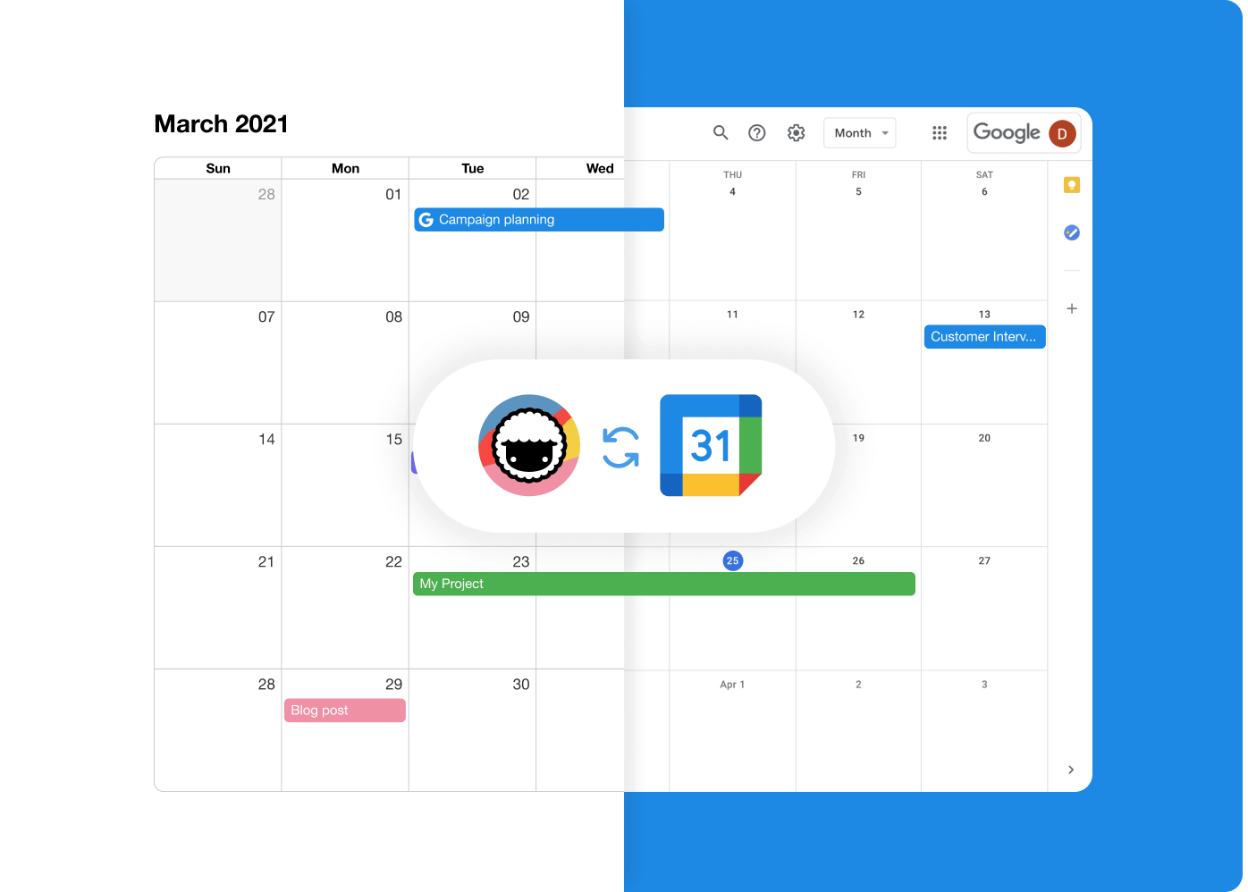
Taskade lets you sync with Outlook, iCloud, and Google calendars and see all your tasks and events in your calendar of choice. You can even enable two-way synchronization with the Google Calendar; all events you create will appear in the Taskade calendar in an instant.

Be sure to visit our Help Center to learn more about two-way Google synchronization.

And that’s it! 🥳 

💬 Frequently Asked Questions (FAQ)

Is there a calendar template on Excel?

Yes. Excel features an online template catalog with several calendar workflows you can import directly into the app. Templates in Excel let you organize spreadsheets into individual months, apply different visual styles, and insert additional components like task trackers or vacation planners.

Is there a 2022 calendar template in Excel?

All of the templates available for Microsoft Excel can be easily customized. You can import one of the existing templates from the template catalog and edit the number of days in each month for 2022. Another method is to run a quick Google search for “2022 Excel calendar templates” and pick one of the free and paid alternatives from third-party content creators.

What is the formula for a calendar in Excel?

There’s no easy way to insert a calendar into an Excel spreadsheet. You can, however, use Microsoft’s Visual Basic Editor and a macro formula that will auto-generate a calendar for you. You can download the formula from the official Microsoft Learn page.

Can you convert a spreadsheet to a calendar?

You can convert any Excel spreadsheet to a calendar using Microsoft’s Visual Basic script.

1. Create a blank Workbook.
2. Select Visual Basic in the Developer ribbon.
3. Go to the Insert menu and select Module.
4. Paste the Visual Basic script from the Microsoft Learn page.
5. Navigate to the File menu and click Close.
6. Select the Sheet1 tab.
7. Go to the Developer ribbon again and click Macros.
8. Select CalendarMaker and click Run to create the calendar.

How do I add a calendar to my spreadsheet?

Follow the steps below to quickly add a calendar to your spreadsheet:

1. Open Microsoft Excel and click New in the left navigation pane.
2. Type “calendar” in the search bar in the top-right corner.
3. Choose one of the available templates to create a calendar.

You can also start with a blank workbook and follow the tips from our article. Keep in mind that you’ll need to add dates and labels manually.

How do I create a recurring monthly schedule in Excel?

The bad news is that Excel doesn’t support recurring schedules out of the box. One workaround is to use a “=DATE” function to automatically generate consecutive days in the calendar based on the selected cells.

🐑 Conclusion

Excel is an impressive piece of software that can do much more than advertised.

But 9 times out of 10, the simplest solution is the best.

Taskade makes your life easier by simplifying planning and task management. You don’t have to spend hours building calendars from scratch. All the tools you need are just a click away!

So, what are you waiting for?

Make an appointment with Taskade (pun not intended) and sign up for a free account today. 👈

💡 Before you go… … Enjoyed the article? Be sure to check our article on how to create a to-do list in Excel next. You can also visit our YouTube channel for more project management insights.

Create a calendar for the week, month, or entire year.

Updated on September 23, 2022

What to Know

• Easiest way is to use the numerous pre-made calendar templates: Go to File > New > «calendar» in search field > select calendar > Create.
• Alternatively, use Excel to make a custom calendar.

This article explains four different ways on how to make a calendar in Excel. Instructions apply to Excel 2019, Excel 2016, Excel 2013, Excel 2010, Excel for Mac, Excel for Android, and Excel Online.

How to Make a Pre-Made Calendar in Excel

You can craft your own calendar in Excel from scratch, but the easiest way to create a calendar is using a pre-made calendar template. Templates are useful because you can edit each day to include special events, and then print each month whenever you like.

1. Select File > New.

2. In the search field, type calendar and select the magnifying glass to initiate the search.

3. Select the calendar style that suites your needs. This example uses the Any year calendar. Once you’ve selected your calendar, select Create.

4. Each calendar template has unique features. The Any year calendar template in particular lets you type in a new year or starting day of the week to automatically customize the calendar.

How to Make a Custom Monthly Calendar in Excel

If you don’t like the limitations of a calendar template, you can create your own calendar from scratch in Excel.

1. Open Excel and type the days of the week in the first row of the spreadsheet. This row will form the foundation of your calendar.

2. Seven months of the year have 31 days, so the first stage of this process is to create the months for your calendar that hold 31 days. This will be a grid of seven columns and five rows.

   To start, select all seven columns, and adjust the first column width to the size you’d like your calendar days to be. All seven columns will adjust to the same.

3. Next, adjust the row heights by selecting the five rows under your weekday row. Adjust the height of the first column.

   To adjust the height of several rows at the same time, simply highlight the rows you’d like to adjust before changing the height.

4. Next, you need to align the day numbers to the upper-right of each daily box. Highlight every cell across all seven columns and five rows. Right click on one of the cells and select Format Cells. Under the Text alignment section, set Horizontal to Right (Indent), and set Vertical to Top.

5. Now that the cell alignments are ready, it’s time to number the days. You’ll need to know which day is the first day of January for the current year, so Google «January» followed by the year you’re making the calendar for. Find a calendar example for January. For 2020, for example, the first day of the month starts on a Wednesday.

   For 2020, starting on Wednesday, number the dates in sequential order until you get to 31.

6. Now that you have January finished, it’s time to name and create the rest of the months. Copy the January sheet to create the February sheet.

   Right-click the sheet name and select Rename. Name it January. Once again, right-click the sheet and select Move or Copy. Select Create a copy. Under Before sheet, select (move to end). Select OK to create the new sheet.

7. Rename this sheet. Right click the sheet, select Rename, and type February.

8. Repeat the above process for the remaining 10 months.

9. Now it’s time to adjust the date numbers for each month after the template month of January. Starting with February, stagger the starting date of the month to whichever day of the week follows the last day of the January. Do the same for the rest of the calendar year.

   Remember to remove non-existent dates from the months that are not 31 days long. Those include: February (28 days—29 days in a leap year), April, June, September, and November (30 days).

10. As the last step, you can label each month by adding a row at the top of each sheet. Insert a top row by right-clicking the top row and selecting Insert. Select all seven cells above the days of the week, select the Home menu, and then select Merge & Center from the ribbon. Type the month name into the single cell, and reformat the font size to 16. Repeat the process for the rest of the calendar year.

Once you’re finished numbering months, you will have an accurate calendar in Excel for the full year.

You can print any month by selecting all of the calendar cells and selecting File > Print. Change orientation to Landscape. Select Page Setup, select the Sheet tab, and then enable Gridlines under the Print section.

Select OK and then Print to send your monthly calendar sheet to the printer.

How to Make a Custom Weekly Calendar in Excel

Another great way to stay organized is to create a weekly calendar with hour-by-hour blocks. You can create full a 24-hour calendar or limit it to a typical work schedule.

1. Open a blank Excel sheet and create the header row. Leaving the first column blank, add the hour when you typically start your day to the first row. Work your way across the header row adding hour until your day is complete. Bold the whole row when you’re done.

2. Leaving the first row blank, type out the days of the week in the first column. Bold the whole column when you’re done.

3. Highlight all rows that include the days of the week. Once all are highlighted, resize one row to a size that will allow you to write in your daily/hourly agenda.

4. Highlight all columns that include the hours of each day. Once all are highlighted, resize one column to a size that will allow you to write in your daily/hourly agenda.

5. To print your new daily agenda, highlight all cells of the agenda. Select File > Print. Change the orientation to Landscape. Select Page Setup, select the Sheet tab, and then enable Gridlines under the Print section. Change Scaling to Fit All Columns on One Page. This will fit the daily agenda to one page. If your printer can support it, change the page size to Tabloid (11″ x 17″).

How to Make a Custom Yearly Calendar in Excel

For some people, a yearly calendar is more than enough for you to stay on task all year. This design concerns the date and month, rather than the day of the week.

1. Open a blank Excel sheet and, leaving the first column black, add January to the first row. Work your way across the header row until you reach December. Bold the whole row when you’re done.

2. Leaving the first row blank, type out the days of the month in the first column. Bold the whole column when you’re done.

   Remember to remove non-existent dates from the months that are not 31 days long. Those include: February (28 days—29 days in a leap year), April, June, September, and November (30 days).

3. Highlight all rows that include the days of the month. Once all are highlighted, resize one row to a size that will allow you to write in your daily agenda.

4. Highlight all columns that include the months of the year. Once all are highlighted, resize one column to a size that will allow you to write in your daily agenda.

5. To print your new yearly agenda, highlight all cells of the agenda. Select File > Print. Change the orientation to Landscape. Select Page Setup, select the Sheet tab, and then enable Gridlines under the Print section. Change Scaling to Fit All Columns on One Page. This will fit the agenda into a single page.

FAQ

• How do I insert a calendar in Excel?

  To insert a calendar in Excel using a template, open Excel and select New > Calendar. Choose a calendar, preview it, and select Create. You can also go to File > Options > Customize Ribbon > Developer (Custom) > OK and then select Insert > More Control. Select Microsoft Date and Time Picker Control > OK. This will put a drop-down calendar in the cell.

• How do I make a graph in Excel?

  To make a graph in Excel, highlight the cells you want to graph, including Labels, Values, and Header. Go to Insert > Charts and choose the type of graph you want. Graphs also have various styles. For example, if you choose Bar Graph, you’ll have six to choose from. Select OK and the graph will appear in the cells you selected.

• How do I make a drop-down list in Excel?

  To create a drop-down list in Excel, open two blank worksheets. One will include the data for your drop-down list and the other will contain the drop-down. Enter your data, and then enter the topic the list applies to in the drop-down list document. To link them, create two named ranges (one for the list items and one in the workbook where the list is).

Thanks for letting us know!

Get the Latest Tech News Delivered Every Day

Subscribe