Create array from array excel - Word и Excel - помощь в работе с программами

Содержание

Create an array formula
VBA — Create an array from another array
1 Answer 1
Guidelines and examples of array formulas
Download our examples
Acknowledgement
Need more help?

Create an array formula

Array formulas are powerful formulas that enable you to perform complex calculations that often can’t be done with standard worksheet functions. They are also referred to as «Ctrl-Shift-Enter» or «CSE» formulas, because you need to press Ctrl+Shift+Enter to enter them. You can use array formulas to do the seemingly impossible, such as

Count the number of characters in a range of cells.

Sum numbers that meet certain conditions, such as the lowest values in a range or numbers that fall between an upper and lower boundary.

Sum every nth value in a range of values.

Excel provides two types of array formulas: Array formulas that perform several calculations to generate a single result and array formulas that calculate multiple results. Some worksheet functions return arrays of values, or require an array of values as an argument. For more information, see Guidelines and examples of array formulas.

Note: If you have a current version of Microsoft 365, then you can simply enter the formula in the top-left-cell of the output range, then press ENTER to confirm the formula as a dynamic array formula. Otherwise, the formula must be entered as a legacy array formula by first selecting the output range, entering the formula in the top-left-cell of the output range, and then pressing CTRL+SHIFT+ENTER to confirm it. Excel inserts curly brackets at the beginning and end of the formula for you. For more information on array formulas, see Guidelines and examples of array formulas.

This type of array formula can simplify a worksheet model by replacing several different formulas with a single array formula.

Click the cell in which you want to enter the array formula.

Enter the formula that you want to use.

Array formulas use standard formula syntax. They all begin with an equal sign (=), and you can use any of the built-in Excel functions in your array formulas.

For example, this formula calculates the total value of an array of stock prices and shares, and places the result in the cell next to «Total Value.»

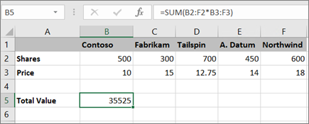
The formula first multiplies the shares (cells B2 – F2) by their prices (cells B3 – F3), and then adds those results to create a grand total of 35,525. This is an example of a single-cell array formula because the formula lives in just one cell.

Press Enter (if you have a current Microsoft 365 Subscription); otherwise press Ctrl+Shift+Enter.

When you press Ctrl+Shift+Enter, Excel automatically inserts the formula between (a pair of opening and closing braces).

To calculate multiple results by using an array formula, enter the array into a range of cells that has the exact same number of rows and columns that you’ll use in the array arguments.

Select the range of cells in which you want to enter the array formula.

Enter the formula that you want to use.

Array formulas use standard formula syntax. They all begin with an equal sign (=), and you can use any of the built-in Excel functions in your array formulas.

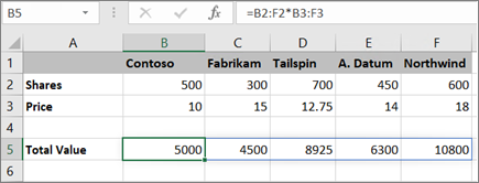
In the following example, the formula multiples shares by price in each column, and the formula lives in the selected cells in row 5.

Press Enter (if you have a current Microsoft 365 Subscription); otherwise press Ctrl+Shift+Enter.

When you press Ctrl+Shift+Enter, Excel automatically inserts the formula between (a pair of opening and closing braces).

If you need to include new data in your array formula, see Expand an array formula. You can also try:

Delete an array formula (you press Ctrl+Shift+Enter there, too)

Name an array constant (they can make constants easier to use)

Источник

VBA — Create an array from another array

I would like to know how to do this, if possible. I have defined the arrayC(26) as:

Based on the value of another cell, if it has a value of 3 I want to go from A to C. If it has a value of 5, I want to go from A to E. And so on.

Let us assume it goes from A to C. So, I want that in arrayCont(j) I have the following values «A,B,C». Then I will go to Cells(8,»C») to check if it is equal to the value in the arrayCont(j). If so, I want to remove that value from the arrayCont(j). For instance, consider that Cells(8,»C») = «B». Then my arrayCont(j) will be «A,C». How can I do this?

The code I have created is:

Thank you in advance.

1 Answer 1

First, in order to add all the letters inside your brackets to elements in an array, the array need to be dynamic ( Dim arrayC As. ) , and not static ( Dim arrayC(26) As. ). Also, either you use Split , or you need to add » before and after each element inside your brackets.

Second, in order to find if the value in «C8» is found inside the copied array ( arrayCont ) , which is Redim up to i (=3), we use the Application.Match to find the index of the matching element inside the array. If there is a «match» then we remove that element from the array.

Third I am using a Sub called «DeleteElementAt» which removes a certain element from an array, depeneds on the index of the array you want to remove.

My Code (Tested)

Sub DeleteElementAt Code

Источник

Guidelines and examples of array formulas

An array formula is a formula that can perform multiple calculations on one or more items in an array. You can think of an array as a row or column of values, or a combination of rows and columns of values. Array formulas can return either multiple results, or a single result.

Beginning with the September 2018 update for Microsoft 365, any formula that can return multiple results will automatically spill them either down, or across into neighboring cells. This change in behavior is also accompanied by several new dynamic array functions. Dynamic array formulas, whether they’re using existing functions or the dynamic array functions, only need to be input into a single cell, then confirmed by pressing Enter. Earlier, legacy array formulas require first selecting the entire output range, then confirming the formula with Ctrl+Shift+Enter. They’re commonly referred to as CSE formulas.

You can use array formulas to perform complex tasks, such as:

Quickly create sample datasets.

Count the number of characters contained in a range of cells.

Sum only numbers that meet certain conditions, such as the lowest values in a range, or numbers that fall between an upper and lower boundary.

Sum every Nth value in a range of values.

The following examples show you how to create multi-cell and single-cell array formulas. Where possible, we’ve included examples with some of the dynamic array functions, as well as existing array formulas entered as both dynamic and legacy arrays.

Download our examples

This exercise shows you how to use multi-cell and single-cell array formulas to calculate a set of sales figures. The first set of steps uses a multi-cell formula to calculate a set of subtotals. The second set uses a single-cell formula to calculate a grand total.

Multi-cell array formula

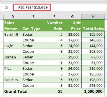
Here we’re calculating Total Sales of coupes and sedans for each salesperson by entering =F10:F19*G10:G19 in cell H10.

When you press Enter, you’ll see the results spill down to cells H10:H19. Notice that the spill range is highlighted with a border when you select any cell within the spill range. You might also notice that the formulas in cells H10:H19 are grayed out. They’re just there for reference, so if you want to adjust the formula, you’ll need to select cell H10, where the master formula lives.

Single-cell array formula

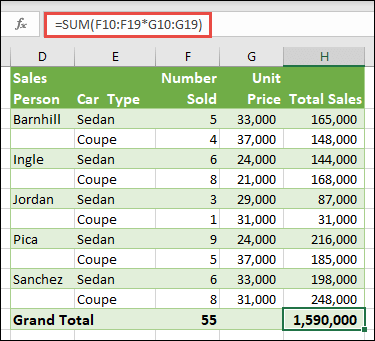
In cell H20 of the example workbook, type or copy and paste =SUM(F10:F19*G10:G19), and then press Enter.

In this case, Excel multiplies the values in the array (the cell range F10 through G19), and then uses the SUM function to add the totals together. The result is a grand total of $1,590,000 in sales.

This example shows how powerful this type of formula can be. For example, suppose you have 1,000 rows of data. You can sum part or all of that data by creating an array formula in a single cell instead of dragging the formula down through the 1,000 rows. Also, notice that the single-cell formula in cell H20 is completely independent of the multi-cell formula (the formula in cells H10 through H19). This is another advantage of using array formulas — flexibility. You could change the other formulas in column H without affecting the formula in H20. It can also be good practice to have independent totals like this, as it helps validate the accuracy of your results.

Dynamic array formulas also offer these advantages:

Consistency If you click any of the cells from H10 downward, you see the same formula. That consistency can help ensure greater accuracy.

Safety You can’t overwrite a component of a multi-cell array formula. For example, click cell H11 and press Delete. Excel won’t change the array’s output. To change it, you need to select the top-left cell in the array, or cell H10.

Smaller file sizes You can often use a single array formula instead of several intermediate formulas. For example, the car sales example uses one array formula to calculate the results in column E. If you had used standard formulas such as =F10*G10, F11*G11, F12*G12, etc., you would have used 11 different formulas to calculate the same results. That’s not a big deal, but what if you had thousands of rows to total? Then it can make a big difference.

Efficiency Array functions can be an efficient way to build complex formulas. The array formula =SUM(F10:F19*G10:G19) is the same as this: =SUM(F10*G10,F11*G11,F12*G12,F13*G13,F14*G14,F15*G15,F16*G16,F17*G17,F18*G18,F19*G19).

Spilling Dynamic array formulas will automatically spill into the output range. If your source data is in an Excel table, then your dynamic array formulas will automatically resize as you add or remove data.

#SPILL! error Dynamic arrays introduced the #SPILL! error, which indicates that the intended spill range is blocked for some reason. When you resolve the blockage, the formula will automatically spill.

Array constants are a component of array formulas. You create array constants by entering a list of items and then manually surrounding the list with braces (< >), like this:

If you separate the items by using commas, you create a horizontal array (a row). If you separate the items by using semicolons, you create a vertical array (a column). To create a two-dimensional array, you delimit the items in each row with commas, and delimit each row with semicolons.

The following procedures will give you some practice in creating horizontal, vertical, and two-dimensional constants. We’ll show examples using the SEQUENCE function to automatically generate array constants, as well as manually entered array constants.

Create a horizontal constant

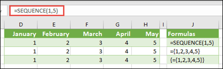
Use the workbook from the previous examples, or create a new workbook. Select any empty cell and enter =SEQUENCE(1,5). The SEQUENCE function builds a 1 row by 5 column array the same as = . The following result is displayed:

Create a vertical constant

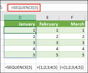
Select any blank cell with room beneath it, and enter =SEQUENCE(5), or = . The following result is displayed:

Create a two-dimensional constant

Select any blank cell with room to the right and beneath it, and enter =SEQUENCE(3,4). You see the following result:

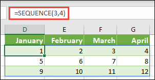
You can also enter: or =<1,2,3,4;5,6,7,8;9,10,11,12>, but you’ll want to pay attention to where you put semi-colons versus commas.

As you can see, the SEQUENCE option offers significant advantages over manually entering your array constant values. Primarily, it saves you time, but it can also help reduce errors from manual entry. It’s also easier to read, especially as the semi-colons can be hard to distinguish from the comma separators.

Here’s an example that uses array constants as part of a bigger formula. In the sample workbook, go to the Constant in a formula worksheet, or create a new worksheet.

In cell D9, we entered =SEQUENCE(1,5,3,1), but you could also enter 3, 4, 5, 6, and 7 in cells A9:H9. There’s nothing special about that particular number selection, we just chose something other than 1-5 for differentiation.

In cell E11, enter =SUM(D9:H9*SEQUENCE(1,5)), or =SUM(D9:H9*<1,2,3,4,5>). The formulas return 85.

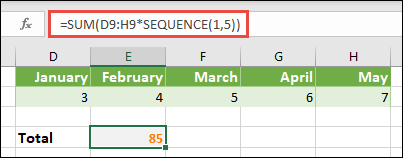
The SEQUENCE function builds the equivalent of the array constant <1,2,3,4,5>. Because Excel performs operations on expressions enclosed in parentheses first, the next two elements that come into play are the cell values in D9:H9, and the multiplication operator (*). At this point, the formula multiplies the values in the stored array by the corresponding values in the constant. It’s the equivalent of:

Finally, the SUM function adds the values, and returns 85.

To avoid using the stored array and keep the operation entirely in memory, you can replace it with another array constant:

Elements that you can use in array constants

Array constants can contain numbers, text, logical values (such as TRUE and FALSE), and error values such as #N/A. You can use numbers in integer, decimal, and scientific formats. If you include text, you need to surround it with quotation marks («text”).

Array constants can’t contain additional arrays, formulas, or functions. In other words, they can contain only text or numbers that are separated by commas or semicolons. Excel displays a warning message when you enter a formula such as <1,2,A1:D4>or <1,2,SUM(Q2:Z8)>. Also, numeric values can’t contain percent signs, dollar signs, commas, or parentheses.

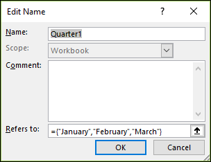
One of the best ways to use array constants is to name them. Named constants can be much easier to use, and they can hide some of the complexity of your array formulas from others. To name an array constant and use it in a formula, do the following:

Go to Formulas > Defined Names > Define Name. In the Name box, type Quarter1. In the Refers to box, enter the following constant (remember to type the braces manually):

The dialog box should now look like this:

Defined Names > Name Manager > New» loading=»lazy»>

Click OK, then select any row with three blank cells, and enter =Quarter1.

The following result is displayed:

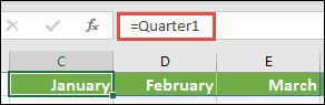
If you want the results to spill vertically instead of horizontally, you can use =TRANSPOSE(Quarter1).

If you want to display a list of 12 months, like you might use when building a financial statement, you can base one off the current year with the SEQUENCE function. The neat thing about this function is that even though only the month is displaying, there is a valid date behind it that you can use in other calculations. You’ll find these examples on the Named array constant and Quick sample dataset worksheets in the example workbook.

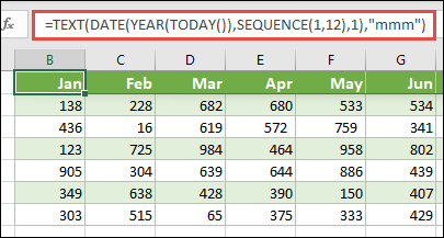
This uses the DATE function to create a date based on the current year, SEQUENCE creates an array constant from 1 to 12 for January through December, then the TEXT function converts the display format to «mmm» (Jan, Feb, Mar, etc.). If you wanted to display the full month name, such as January, you’d use «mmmm».

When you use a named constant as an array formula, remember to enter the equal sign, as in =Quarter1, not just Quarter1. If you don’t, Excel interprets the array as a string of text and your formula won’t work as expected. Finally, keep in mind that you can use combinations of functions, text and numbers. It all depends on how creative you want to get.

The following examples demonstrate a few of the ways in which you can put array constants to use in array formulas. Some of the examples use the TRANSPOSE function to convert rows to columns and vice versa.

Multiple each item in an array

You can also divide with ( /), add with ( +), and subtract with ( —).

Square the items in an array

Find the square root of squared items in an array

Transpose a one-dimensional row

Enter =TRANSPOSE(SEQUENCE(1,5)), or =TRANSPOSE(<1,2,3,4,5>)

Even though you entered a horizontal array constant, the TRANSPOSE function converts the array constant into a column.

Transpose a one-dimensional column

Enter =TRANSPOSE(SEQUENCE(5,1)), or =TRANSPOSE(<1;2;3;4;5>)

Even though you entered a vertical array constant, the TRANSPOSE function converts the constant into a row.

Transpose a two-dimensional constant

The TRANSPOSE function converts each row into a series of columns.

This section provides examples of basic array formulas.

Create an array from existing values

The following example explains how to use array formulas to create a new array from an existing array.

Enter =SEQUENCE(3,6,10,10), or =

Be sure to type < (opening brace) before you type 10, and >(closing brace) after you type 180, because you’re creating an array of numbers.

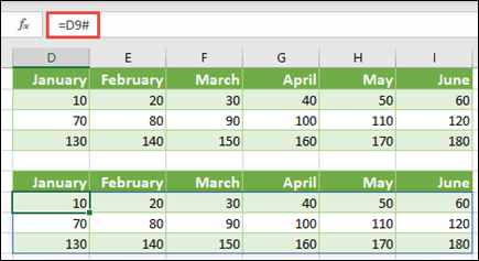
Next, enter =D9#, or =D9:I11 in a blank cell. A 3 x 6 array of cells appears with the same values you see in D9:D11. The # sign is called the spilled range operator, and it’s Excel’s way of referencing the entire array range instead of having to type it out.

Create an array constant from existing values

You can take the results of a spilled array formula and convert that into its component parts. Select cell D9, then press F2 to switch to edit mode. Next, press F9 to convert the cell references to values, which Excel then converts into an array constant. When you press Enter, the formula, =D9#, should now be =<10,20,30;40,50,60;70,80,90>.

Count characters in a range of cells

The following example shows you how to count the number of characters in a range of cells. This includes spaces.

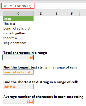
In this case, the LEN function returns the length of each text string in each of the cells in the range. The SUM function then adds those values together and displays the result (66). If you wanted to get average number of characters, you could use:

Contents of longest cell in range C9:C13

This formula works only when a data range contains a single column of cells.

Let’s take a closer look at the formula, starting from the inner elements and working outward. The LEN function returns the length of each of the items in the cell range D2:D6. The MAX function calculates the largest value among those items, which corresponds to the longest text string, which is in cell D3.

Here’s where things get a little complex. The MATCH function calculates the offset (the relative position) of the cell that contains the longest text string. To do that, it requires three arguments: a lookup value, a lookup array, and a match type. The MATCH function searches the lookup array for the specified lookup value. In this case, the lookup value is the longest text string:

and that string resides in this array:

The match type argument in this case is 0. The match type can be a 1, 0, or -1 value.

1 — returns the largest value that is less than or equal to the lookup val

0 — returns the first value exactly equal to the lookup value

-1 — returns the smallest value that is greater than or equal to the specified lookup value

If you omit a match type, Excel assumes 1.

Finally, the INDEX function takes these arguments: an array, and a row and column number within that array. The cell range C9:C13 provides the array, the MATCH function provides the cell address, and the final argument (1) specifies that the value comes from the first column in the array.

If you wanted to get the contents of the smallest text string, you would replace MAX in the above example with MIN.

Find the n smallest values in a range

This example shows how to find the three smallest values in a range of cells, where an array of sample data in cells B9:B18has been created with: =INT(RANDARRAY(10,1)*100). Note that RANDARRAY is a volatile function, so you’ll get a new set of random numbers each time Excel calculates.

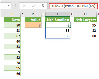
Enter =SMALL(B9#,SEQUENCE(D9), =SMALL(B9:B18,<1;2;3>)

This formula uses an array constant to evaluate the SMALL function three times and return the smallest 3 members in the array that’s contained in cells B9:B18, where 3 is a variable value in cell D9. To find more values, you can increase the value in the SEQUENCE function, or add more arguments to the constant. You can also use additional functions with this formula, such as SUM or AVERAGE. For example:

Find the n largest values in a range

To find the largest values in a range, you can replace the SMALL function with the LARGE function. In addition, the following example uses the ROW and INDIRECT functions.

Enter =LARGE(B9#,ROW(INDIRECT(«1:3»))), or =LARGE(B9:B18,ROW(INDIRECT(«1:3»)))

At this point, it may help to know a bit about the ROW and INDIRECT functions. You can use the ROW function to create an array of consecutive integers. For example, select an empty and enter:

The formula creates a column of 10 consecutive integers. To see a potential problem, insert a row above the range that contains the array formula (that is, above row 1). Excel adjusts the row references, and the formula now generates integers from 2 to 11. To fix that problem, you add the INDIRECT function to the formula:

The INDIRECT function uses text strings as its arguments (which is why the range 1:10 is surrounded by quotation marks). Excel does not adjust text values when you insert rows or otherwise move the array formula. As a result, the ROW function always generates the array of integers that you want. You could just as easily use SEQUENCE:

Let’s examine the formula that you used earlier — =LARGE(B9#,ROW(INDIRECT(«1:3»))) — starting from the inner parentheses and working outward: The INDIRECT function returns a set of text values, in this case the values 1 through 3. The ROW function in turn generates a three-cell column array. The LARGE function uses the values in the cell range B9:B18, and it is evaluated three times, once for each reference returned by the ROW function. If you want to find more values, you add a greater cell range to the INDIRECT function. Finally, as with the SMALL examples, you can use this formula with other functions, such as SUM and AVERAGE.

Sum a range that contains error values

The SUM function in Excel does not work when you try to sum a range that contains an error value, such as #VALUE! or #N/A. This example shows you how to sum the values in a range named Data that contains errors:

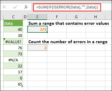
The formula creates a new array that contains the original values minus any error values. Starting from the inner functions and working outward, the ISERROR function searches the cell range (Data) for errors. The IF function returns a specific value if a condition you specify evaluates to TRUE and another value if it evaluates to FALSE. In this case, it returns empty strings («») for all error values because they evaluate to TRUE, and it returns the remaining values from the range (Data) because they evaluate to FALSE, meaning that they don’t contain error values. The SUM function then calculates the total for the filtered array.

Count the number of error values in a range

This example is like the previous formula, but it returns the number of error values in a range named Data instead of filtering them out:

This formula creates an array that contains the value 1 for the cells that contain errors and the value 0 for the cells that don’t contain errors. You can simplify the formula and achieve the same result by removing the third argument for the IF function, like this:

If you don’t specify the argument, the IF function returns FALSE if a cell does not contain an error value. You can simplify the formula even more:

This version works because TRUE*1=1 and FALSE*1=0.

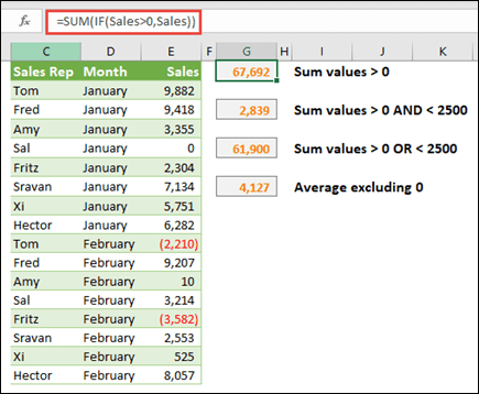
You might need to sum values based on conditions.

0,Sales)) will sum all values greater than 0 in a range called Sales.» loading=»lazy»>

For example, this array formula sums just the positive integers in a range named Sales, which represents cells E9:E24 in the example above:

The IF function creates an array of positive and false values. The SUM function essentially ignores the false values because 0+0=0. The cell range that you use in this formula can consist of any number of rows and columns.

You can also sum values that meet more than one condition. For example, this array formula calculates values greater than 0 AND less than 2500:

=SUM((Sales>0)*(Sales OR less than 2500:

The IF function creates an array of values that do not equal 0 and then passes those values to the AVERAGE function.

This array formula compares the values in two ranges of cells named MyData and YourData and returns the number of differences between the two. If the contents of the two ranges are identical, the formula returns 0. To use this formula, the cell ranges need to be the same size and of the same dimension. For example, if MyData is a range of 3 rows by 5 columns, YourData must also be 3 rows by 5 columns:

The formula creates a new array of the same size as the ranges that you are comparing. The IF function fills the array with the value 0 and the value 1 (0 for mismatches and 1 for identical cells). The SUM function then returns the sum of the values in the array.

You can simplify the formula like this:

Like the formula that counts error values in a range, this formula works because TRUE*1=1, and FALSE*1=0.

This array formula returns the row number of the maximum value in a single-column range named Data:

The IF function creates a new array that corresponds to the range named Data. If a corresponding cell contains the maximum value in the range, the array contains the row number. Otherwise, the array contains an empty string («»). The MIN function uses the new array as its second argument and returns the smallest value, which corresponds to the row number of the maximum value in Data. If the range named Data contains identical maximum values, the formula returns the row of the first value.

If you want to return the actual cell address of a maximum value, use this formula:

You’ll find similar examples in the sample workbook on the Differences between datasets worksheet.

Multi-cell array formula

Copy the entire table below and paste it into cell A1 in a blank worksheet.

Formula (Grand Total)

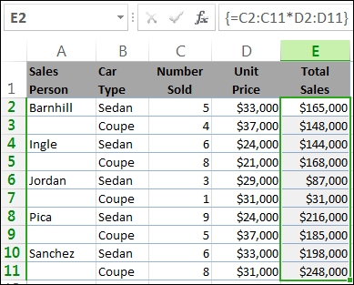
To see Total Sales of coupes and sedans for each salesperson, select cells E2:E11, enter the formula =C2:C11*D2:D11, and then press Ctrl+Shift+Enter.

To see the Grand Total of all sales, select cell F11, enter the formula =SUM(C2:C11*D2:D11), and then press Ctrl+Shift+Enter.

When you press Ctrl+Shift+Enter, Excel surrounds the formula with braces ( ) and inserts an instance of the formula in each cell of the selected range. This happens very quickly, so what you see in column E is the total sales amount for each car type for each salesperson. If you select E2, then select E3, E4, and so on, you’ll see that the same formula is shown: .

Create a single-cell array formula

In cell D13 of the workbook, type the following formula, and then press Ctrl+Shift+Enter:

In this case, Excel multiplies the values in the array (the cell range C2 through D11) and then uses the SUM function to add the totals together. The result is a grand total of $1,590,000 in sales. This example shows how powerful this type of formula can be. For example, suppose you have 1,000 rows of data. You can sum part or all of that data by creating an array formula in a single cell instead of dragging the formula down through the 1,000 rows.

Also, notice that the single-cell formula in cell D13 is completely independent of the multi-cell formula (the formula in cells E2 through E11). This is another advantage of using array formulas — flexibility. You could change the formulas in column E or delete that column altogether, without affecting the formula in D13.

Array formulas also offer these advantages:

Consistency If you click any of the cells from E2 downward, you see the same formula. That consistency can help ensure greater accuracy.

Safety You cannot overwrite a component of a multi-cell array formula. For example, click cell E3 and press Delete. You have to either select the entire range of cells (E2 through E11) and change the formula for the entire array, or leave the array as is. As an added safety measure, you have to press Ctrl+Shift+Enter to confirm any change to the formula.

Smaller file sizes You can often use a single array formula instead of several intermediate formulas. For example, the workbook uses one array formula to calculate the results in column E. If you had used standard formulas (such as =C2*D2, C3*D3, C4*D4…), you would have used 11 different formulas to calculate the same results.

In general, array formulas use standard formula syntax. They all begin with an equal (=) sign, and you can use most of the built-in Excel functions in your array formulas. The key difference is that when using an array formula, you press Ctrl+Shift+Enter to enter your formula. When you do this, Excel surrounds your array formula with braces — if you type the braces manually, your formula will be converted to a text string, and it won’t work.

Array functions can be an efficient way to build complex formulas. The array formula =SUM(C2:C11*D2:D11) is the same as this: =SUM(C2*D2,C3*D3,C4*D4,C5*D5,C6*D6,C7*D7,C8*D8,C9*D9,C10*D10,C11*D11).

Important: Press Ctrl+Shift+Enter whenever you need to enter an array formula. This applies to both single-cell and multi-cell formulas.

Whenever you work with multi-cell formulas, also remember:

Select the range of cells to hold your results before you enter the formula. You did this when you created the multi-cell array formula when you selected cells E2 through E11.

You can’t change the contents of an individual cell in an array formula. To try this, select cell E3 in the workbook and press Delete. Excel displays a message that tells you that you can’t change part of an array.

You can move or delete an entire array formula, but you can’t move or delete part of it. In other words, to shrink an array formula, you first delete the existing formula and then start over.

To delete an array formula, select the entire formula range (for example, E2:E11), then press Delete.

You can’t insert blank cells into, or delete cells from a multi-cell array formula.

At times, you may need to expand an array formula. Select the first cell in existing array range, and continue until you’ve selected the entire range that you want to extend the formula to. Press F2 to edit the formula, then press CTRL+SHIFT+ENTER to confirm the formula once you’ve adjusted the formula range. The key is to select the entire range, starting with the top-left cell in the array. The top-left cell is the one that gets edited.

Array formulas are great, but they can have some disadvantages:

You may occasionally forget to press Ctrl+Shift+Enter. It can happen to even the most experienced Excel users. Remember to press this key combination whenever you enter or edit an array formula.

Other users of your workbook might not understand your formulas. In practice, array formulas are generally not explained in a worksheet. Therefore, if other people need to modify your workbooks, you should either avoid array formulas or make sure those people know about any array formulas and understand how to change them, if they need to.

Depending on the processing speed and memory of your computer, large array formulas can slow down calculations.

Array constants are a component of array formulas. You create array constants by entering a list of items and then manually surrounding the list with braces ( ), like this:

By now, you know you need to press Ctrl+Shift+Enter when you create array formulas. Because array constants are a component of array formulas, you surround the constants with braces by manually typing them. You then use Ctrl+Shift+Enter to enter the entire formula.

Here’s an array in a single row: <1,2,3,4>. Here’s an array in a single column: <1;2;3;4>. And here’s an array of two rows and four columns: <1,2,3,4;5,6,7,8>. In the two row array, the first row is 1, 2, 3, and 4, and the second row is 5, 6, 7, and 8. A single semicolon separates the two rows, between 4 and 5.

As with array formulas, you can use array constants with most of the built-in functions that Excel provides. The following sections explain how to create each kind of constant and how to use these constants with functions in Excel.

The following procedures will give you some practice in creating horizontal, vertical, and two-dimensional constants.

Create a horizontal constant

In a blank worksheet, select cells A1 through E1.

In the formula bar, enter the following formula, and then press Ctrl+Shift+Enter:

In this case, you should type the opening and closing braces ( ), and Excel will add the second set for you.

The following result is displayed.

Create a vertical constant

In your workbook, select a column of five cells.

In the formula bar, enter the following formula, and then press Ctrl+Shift+Enter:

The following result is displayed.

Create a two-dimensional constant

In your workbook, select a block of cells four columns wide by three rows high.

In the formula bar, enter the following formula, and then press Ctrl+Shift+Enter:

You see the following result:

Use constants in formulas

Here is a simple example that uses constants:

In the sample workbook, create a new worksheet.

In cell A1, type 3, and then type 4 in B1, 5 in C1, 6 in D1, and 7 in E1.

In cell A3, type the following formula, and then press Ctrl+Shift+Enter:

Notice that Excel surrounds the constant with another set of braces, because you entered it as an array formula.

The value 85 appears in cell A3.

The next section explains how the formula works.

The formula you just used contains several parts.

4. Array constant

The last element inside the parentheses is the array constant: . Remember that Excel does not surround array constants with braces; you actually type them. Also remember that after you add a constant to an array formula, you press Ctrl+Shift+Enter to enter the formula.

Because Excel performs operations on expressions enclosed in parentheses first, the next two elements that come into play are the values stored in the workbook (A1:E1) and the operator. At this point, the formula multiplies the values in the stored array by the corresponding values in the constant. It’s the equivalent of:

Finally, the SUM function adds the values, and the sum 85 appears in cell A3.

To avoid using the stored array and to just keep the operation entirely in memory, replace the stored array with another array constant:

To try this, copy the function, select a blank cell in your workbook, paste the formula into the formula bar, and then press Ctrl+Shift+Enter. You’ll see the same result as you did in the earlier exercise that used the array formula:

Array constants can contain numbers, text, logical values (such as TRUE and FALSE), and error values ( such as #N/A). You can use numbers in the integer, decimal, and scientific formats. If you include text, you need to surround the text with quotation marks ( «).

One of the best way to use array constants is to name them. Named constants can be much easier to use, and they can hide some of the complexity of your array formulas from others. To name an array constant and use it in a formula, do the following:

On the Formulas tab, in the Defined Names group, click Define Name.
The Define Name dialog box appears.

In the Name box, type Quarter1.

In the Refers to box, enter the following constant (remember to type the braces manually):

The contents of the dialog box now looks like this:

Click OK, and then select a row of three blank cells.

Type the following formula, and then press Ctrl+Shift+Enter.

The following result is displayed.

When you use a named constant as an array formula, remember to enter the equal sign. If you don’t, Excel interprets the array as a string of text and your formula won’t work as expected. Finally, keep in mind that you can use combinations of text and numbers.

Look for the following problems when your array constants don’t work:

Some elements might not be separated with the proper character. If you omit a comma or semicolon, or if you put one in the wrong place, the array constant might not be created correctly, or you might see a warning message.

You might have selected a range of cells that doesn’t match the number of elements in your constant. For example, if you select a column of six cells for use with a five-cell constant, the #N/A error value appears in the empty cell. Conversely, if you select too few cells, Excel omits the values that don’t have a corresponding cell.

Multiply each item in an array

Create a new worksheet, and then select a block of empty cells four columns wide by three rows high.

Type the following formula, and then press Ctrl+Shift+Enter:

Square the items in an array

Select a block of empty cells four columns wide by three rows high.

Type the following array formula, and then press Ctrl+Shift+Enter:

Alternatively, enter this array formula, which uses the caret operator ( ^):

Transpose a one-dimensional row

Select a column of five blank cells.

Type the following formula, and then press Ctrl+Shift+Enter:

Even though you entered a horizontal array constant, the TRANSPOSE function converts the array constant into a column.

Transpose a one-dimensional column

Select a row of five blank cells.

Enter the following formula, and then press Ctrl+Shift+Enter:

Even though you entered a vertical array constant, the TRANSPOSE function converts the constant into a row.

Transpose a two-dimensional constant

Select a block of cells three columns wide by four rows high.

Enter the following constant, and then press Ctrl+Shift+Enter:

The TRANSPOSE function converts each row into a series of columns.

This section provides examples of basic array formulas.

Create arrays and array constants from existing values

The following example explains how to use array formulas to create links between ranges of cells in different worksheets. It also shows you how to create an array constant from the same set of values.

Create an array from existing values

On a worksheet in Excel, select cells C8:E10, and enter this formula:

Be sure to type <(opening brace) before you type 10, and > (closing brace) after you type 90, because you’re creating an array of numbers.

Press Ctrl+Shift+Enter, which enters this array of numbers in the cell range C8:E10 by using an array formula. On your worksheet, C8 through E10 should look like this:

Select the cell range C1 through E3.

Enter the following formula in the formula bar, and then press Ctrl+Shift+Enter:

A 3×3 array of cells appears in cells C1 through E3 with the same values you see in C8 through E10.

Create an array constant from existing values

With cells C1:C3 selected, press F2 to switch to edit mode.

Press F9 to convert the cell references to values. Excel converts the values into an array constant. The formula should now be = .

Press Ctrl+Shift+Enter to enter the array constant as an array formula.

Count characters in a range of cells

The following example shows you how to count the number of characters, including spaces, in a range of cells.

Copy this entire table and paste into a worksheet in cell A1.

bunch of cells that

Total characters in A2:A6

Contents of longest cell (A3)

Select cell A8, and then press Ctrl+Shift+Enter to see the total number of characters in cells A2:A6 (66).

Select cell A10, and then press Ctrl+Shift+Enter to see the contents of the longest of cells A2:A6 (cell A3).

The following formula is used in cell A8 counts the total number of characters (66) in cells A2 through A6.

In this case, the LEN function returns the length of each text string in each of the cells in the range. The SUM function then adds those values together and displays the result (66).

Find the n smallest values in a range

This example shows how to find the three smallest values in a range of cells.

Enter some random numbers in cells A1:A11.

Select cells C1 through C3. This set of cells will hold the results returned by the array formula.

Enter the following formula, and then press Ctrl+Shift+Enter:

This formula uses an array constant to evaluate the SMALL function three times and return the smallest (1), second smallest (2), and third smallest (3) members in the array that is contained in cells A1:A10 To find more values, you add more arguments to the constant. You can also use additional functions with this formula, such as SUM or AVERAGE. For example:

Find the n largest values in a range

To find the largest values in a range, you can replace the SMALL function with the LARGE function. In addition, the following example uses the ROW and INDIRECT functions.

Select cells D1 through D3.

In the formula bar, enter this formula, and then press Ctrl+Shift+Enter:

At this point, it may help to know a bit about the ROW and INDIRECT functions. You can use the ROW function to create an array of consecutive integers. For example, select an empty column of 10 cells in your practice workbook, enter this array formula, and then press Ctrl+Shift+Enter:

The formula creates a column of 10 consecutive integers. To see a potential problem, insert a row above the range that contains the array formula (that is, above row 1). Excel adjusts the row references, and the formula generates integers from 2 to 11. To fix that problem, you add the INDIRECT function to the formula:

The INDIRECT function uses text strings as its arguments (which is why the range 1:10 is surrounded by double quotation marks). Excel does not adjust text values when you insert rows or otherwise move the array formula. As a result, the ROW function always generates the array of integers that you want.

Let’s take a look at the formula that you used earlier — =LARGE(A5:A14,ROW(INDIRECT(«1:3»))) — starting from the inner parentheses and working outward: The INDIRECT function returns a set of text values, in this case the values 1 through 3. The ROW function in turn generates a three-cell columnar array. The LARGE function uses the values in the cell range A5:A14, and it is evaluated three times, once for each reference returned by the ROW function. The values 3200, 2700, and 2000 are returned to the three-cell columnar array. If you want to find more values, you add a greater cell range to the INDIRECT function.

As with earlier examples, you can use this formula with other functions, such as SUM and AVERAGE.

Find the longest text string in a range of cells

Go back to the earlier text string example, enter the following formula in an empty cell, and press Ctrl+Shift+Enter:

The text «bunch of cells that» appears.

Let’s take a closer look at the formula, starting from the inner elements and working outward. The LEN function returns the length of each of the items in the cell range A2:A6. The MAX function calculates the largest value among those items, which corresponds to the longest text string, which is in cell A3.

and that string resides in this array:

The match type argument is 0. The match type can consist of a 1, 0, or -1 value. If you specify 1, MATCH returns the largest value that is less than or equal to the lookup value. If you specify 0, MATCH returns the first value exactly equal to the lookup value. If you specify -1, MATCH finds the smallest value that is greater than or equal to the specified lookup value. If you omit a match type, Excel assumes 1.

Finally, the INDEX function takes these arguments: an array, and a row and column number within that array. The cell range A2:A6 provides the array, the MATCH function provides the cell address, and the final argument ( 1) specifies that the value comes from the first column in the array.

This section provides examples of advanced array formulas.

Sum a range that contains error values

The SUM function in Excel does not work when you try to sum a range that contains an error value, such as #N/A. This example shows you how to sum the values in a range named Data that contains errors.

The formula creates a new array that contains the original values minus any error values. Starting from the inner functions and working outward, the ISERROR function searches the cell range (Data) for errors. The IF function returns a specific value if a condition you specify evaluates to TRUE and another value if it evaluates to FALSE. In this case, it returns empty strings ( «») for all error values because they evaluate to TRUE, and it returns the remaining values from the range ( Data) because they evaluate to FALSE, meaning that they don’t contain error values. The SUM function then calculates the total for the filtered array.

Count the number of error values in a range

This example is similar to the previous formula, but it returns the number of error values in a range named Data instead of filtering them out:

If you don’t specify the argument, the IF function returns FALSE if a cell does not contain an error value. You can simplify the formula even more:

This version works because TRUE*1=1 and FALSE*1=0.

Sum values based on conditions

You might need to sum values based on conditions. For example, this array formula sums just the positive integers in a range named Sales:

The IF function creates an array of positive values and false values. The SUM function essentially ignores the false values because 0+0=0. The cell range that you use in this formula can consist of any number of rows and columns.

You can also sum values that meet more than one condition. For example, this array formula calculates values greater than 0 and less than or equal to 5:

=SUM((Sales>0)*(Sales =SUM(IF((Sales 15),Sales))

The IF function finds all values smaller than 5 and greater than 15 and then passes those values to the SUM function.

You can’t use the AND and OR functions in array formulas directly because those functions return a single result, either TRUE or FALSE, and array functions require arrays of results. You can work around the problem by using the logic shown in the previous formula. In other words, you perform math operations, such as addition or multiplication, on values that meet the OR or AND condition.

Compute an average that excludes zeros

This example shows you how to remove zeros from a range when you need to average the values in that range. The formula uses a data range named Sales:

The IF function creates an array of values that do not equal 0 and then passes those values to the AVERAGE function.

Count the number of differences between two ranges of cells

This array formula compares the values in two ranges of cells named MyData and YourData and returns the number of differences between the two. If the contents of the two ranges are identical, the formula returns 0. To use this formula, the cell ranges need to be the same size and of the same dimension (for example, if MyData is a range of 3 rows by 5 columns, YourData must also be 3 rows by 5 columns):

You can simplify the formula like this:

Like the formula that counts error values in a range, this formula works because TRUE*1=1, and FALSE*1=0.

Find the location of the maximum value in a range

This array formula returns the row number of the maximum value in a single-column range named Data:

The IF function creates a new array that corresponds to the range named Data. If a corresponding cell contains the maximum value in the range, the array contains the row number. Otherwise, the array contains an empty string ( «»). The MIN function uses the new array as its second argument and returns the smallest value, which corresponds to the row number of the maximum value in Data. If the range named Data contains identical maximum values, the formula returns the row of the first value.

If you want to return the actual cell address of a maximum value, use this formula:

Acknowledgement

Parts of this article were based on a series of Excel Power User columns written by Colin Wilcox, and adapted from chapters 14 and 15 of Excel 2002 Formulas, a book written by John Walkenbach, a former Excel MVP.

Need more help?

You can always ask an expert in the Excel Tech Community or get support in the Answers community.

Источник

First, in order to add all the letters inside your brackets to elements in an array, the array need to be dynamic (Dim arrayC As...) , and not static (Dim arrayC(26) As...). Also, either you use Split, or you need to add " before and after each element inside your brackets.

Second, in order to find if the value in «C8» is found inside the copied array (arrayCont) , which is Redim up to i (=3), we use the Application.Match to find the index of the matching element inside the array. If there is a «match» then we remove that element from the array.

Third I am using a Sub called «DeleteElementAt» which removes a certain element from an array, depeneds on the index of the array you want to remove.

My Code (Tested)

Option Explicit

Sub SubArrayfromArray()

Dim arrayC As Variant
Dim i As Integer 'Position in the arrayC(26)
Dim arrayCont As Variant

' this is the way to put all the strings inside the brackets in an array (type Variant) in one line of code
arrayC = Array("A", "B", "C", "D", "E", "F", "G", "H", "I", "J", "K", "L", "M", "N", "O", "P", "Q", "R", "S", "T", "U", "V", "W", "X", "Y", "Z")
i = 3 ' i is the value of another worksheet cell

' copy original dynamic array to destination dynamic array
arrayCont = arrayC

' redim the copied array up to 3 (from 0 to 2)
ReDim Preserve arrayCont(0 To i - 1)

' value in Range C8  >> if "B" was found inside the arrayCont >> remove it from the array
If Not IsError(Application.Match(Range("C8").Value, arrayCont, 0)) Then
    Call DeleteElementAt(Application.Match(Range("C8").Value, arrayCont, 0) - 1, arrayCont)
End If
' for debug only
'For i = LBound(arrayCont) To UBound(arrayCont)
'    MsgBox "Array element " & i & " Value is " & arrayCont(i)
'Next i

' Edit 1: place arrayCont result in Cells(9, 3) >> Range("C9")
Range("C9").Resize(UBound(arrayCont) + 1, 1).Value = Application.Transpose(arrayCont)

End Sub

Sub DeleteElementAt Code

Public Sub DeleteElementAt(ByVal ArrIndex As Integer, ByRef myArr As Variant)

' this sub removes a certain element from the array, then it shrinks the size of the array by 1    
Dim i As Integer

' move all element back one position
For i = ArrIndex + 1 To UBound(myArr)
    myArr(i - 1) = myArr(i)
Next

' shrink the array by one, removing the last one
ReDim Preserve myArr(UBound(myArr) - 1)

End Sub

Источник

Excel для Microsoft 365 Excel для Microsoft 365 для Mac Excel для Интернета Еще…Меньше

Возвращает вычисляемый массив строк и столбцов указанного размера путем применения функции ЛЯМБДА.

Синтаксис

=MAKEARRAY(строки, столбцы, лямбда(строка, столбец))

Аргументы и параметры функции MAKEARRAY:

строки. Количество строк в массиве. Должно быть больше нуля.
столбцы. Количество столбцов в массиве. Должно быть больше нуля.
лямбда. Функция ЛЯМБДА, вызываемая для создания массива. ЛЯМБДА принимает два параметра:
- строка. Индекс строки массива.
- столбец. Индекс столбца массива.

Ошибки

При указании недопустимой функции ЛЯМБДА или неверного количества параметров возвращается ошибка #ЗНАЧ! с названием «Неверные параметры».

Если аргументам строка или столбец присвоено значение < 1 или не число, возвращается ошибка #ЗНАЧ! .

Примеры

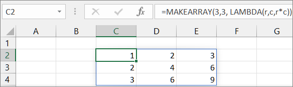
Пример 1. Создание двухмерного массива, представляющего простую таблицу умножения

В ячейку C2 скопируйте следующую формулу:

=MAKEARRAY(3, 3, LAMBDA(r,c, r*c))

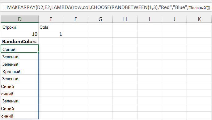
Пример 2. Создание случайного списка значений

Введите пример данных в ячейки D1:E3, а затем скопируйте формулу в ячейку D4:

=MAKEARRAY(D2,E2,LAMBDA(row,col,CHOOSE(RANDBETWEEN(1,3),»Red»,»Blue»,»Green»)))

См. также

Функция LAMBDA

Функция MAP

Функция REDUCE

Функция SCAN

Функция BYCOL

Функция BYROW

Функция ISOMITTED

Нужна дополнительная помощь?

Источник

This post provides an in-depth look at the VBA array which is a very important part of the Excel VBA programming language. It covers everything you need to know about the VBA array.

We will start by seeing what exactly is the VBA Array is and why you need it.

Below you will see a quick reference guide to using the VBA Array. Refer to it anytime you need a quick reminder of the VBA Array syntax.

The rest of the post provides the most complete guide you will find on the VBA array.

A Quick Guide to the VBA Array

Task	Static Array	Dynamic Array
Declare	Dim arr(0 To 5) As Long	Dim arr() As Long Dim arr As Variant
Set Size	See Declare above	ReDim arr(0 To 5)As Variant
Get Size(number of items)	See ArraySize function below.	See ArraySize function below.
Increase size (keep existing data)	Dynamic Only	ReDim Preserve arr(0 To 6)
Set values	arr(1) = 22	arr(1) = 22
Receive values	total = arr(1)	total = arr(1)
First position	LBound(arr)	LBound(arr)
Last position	Ubound(arr)	Ubound(arr)
Read all items(1D)	For i = LBound(arr) To UBound(arr) Next i Or For i = LBound(arr,1) To UBound(arr,1) Next i	For i = LBound(arr) To UBound(arr) Next i Or For i = LBound(arr,1) To UBound(arr,1) Next i
Read all items(2D)	For i = LBound(arr,1) To UBound(arr,1) For j = LBound(arr,2) To UBound(arr,2) Next j Next i	For i = LBound(arr,1) To UBound(arr,1) For j = LBound(arr,2) To UBound(arr,2) Next j Next i
Read all items	Dim item As Variant For Each item In arr Next item	Dim item As Variant For Each item In arr Next item
Pass to Sub	Sub MySub(ByRef arr() As String)	Sub MySub(ByRef arr() As String)
Return from Function	Function GetArray() As Long() Dim arr(0 To 5) As Long GetArray = arr End Function	Function GetArray() As Long() Dim arr() As Long GetArray = arr End Function
Receive from Function	Dynamic only	Dim arr() As Long Arr = GetArray()
Erase array	Erase arr *Resets all values to default	Erase arr *Deletes array
String to array	Dynamic only	Dim arr As Variant arr = Split(«James:Earl:Jones»,»:»)
Array to string	Dim sName As String sName = Join(arr, «:»)	Dim sName As String sName = Join(arr, «:»)
Fill with values	Dynamic only	Dim arr As Variant arr = Array(«John», «Hazel», «Fred»)
Range to Array	Dynamic only	Dim arr As Variant arr = Range(«A1:D2»)
Array to Range	Same as dynamic	Dim arr As Variant Range(«A5:D6») = arr

Download the Source Code and Data

Please click on the button below to get the fully documented source code for this article.

What is the VBA Array and Why do You Need It?

A VBA array is a type of variable. It is used to store lists of data of the same type. An example would be storing a list of countries or a list of weekly totals.

In VBA a normal variable can store only one value at a time.

In the following example we use a variable to store the marks of a student:

' Can only store 1 value at a time
Dim Student1 As Long
Student1 = 55

If we wish to store the marks of another student then we need to create a second variable.

In the following example, we have the marks of five students:

Student Marks

We are going to read these marks and write them to the Immediate Window.

Note: The function Debug.Print writes values to the Immediate Window. To view this window select View->Immediate Window from the menu( Shortcut is Ctrl + G)

As you can see in the following example we are writing the same code five times – once for each student:

' https://excelmacromastery.com/
Public Sub StudentMarks()

    ' Get the worksheet called "Marks"
    Dim sh As Worksheet
    Set sh = ThisWorkbook.Worksheets("Marks")
    
    ' Declare variable for each student
    Dim Student1 As Long
    Dim Student2 As Long
    Dim Student3 As Long
    Dim Student4 As Long
    Dim Student5 As Long

    ' Read student marks from cell
    Student1 = sh.Range("C" & 3).Value
    Student2 = sh.Range("C" & 4).Value
    Student3 = sh.Range("C" & 5).Value
    Student4 = sh.Range("C" & 6).Value
    Student5 = sh.Range("C" & 7).Value

    ' Print student marks
    Debug.Print "Students Marks"
    Debug.Print Student1
    Debug.Print Student2
    Debug.Print Student3
    Debug.Print Student4
    Debug.Print Student5

End Sub

The following is the output from the example:

Output

The problem with using one variable per student is that you need to add code for each student. Therefore if you had a thousand students in the above example you would need three thousand lines of code!

Luckily we have arrays to make our life easier. Arrays allow us to store a list of data items in one structure.

The following code shows the above student example using an array:

' ExcelMacroMastery.com
' https://excelmacromastery.com/excel-vba-array/
' Author: Paul Kelly
' Description: Reads marks to an Array and write
' the array to the Immediate Window(Ctrl + G)
' TO RUN: Click in the sub and press F5
Public Sub StudentMarksArr()

    ' Get the worksheet called "Marks"
    Dim sh As Worksheet
    Set sh = ThisWorkbook.Worksheets("Marks")

    ' Declare an array to hold marks for 5 students
    Dim Students(1 To 5) As Long

    ' Read student marks from cells C3:C7 into array
    ' Offset counts rows from cell C2.
    ' e.g. i=1 is C2 plus 1 row which is C3
    '      i=2 is C2 plus 2 rows which is C4
    Dim i As Long
    For i = 1 To 5
        Students(i) = sh.Range("C2").Offset(i).Value
    Next i

    ' Print student marks from the array to the Immediate Window
    Debug.Print "Students Marks"
    For i = LBound(Students) To UBound(Students)
        Debug.Print Students(i)
    Next i

End Sub

The advantage of this code is that it will work for any number of students. If we have to change this code to deal with 1000 students we only need to change the (1 To 5) to (1 To 1000) in the declaration. In the prior example we would need to add approximately five thousand lines of code.

Let’s have a quick comparison of variables and arrays. First we compare the declaration:

        ' Variable
        Dim Student As Long
        Dim Country As String

        ' Array
        Dim Students(1 To 3) As Long
        Dim Countries(1 To 3) As String

Next we compare assigning a value:

        ' assign value to variable
        Student1 = .Cells(1, 1) 

        ' assign value to first item in array
        Students(1) = .Cells(1, 1)

Finally we look at writing the values:

        ' Print variable value
        Debug.Print Student1

        ' Print value of first student in array
        Debug.Print Students(1)

As you can see, using variables and arrays is quite similar.

The fact that arrays use an index(also called a subscript) to access each item is important. It means we can easily access all the items in an array using a For Loop.

Now that you have some background on why arrays are useful let’s go through them step by step.

Two Types of VBA Arrays

There are two types of VBA arrays:

Static – an array of fixed length.
Dynamic(not to be confused with the Excel Dynamic Array) – an array where the length is set at run time.

The difference between these types is mostly in how they are created. Accessing values in both array types is exactly the same. In the following sections we will cover both of these types.

VBA Array Initialization

A static array is initialized as follows:

' https://excelmacromastery.com/
Public Sub DecArrayStatic()

    ' Create array with locations 0,1,2,3
    Dim arrMarks1(0 To 3) As Long

    ' Defaults as 0 to 3 i.e. locations 0,1,2,3
    Dim arrMarks2(3) As Long

    ' Create array with locations 1,2,3,4,5
    Dim arrMarks3(1 To 5) As Long

    ' Create array with locations 2,3,4 ' This is rarely used
    Dim arrMarks4(2 To 4) As Long

End Sub

An Array of 0 to 3

As you can see the length is specified when you declare a static array. The problem with this is that you can never be sure in advance the length you need. Each time you run the Macro you may have different length requirements.

If you do not use all the array locations then the resources are being wasted. So if you need more locations you can use ReDim but this is essentially creating a new static array.

The dynamic array does not have such problems. You do not specify the length when you declare it. Therefore you can then grow and shrink as required:

' https://excelmacromastery.com/
Public Sub DecArrayDynamic()

    ' Declare  dynamic array
    Dim arrMarks() As Long

    ' Set the length of the array when you are ready
    ReDim arrMarks(0 To 5)

End Sub

The dynamic array is not allocated until you use the ReDim statement. The advantage is you can wait until you know the number of items before setting the array length. With a static array you have to state the length upfront.

To give an example. Imagine you were reading worksheets of student marks. With a dynamic array you can count the students on the worksheet and set an array to that length. With a static array you must set the length to the largest possible number of students.

Assigning Values to VBA Array

To assign values to an array you use the number of the location. You assign the value for both array types the same way:

' https://excelmacromastery.com/
Public Sub AssignValue()

    ' Declare  array with locations 0,1,2,3
    Dim arrMarks(0 To 3) As Long

    ' Set the value of position 0
    arrMarks(0) = 5

    ' Set the value of position 3
    arrMarks(3) = 46

    ' This is an error as there is no location 4
    arrMarks(4) = 99

End Sub

The array with values assigned

The number of the location is called the subscript or index. The last line in the example will give a “Subscript out of Range” error as there is no location 4 in the array example.

VBA Array Length

There is no native function for getting the number of items in an array. I created the ArrayLength function below to return the number of items in any array no matter how many dimensions:

' https://excelmacromastery.com/
Function ArrayLength(arr As Variant) As Long

    On Error Goto eh
    
    ' Loop is used for multidimensional arrays. The Loop will terminate when a
    ' "Subscript out of Range" error occurs i.e. there are no more dimensions.
    Dim i As Long, length As Long
    length = 1
    
    ' Loop until no more dimensions
    Do While True
        i = i + 1
        ' If the array has no items then this line will throw an error
        Length = Length * (UBound(arr, i) - LBound(arr, i) + 1)
        ' Set ArrayLength here to avoid returing 1 for an empty array
        ArrayLength = Length
    Loop

Done:
    Exit Function
eh:
    If Err.Number = 13 Then ' Type Mismatch Error
        Err.Raise vbObjectError, "ArrayLength" _
            , "The argument passed to the ArrayLength function is not an array."
    End If
End Function

You can use it like this:

' Name: TEST_ArrayLength
' Author: Paul Kelly, ExcelMacroMastery.com
' Description: Tests the ArrayLength functions and writes
'              the results to the Immediate Window(Ctrl + G)
Sub TEST_ArrayLength()
    
    ' 0 items
    Dim arr1() As Long
    Debug.Print ArrayLength(arr1)
    
    ' 10 items
    Dim arr2(0 To 9) As Long
    Debug.Print ArrayLength(arr2)
    
    ' 18 items
    Dim arr3(0 To 5, 1 To 3) As Long
    Debug.Print ArrayLength(arr3)
    
    ' Option base 0: 144 items
    ' Option base 1: 50 items
    Dim arr4(1, 5, 5, 0 To 1) As Long
    Debug.Print ArrayLength(arr4)
    
End Sub

Using the Array and Split function

You can use the Array function to populate an array with a list of items. You must declare the array as a type Variant. The following code shows you how to use this function.

    Dim arr1 As Variant
    arr1 = Array("Orange", "Peach","Pear")

    Dim arr2 As Variant
    arr2 = Array(5, 6, 7, 8, 12)

Contents of arr1 after using the Array function

The array created by the Array Function will start at index zero unless you use Option Base 1 at the top of your module. Then it will start at index one. In programming, it is generally considered poor practice to have your actual data in the code. However, sometimes it is useful when you need to test some code quickly.

The Split function is used to split a string into an array based on a delimiter. A delimiter is a character such as a comma or space that separates the items.

The following code will split the string into an array of four elements:

    Dim s As String
    s = "Red,Yellow,Green,Blue"

    Dim arr() As String
    arr = Split(s, ",")

The array after using Split

The Split function is normally used when you read from a comma-separated file or another source that provides a list of items separated by the same character.

Using Loops With the VBA Array

Using a For Loop allows quick access to all items in an array. This is where the power of using arrays becomes apparent. We can read arrays with ten values or ten thousand values using the same few lines of code. There are two functions in VBA called LBound and UBound. These functions return the smallest and largest subscript in an array. In an array arrMarks(0 to 3) the LBound will return 0 and UBound will return 3.

The following example assigns random numbers to an array using a loop. It then prints out these numbers using a second loop.

' https://excelmacromastery.com/
Public Sub ArrayLoops()

    ' Declare  array
    Dim arrMarks(0 To 5) As Long

    ' Fill the array with random numbers
    Dim i As Long
    For i = LBound(arrMarks) To UBound(arrMarks)
        arrMarks(i) = 5 * Rnd
    Next i

    ' Print out the values in the array
    Debug.Print "Location", "Value"
    For i = LBound(arrMarks) To UBound(arrMarks)
        Debug.Print i, arrMarks(i)
    Next i

End Sub

The functions LBound and UBound are very useful. Using them means our loops will work correctly with any array length. The real benefit is that if the length of the array changes we do not have to change the code for printing the values. A loop will work for an array of any length as long as you use these functions.

Using the For Each Loop with the VBA Array

You can use the For Each loop with arrays. The important thing to keep in mind is that it is Read-Only. This means that you cannot change the value in the array.

In the following code the value of mark changes but it does not change the value in the array.

    For Each mark In arrMarks
        ' Will not change the array value
        mark = 5 * Rnd
    Next mark

The For Each is loop is fine to use for reading an array. It is neater to write especially for a Two-Dimensional array as we will see.

    Dim mark As Variant
    For Each mark In arrMarks
        Debug.Print mark
    Next mark

Using Erase with the VBA Array

The Erase function can be used on arrays but performs differently depending on the array type.

For a static Array the Erase function resets all the values to the default. If the array is made up of long integers(i.e type Long) then all the values are set to zero. If the array is of strings then all the strings are set to “” and so on.

For a Dynamic Array the Erase function DeAllocates memory. That is, it deletes the array. If you want to use it again you must use ReDim to Allocate memory.

Let’s have a look an example for the static array. This example is the same as the ArrayLoops example in the last section with one difference – we use Erase after setting the values. When the value are printed out they will all be zero:

' https://excelmacromastery.com/
Public Sub EraseStatic()

    ' Declare  array
    Dim arrMarks(0 To 3) As Long

    ' Fill the array with random numbers
    Dim i As Long
    For i = LBound(arrMarks) To UBound(arrMarks)
        arrMarks(i) = 5 * Rnd
    Next i

    ' ALL VALUES SET TO ZERO
    Erase arrMarks

    ' Print out the values - there are all now zero
    Debug.Print "Location", "Value"
    For i = LBound(arrMarks) To UBound(arrMarks)
        Debug.Print i, arrMarks(i)
    Next i

End Sub

We will now try the same example with a dynamic. After we use Erase all the locations in the array have been deleted. We need to use ReDim if we wish to use the array again.

If we try to access members of this array we will get a “Subscript out of Range” error:

' https://excelmacromastery.com/
Public Sub EraseDynamic()

    ' Declare  array
    Dim arrMarks() As Long
    ReDim arrMarks(0 To 3)

    ' Fill the array with random numbers
    Dim i As Long
    For i = LBound(arrMarks) To UBound(arrMarks)
        arrMarks(i) = 5 * Rnd
    Next i

    ' arrMarks is now deallocated. No locations exist.
    Erase arrMarks

End Sub

Increasing the length of the VBA Array

If we use ReDim on an existing array, then the array and its contents will be deleted.

In the following example, the second ReDim statement will create a completely new array. The original array and its contents will be deleted.

' https://excelmacromastery.com/
Sub UsingRedim()

    Dim arr() As String
    
    ' Set array to be slots 0 to 2
    ReDim arr(0 To 2)
    arr(0) = "Apple"
    
    ' Array with apple is now deleted
    ReDim arr(0 To 3)

End Sub

If we want to extend the length of an array without losing the contents, we can use the Preserve keyword.

When we use Redim Preserve the new array must start at the same starting dimension e.g.

We cannot Preserve from (0 to 2) to (1 to 3) or to (2 to 10) as they are different starting dimensions.

In the following code we create an array using ReDim and then fill the array with types of fruit.

We then use Preserve to extend the length of the array so we don’t lose the original contents:

' https://excelmacromastery.com/
Sub UsingRedimPreserve()

    Dim arr() As String
    
    ' Set array to be slots 0 to 1
    ReDim arr(0 To 2)
    arr(0) = "Apple"
    arr(1) = "Orange"
    arr(2) = "Pear"
    
    ' Reset the length and keep original contents
    ReDim Preserve arr(0 To 5)

End Sub

You can see from the screenshots below, that the original contents of the array have been “Preserved”.

Before ReDim Preserve

After ReDim Preserve

Word of Caution: In most cases, you shouldn’t need to resize an array like we have done in this section. If you are resizing an array multiple times then you may want to consider using a Collection.

Using Preserve with Two-Dimensional Arrays

Preserve only works with the upper bound of an array.

For example, if you have a two-dimensional array you can only preserve the second dimension as this example shows:

' https://excelmacromastery.com/
Sub Preserve2D()

    Dim arr() As Long
    
    ' Set the starting length
    ReDim arr(1 To 2, 1 To 5)
    
    ' Change the length of the upper dimension
    ReDim Preserve arr(1 To 2, 1 To 10)

End Sub

If we try to use Preserve on a lower bound we will get the “Subscript out of range” error.

In the following code we use Preserve on the first dimension. Running this code will give the “Subscript out of range” error:

' https://excelmacromastery.com/
Sub Preserve2DError()

    Dim arr() As Long
    
    ' Set the starting length
    ReDim arr(1 To 2, 1 To 5)
    
    ' "Subscript out of Range" error
    ReDim Preserve arr(1 To 5, 1 To 5)

End Sub

When we read from a range to an array, it automatically creates a two-dimensional array, even if we have only one column.

The same Preserve rules apply. We can only use Preserve on the upper bound as this example shows:

' https://excelmacromastery.com/
Sub Preserve2DRange()

    Dim arr As Variant
    
    ' Assign a range to an array
    arr = Sheet1.Range("A1:A5").Value
    
    ' Preserve will work on the upper bound only
    ReDim Preserve arr(1 To 5, 1 To 7)

End Sub

Sorting the VBA Array

There is no function in VBA for sorting an array. We can sort the worksheet cells but this could be slow if there is a lot of data.

The QuickSort function below can be used to sort an array.

' https://excelmacromastery.com/
Sub QuickSort(arr As Variant, first As Long, last As Long)
  
  Dim vCentreVal As Variant, vTemp As Variant
  
  Dim lTempLow As Long
  Dim lTempHi As Long
  lTempLow = first
  lTempHi = last
  
  vCentreVal = arr((first + last)  2)
  Do While lTempLow <= lTempHi
  
    Do While arr(lTempLow) < vCentreVal And lTempLow < last
      lTempLow = lTempLow + 1
    Loop
    
    Do While vCentreVal < arr(lTempHi) And lTempHi > first
      lTempHi = lTempHi - 1
    Loop
    
    If lTempLow <= lTempHi Then
    
        ' Swap values
        vTemp = arr(lTempLow)

        arr(lTempLow) = arr(lTempHi)
        arr(lTempHi) = vTemp
      
        ' Move to next positions
        lTempLow = lTempLow + 1
        lTempHi = lTempHi - 1
      
    End If
    
  Loop
  
  If first < lTempHi Then QuickSort arr, first, lTempHi
  If lTempLow < last Then QuickSort arr, lTempLow, last
  
End Sub

You can use this function like this:

' https://excelmacromastery.com/
Sub TestSort()

    ' Create temp array
    Dim arr() As Variant
    arr = Array("Banana", "Melon", "Peach", "Plum", "Apple")
  
    ' Sort array
    QuickSort arr, LBound(arr), UBound(arr)

    ' Print arr to Immediate Window(Ctrl + G)
    Dim i As Long
    For i = LBound(arr) To UBound(arr)
        Debug.Print arr(i)
    Next i

End Sub

Passing the VBA Array to a Sub

Sometimes you will need to pass an array to a procedure. You declare the parameter using parenthesis similar to how you declare a dynamic array.

Passing to the procedure using ByRef means you are passing a reference of the array. So if you change the array in the procedure it will be changed when you return.

Note: When you use an array as a parameter it cannot use ByVal, it must use ByRef. You can pass the array using ByVal making the parameter a variant.

' https://excelmacromastery.com/
' Passes array to a Function
Public Sub PassToProc()
    Dim arr(0 To 5) As String
    ' Pass the array to function
    UseArray arr
End Sub

Public Function UseArray(ByRef arr() As String)
    ' Use array
    Debug.Print UBound(arr)
End Function

Returning the VBA Array from a Function

It is important to keep the following in mind. If you want to change an existing array in a procedure then you should pass it as a parameter using ByRef(see last section). You do not need to return the array from the procedure.

The main reason for returning an array is when you use the procedure to create a new one. In this case you assign the return array to an array in the caller. This array cannot be already allocated. In other words you must use a dynamic array that has not been allocated.

The following examples show this

' https://excelmacromastery.com/
Public Sub TestArray()

    ' Declare dynamic array - not allocated
    Dim arr() As String
    ' Return new array
    arr = GetArray

End Sub

Public Function GetArray() As String()

    ' Create and allocate new array
    Dim arr(0 To 5) As String
    ' Return array
    GetArray = arr

End Function

Using a Two-Dimensional VBA Array

The arrays we have been looking at so far have been one-dimensional arrays. This means the arrays are one list of items.

A two-dimensional array is essentially a list of lists. If you think of a single spreadsheet row as a single dimension then more than one column is two dimensional. In fact a spreadsheet is the equivalent of a two-dimensional array. It has two dimensions – rows and columns.

One small thing to note is that Excel treats a one-dimensional array as a row if you write it to a spreadsheet. In other words, the array arr(1 to 5) is equivalent to arr(1 to 1, 1 to 5) when writing values to the spreadsheet.

The following image shows two groups of data. The first is a one-dimensional layout and the second is two dimensional.

To access an item in the first set of data(1 dimensional) all you need to do is give the row e.g. 1,2, 3 or 4.

For the second set of data (two-dimensional), you need to give the row AND the column. So you can think of 1 dimensional being multiple columns and one row and two-dimensional as being multiple rows and multiple columns.

Note: It is possible to have more than two dimensions in an array. It is rarely required. If you are solving a problem using a 3+ dimensional array then there probably is a better way to do it.

You declare a two-dimensional array as follows:

Dim ArrayMarks(0 To 2,0 To 3) As Long

The following example creates a random value for each item in the array and the prints the values to the Immediate Window:

' https://excelmacromastery.com/
Public Sub TwoDimArray()

    ' Declare a two dimensional array
    Dim arrMarks(0 To 3, 0 To 2) As String

    ' Fill the array with text made up of i and j values
    Dim i As Long, j As Long
    For i = LBound(arrMarks) To UBound(arrMarks)
        For j = LBound(arrMarks, 2) To UBound(arrMarks, 2)
            arrMarks(i, j) = CStr(i) & ":" & CStr(j)
        Next j
    Next i

    ' Print the values in the array to the Immediate Window
    Debug.Print "i", "j", "Value"
    For i = LBound(arrMarks) To UBound(arrMarks)
        For j = LBound(arrMarks, 2) To UBound(arrMarks, 2)
            Debug.Print i, j, arrMarks(i, j)
        Next j
    Next i

End Sub

You can see that we use a second For loop inside the first loop to access all the items.

The output of the example looks like this:

How this Macro works is as follows:

Enters the i loop
i is set to 0
Entersj loop
j is set to 0
j is set to 1
j is set to 2
Exit j loop
i is set to 1
j is set to 0
j is set to 1
j is set to 2
And so on until i=3 and j=2

You may notice that LBound and UBound have a second argument with the value 2. This specifies that it is the upper or lower bound of the second dimension. That is the start and end location for j. The default value 1 which is why we do not need to specify it for the i loop.

Using the For Each Loop

Using a For Each is neater to use when reading from an array.

Let’s take the code from above that writes out the two-dimensional array

    ' Using For loop needs two loops
    Debug.Print "i", "j", "Value"
    For i = LBound(arrMarks) To UBound(arrMarks)
        For j = LBound(arrMarks, 2) To UBound(arrMarks, 2)
            Debug.Print i, j, arrMarks(i, j)
        Next j
    Next i

Now let’s rewrite it using a For each loop. You can see we only need one loop and so it is much easier to write:

    ' Using For Each requires only one loop
    Debug.Print "Value"
    Dim mark As Variant
    For Each mark In arrMarks
        Debug.Print mark
    Next mark

Using the For Each loop gives us the array in one order only – from LBound to UBound. Most of the time this is all you need.

Reading from a Range to the VBA Array

If you have read my previous post on Cells and Ranges then you will know that VBA has an extremely efficient way of reading from a Range of Cells to an Array and vice versa

' https://excelmacromastery.com/
Public Sub ReadToArray()

    ' Declare dynamic array
    Dim StudentMarks As Variant

    ' Read values into array from first row
    StudentMarks = Range("A1:Z1").Value

    ' Write the values back to the third row
    Range("A3:Z3").Value = StudentMarks

End Sub

The dynamic array created in this example will be a two dimensional array. As you can see we can read from an entire range of cells to an array in just one line.

The next example will read the sample student data below from C3:E6 of Sheet1 and print them to the Immediate Window:

' https://excelmacromastery.com/
Public Sub ReadAndDisplay()

    ' Get Range
    Dim rg As Range
    Set rg = ThisWorkbook.Worksheets("Sheet1").Range("C3:E6")

    ' Create dynamic array
    Dim StudentMarks As Variant

    ' Read values into array from sheet1
    StudentMarks = rg.Value

    ' Print the array values
    Debug.Print "i", "j", "Value"
    Dim i As Long, j As Long
    For i = LBound(StudentMarks) To UBound(StudentMarks)
        For j = LBound(StudentMarks, 2) To UBound(StudentMarks, 2)
            Debug.Print i, j, StudentMarks(i, j)
        Next j
    Next i

End Sub

Sample Student data

Output from sample data

As you can see the first dimension(accessed using i) of the array is a row and the second is a column. To demonstrate this take a look at the value 44 in E4 of the sample data. This value is in row 2 column 3 of our data. You can see that 44 is stored in the array at StudentMarks(2,3).

You can see more about using arrays with ranges in this YouTube video

How To Make Your Macros Run at Super Speed

If your macros are running very slow then you may find this section very helpful. Especially if you are dealing with large amounts of data. The following is a very well-kept secret in VBA

Updating values in arrays is exponentially faster than updating values in cells.

In the last section, you saw how we can easily read from a group of cells to an array and vice versa. If we are updating a lot of values then we can do the following:

1. Copy the data from the cells to an array.
2. Change the data in the array.
3. Copy the updated data from the array back to the cells.

For example, the following code would be much faster than the code below it:

' https://excelmacromastery.com/
Public Sub ReadToArray()

    ' Read values into array from first row
    Dim StudentMarks  As Variant
    StudentMarks = Range("A1:Z20000").Value

    Dim i As Long
    For i = LBound(StudentMarks) To UBound(StudentMarks)
        ' Update marks here
        StudentMarks(i, 1) = StudentMarks(i, 1) * 2
        '...
    Next i

    ' Write the new values back to the worksheet
    Range("A1:Z20000").Value = StudentMarks

End Sub

' https://excelmacromastery.com/
Sub UsingCellsToUpdate()
    
    Dim c As Variant
    For Each c In Range("A1:Z20000")
        c.Value = ' Update values here
    Next c
    
End Sub

Assigning from one set of cells to another is also much faster than using Copy and Paste:

' Assigning - this is faster
Range("A1:A10").Value = Range("B1:B10").Value

' Copy Paste - this is slower
Range("B1:B1").Copy Destination:=Range("A1:A10")

The following comments are from two readers who used arrays to speed up their macros

“A couple of my projects have gone from almost impossible and long to run into almost too easy and a reduction in time to run from 10:1.” – Dane

“One report I did took nearly 3 hours to run when accessing the cells directly — 5 minutes with arrays” – Jim

You can see more about the speed of Arrays compared to other methods in this YouTube video.

To see a comparison between Find, Match and Arrays it is worth checking out this post by Charles Williams.

Conclusion

The following is a summary of the main points of this post

Arrays are an efficient way of storing a list of items of the same type.
You can access an array item directly using the number of the location which is known as the subscript or index.
The common error “Subscript out of Range” is caused by accessing a location that does not exist.
There are two types of arrays: Static and Dynamic.
Static is used when the length of the array is always the same.
Dynamic arrays allow you to determine the length of an array at run time.
LBound and UBound provide a safe way of find the smallest and largest subscripts of the array.
The basic array is one dimensional. You can also have multidimensional arrays.
You can only pass an array to a procedure using ByRef. You do this like this: ByRef arr() as long.
You can return an array from a function but the array, it is assigned to, must not be currently allocated.
A worksheet with its rows and columns is essentially a two-dimensional array.
You can read directly from a worksheet range into a two-dimensional array in just one line of code.
You can also write from a two-dimensional array to a range in just one line of code.

What’s Next?

Free VBA Tutorial If you are new to VBA or you want to sharpen your existing VBA skills then why not try The Ultimate VBA Tutorial.

Related Training: Get full access to the Excel VBA training webinars.

(NOTE: Planning to build or manage a VBA Application? Learn how to build 10 Excel VBA applications from scratch.)

Источник

The MAKEARRAY function returns a array with specified rows and columns, based on a custom LAMBDA calculation. MAKEARRAY can be used to create arrays with variable dimensions where the values in the array are calculated.

The MAKEARRAY function takes three arguments: rows, columns, and lambda. Rows is the number of columns to create, and columns is the number or columns to create. Lambda is the calculation to use when creating values in the array. The total number of values in the array returned by MAKEARRAY will equal rows * columns.

LAMBDA structure

The MAKEARRAY uses the LAMBDA function to apply the formula required to calculate array values. The structure of the LAMBDA used by MAKEARRAY is:

LAMBDA(r,c,calculation)

where r represents the row count, and c represents the column count originally passed into MAKEARRAY, and calculation is the formula needed to create the values in the final array.

Note: to generate an array with sequential values, see the SEQUENCE function.

Examples

In the formula below, MAKEARRAY is used to create an array with 2 rows and 3 columns, populated with the result multiplying rows by columns:

=MAKEARRAY(2,3,LAMBDA(r,c,r*c)) // returns {1,2,3;2,4,6}

The result is a 2 x 3 array with six values {1,2,3;2,4,6}.

The calculation can be hardcoded. Below are examples of the same formula, with calculation hardcoded as zero and «x»:

=MAKEARRAY(2,3,LAMBDA(r,c,0)) // returns {0,0,0;0,0,0}
=MAKEARRAY(2,3,LAMBDA(r,c,"x")) // returns {"x","x","x";"x","x","x"}

Random values

MAKEARRAY can be used to generate random values. In the formula below. The CHAR function is used with the RANDBETWEEN function to generate random uppercase letters A-Z:

=MAKEARRAY(2,3,LAMBDA(r,c,CHAR(RANDBETWEEN(65,90))))

The result is a 2 x 3 array like: {«D»,»Q»,»F»;»V»,»C»,»T»}.

Источник

Create an array formula

VBA — Create an array from another array

1 Answer 1

Guidelines and examples of array formulas

Download our examples

Acknowledgement

Need more help?

Синтаксис

Ошибки

Примеры

См. также

Нужна дополнительная помощь?

Related Links for the VBA Array

A Quick Guide to the VBA Array

Download the Source Code and Data

What is the VBA Array and Why do You Need It?

Two Types of VBA Arrays

VBA Array Initialization

Assigning Values to VBA Array

VBA Array Length

Using the Array and Split function

Using Loops With the VBA Array

Using the For Each Loop with the VBA Array

Using Erase with the VBA Array

Increasing the length of the VBA Array

Using Preserve with Two-Dimensional Arrays

Sorting the VBA Array

Passing the VBA Array to a Sub

Returning the VBA Array from a Function

Using a Two-Dimensional VBA Array

Using the For Each Loop

Reading from a Range to the VBA Array

How To Make Your Macros Run at Super Speed

Conclusion

What’s Next?

LAMBDA structure

Examples

Random values