
You have probably used color coding in your Excel data or seen it in a workbook you had to use.
It’s a popular way to visualize your data!
While colored cells are a great way to highlight data to quickly grab someone’s attention, they are not a great way to store data.
Unfortunately, a lot of users will color a cell to indicate some value instead of creating another data point with the value.
For example, they might color a cell green to indicate an item is approved instead of creating another data point with the text Approved.
This causes a lot of problems when you actually need to find out how many items were approved. Excel doesn’t offer a built-in way to count colored cells.
In this post, I’ll show you 6 ways to find and count any colored cells in your data.
Use the Find and Select Command to Count Colored Cells
Excel has a great feature that allows you to find cells based on the format. This includes any colored cells too!
You can find all the cells of a certain color, then count them.
Go to the Home tab ➜ click on the Find & Select command ➜ then choose Find from the options.
There is also a great keyboard shortcut for this. Press Ctrl + F to open the Find and Replace menu.
Click on the small down arrow in the Format button and select Choose Format From Cell.
Clicking on the main part of the Format button will open up the Find Format menu where you can select any combination of formatting to search for.
This is perfect if you know exactly what color you are searching for, but more often you will be best served by setting the format by example. Formatting could be subtilty different and this might cause you to miss finding the right data!
When you click on the small arrow inside the Format button, it will reveal more options including the ability to set the format by selecting a cell.
Once you have the format selected then click on the Find All button.
The lower part of the Find and Replace dialog box will show all the cells that were found matching the formatting and in the lower left you will find the count.
Press Ctrl + A to select all the cells and then press the Close button and you can then change the color of all these cells or change any other formatting.
If you only want to return cells in a given column, or range, this is possible. Select the range in the sheet before pressing the Find All button to limit the search to the selection.
Pros
- Easy to use.
- You can use this to search for other types of formatting and not just fill color.
- You can use this to search a selected range, the entire sheet or the entire workbook.
Cons
- This solution is not dynamic and will need to be repeated each time you want to get the count.
Use Filters and the Subtotal Function to Count Colored Cells
This method will rely on the fact that you can filter based on cell color.
First step, you will need to add filters to your data.
Select you data and go to the Data tab then choose the Filter command.
This will add a sort and filter icon to each column heading of your data and these will allow you to filter your data many different ways.
There is also a handy keyboard shortcut for adding or removing filters from your data. Select your data and press Ctrl + Shift + L on your keyboard.
Another option for adding filters is to turn your data into an Excel Table. I wrote a post all about Excel tables and the great features they come with.
You can convert your data into a table with either of these two methods.
- Select a cell inside your data ➜ go to the Insert tab ➜ click on the Table command.
- Select a cell inside your data ➜ press Ctrl + T on your keyboard.
You table should come with filters by default. If not, go to the Table tab and check the Filter Button option in the Table Style Options section.
= SUBTOTAL ( 3, Orders[Order ID] )Now you can add the above SUBTOTAL formula to count the non empty cells where Order ID is the column which contains the colored cells you would like to count.
The first argument of the SUBTOTAL function tells it to return a count while the second argument tells it what to count.
The special trick here is that the SUBTOTAL function will only count visible cells, so it will update the count based on what data it is filtered on.
This means you can filter on the colored cells and you will get a count of those colored cells!
Now you can filter your data by color.
- Click on the sort and filter toggle for the column which contains the colored cells.
- Select Filter by Color from the menu options.
- Choose the color you want to filter on.
Now the SUBTOTAL result will update and you can quickly find the count of your colored cells.
If you adjust colors, add or delete data in the table. You will need to reapply the filters as they don’t update dynamically.
Go to the Data tab and click on the Reapply button in the Sort & Filter section.
Pros
- Easy to use.
Cons
- Requires manually filtering data.
- The filters don’t update and you will need to reapply them when you change your data.
- Since the count is based on the filtering, the result can be different for each user when collaborating on the workbook.
Use the GET.CELL Macro4 Function to Count Colored Cells
Excel does have a function to get the fill color of a cell, but it is a legacy Macro 4 function.
These predate VBA and were Excel’s formula based scripting language.
While they are considered deprecated, it is still possible to use them inside the name manager.
There is a GET.CELLS Macro4 function that will return a color code based on the fill color of the cell.
You can create a relative named range that uses this by going to the Formulas tab and clicking on Define Name.
This will open up the New Name menu and you can define the reference.
Give your defined name a Name like ColorCode. This is how you will refer to it in the workbook.
= GET.CELL ( 38, Orders[@[Order ID]] )Add the above formula into the Refers to section. For this formula you data will need to be in a table named Orders with a column called Order ID, but you can change these to fit your data.
This formula will always refer to the Order ID cell in the current row to which it’s referenced.
= GET.CELL ( 38, $B3 )If your data is not inside a table, then you could use the above formula instead, where B is the column containing the fill color you want to count. This uses a fixed column and relative row reference to always refer to column B of the current row.
= ColorCodeWith the define name, you can now create another column using the above formula in your data to calculate the color code for each row.
The result will be an integer value based on the fill color of the cell in the Order ID column.
= COUNTIFS ( Orders[ColorCode], B14 )Now you can count the number or colored cells using the above COUNTIFS formula.
This formula will count cells in the ColorCode column if they have a matching code. In this example, it counts all the 10 values which correspond to the green color.
Pros
- You can calculate the fill color for each row of data and it will update dynamically as you change the data or fill color of the data.
Cons
- This method uses the Macro4 legacy functions and they may not continue to be supported my Microsoft.
- Harder to implement.
- You will need to save your workbook in the xlsm macro enabled format.
- You can’t move your referenced column if you’re using the column notation inside the named range.
- You can’t change your column name if you’re using the table notation inside the named range.
- You need to create an additional column and use a COUNTIFS function to get the count.
Use a LAMBDA Function to Count Colored Cells
This will use the same GET.CELL Macro4 function as the previous method, but you can create a custom LAMBDA function to use it inside the workbook.
The LAMBDA function is a special function that allows you to build custom functions via the name manager.
This is a new function, so it’s not generally available and you need to be on Microsoft 365 office insiders program at the time of writing this post.
Go to the Formulas tab and click on Define Name to open the New Name menu.
= LAMBDA ( cell, GET.CELL ( 38, cell ) )Give the define name a name like GETCOLORCODE and add the above formula into the Refers to section.
This will create a new GETCOLORCODE function that you can use inside the workbook. It will take one argument called cell and return the cell’s fill color code.
= GETCOLORCODE ( [@[Order ID]] )Now all you have to do is create a column to calculate the color code for each row using the above formula.
= COUNTIFS ( Orders[ColorCode], B14 )Again, you can count the number or colored cells using the the above COUNTIFS formula.
Pros
- You can build a function that calculates the color code for a given cell.
- Allows you to directly reference a cell to get the color code.
Cons
- This method uses the LAMBDA function in Excel for M365 and is currently not generally available.
- Harder to implement.
- This method uses the Macro4 legacy functions which may not be supported in the future.
- You will need to save your workbook in the xlsm macro enabled format.
- Requires creating an additional column and using a COUNTIFS function to get the count.
Use VBA to Count Colored Cells
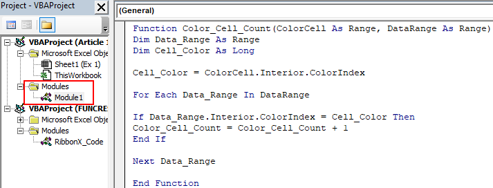
Function COLORCOUNT(CountRange As Range, FillCell As Range)
Dim FillColor As Integer
Dim Count As Integer
FillColor = FillCell.Interior.ColorIndex
For Each c In CountRange
    If c.Interior.ColorIndex = FillColor Then
        Count = Count + 1
    End If
Next c
COLORCOUNT = Count
End Function
Pros
- You can create a function that counts the colored cells in a range.
- The results will update as you edit your data or change the fill color.
- User friendly option to use once it is set up.
Cons
- Uses VBA which requires the file is saved in the xlsm format.
- Less user friendly to set up.
Use Office Scripts to Count Colored Cells
Office Scripts are the brand new method for automating tasks in Excel.
But it’s only available for Excel online and only with an enterprise plan. If you have an enterprise plan, then you’re good to go with this method!
First, you will need to set up two named cells which the code will refer to.
Select any cell and type a name like ColorCount into the name box and press Enter. This will create a named range which can be referred to in the code.
This means we can move the cell and the code will refer to its new location.
You will also need to create a Color named range for the input of the color to count.
Now you can create a new office script. Go to the Automate tab in Excel online and click on the New Script command.
function main(workbook: ExcelScript.Workbook) {
	let selectedSheet = workbook.getWorksheet("Sheet1");
	let myID = selectedSheet.getRange("Orders[Order ID]");
	let myIDCount = selectedSheet.getRange("Orders[Order ID]").getCellCount();
	let myColorCode = selectedSheet.getRange("Color").getFormat().getFill().getColor();
	let counter = 0;

	for (let i = 0; i < myIDCount; i++) {
		if (myID.getCell(i, 0).getFormat().getFill().getColor() == myColorCode ) {
			counter = counter + 1;
		}
	}

	selectedSheet.getRange("ColorCount").setValue(counter);
}
This will open up the Code Editor and you can paste in the above code and save the script.
Press the Run button and the code will execute and then populate the ColorCount named range with the count of the colored cells found in the Order ID column.
Pros
- This is the newest method and will be supported going forward.
- The script can be run from Power Automate for a no click solution.
Cons
- This method is difficult to set up.
- This requires an enterprise license and you need to use Excel online.
Conclusions
Hopefully Microsoft will one day create a standard Excel function that can return properties from a cell such as its fill color.
Until that happens, at least you have a few options available that allow you to find the count of colored cells without manually counting them.
Do you have a preferred method not listed here? Let me know in the comments!
About the Author
John is a Microsoft MVP and qualified actuary with over 15 years of experience. He has worked in a variety of industries, including insurance, ad tech, and most recently Power Platform consulting. He is a keen problem solver and has a passion for using technology to make businesses more efficient.
The COUNT function in Excel counts cells containing numbers in Excel. You cannot count colored or highlighted cells with the COUNT function. But you can follow a few workarounds to count colored cells in Excel. In this tutorial, you will learn how to count colored cells in Excel.
In excel, you can count highlighted cells using the following workarounds:
- Applying SUBTOTAL and filtering the data
- Using the COUNT and GET.CELL function
- Using VBA
Using Subtotal and Filter functions
You can count highlighted cells in Excel by subtotaling the visible cells and applying a filter based on colors.
In this example, you have the sales record for eight salespersons for the month of July. The rows containing salespersons having sales less than $7000 is highlighted in red, the other cells with the salespersons having a bonus is highlighted in green. To calculate the number of salespersons highlighted in red:
- Select the cell C10.
- Assign the formula
=SUBTOTAL(102, C2:C9). The first argument 102 counts the visible cells in the specified range.
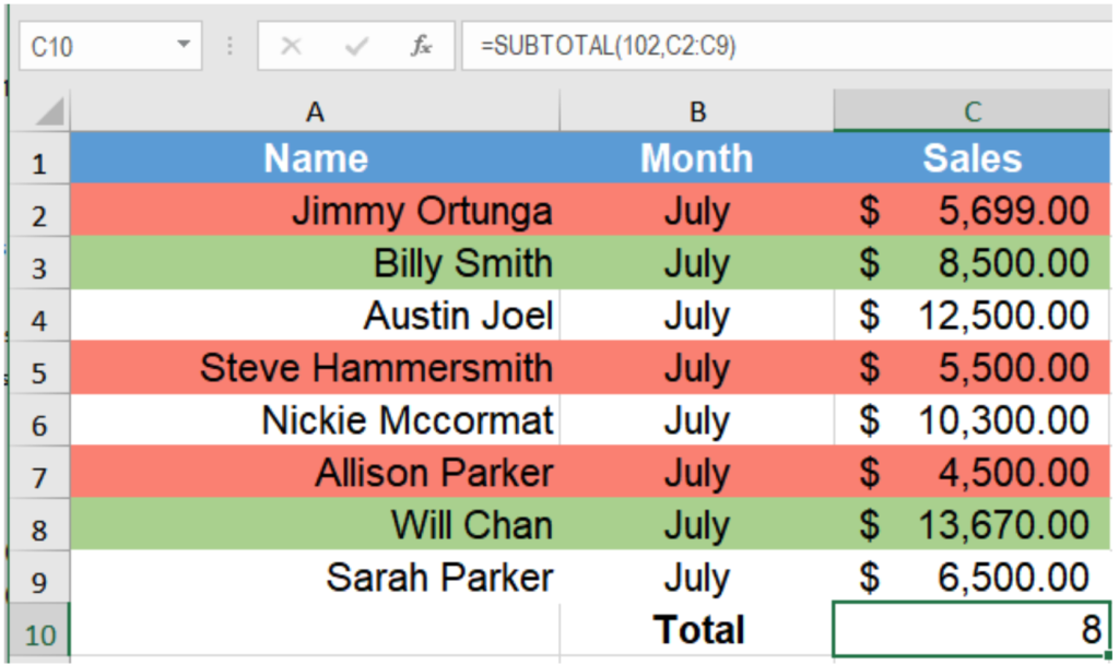
- Select cells A1:C9 by clicking on cell A1 and dragging it till C9 with your mouse.
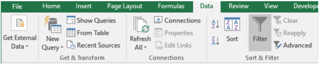
- Go to Data > Sort & Filter > Filter.
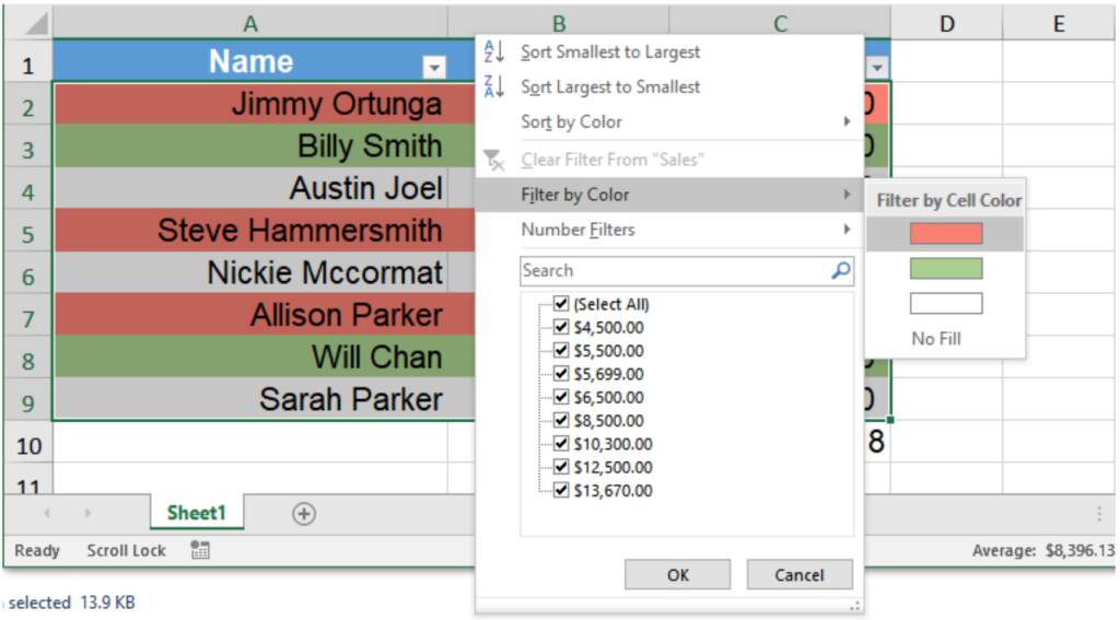
- Click on the filter drop downs in C1.
- Go to Filter by Color and select the color Red to find out the salespersons highlighted in red.
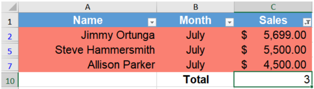
This will output change the subtotal value to x, which is the number of salespersons having sales less than $7000.
Using COUNTIF and GET.CELL functions
You can use GET.CELL with named ranges to count colored cells in Excel. GET.CELL is an old Macro4 function and does not work with regular functions. However, it still works with named ranges. To count colored cells with GET.CELL, you need to extract the color codes with GET.CELL and count them to find out the number of cells highlighted in the same color. To count cells using GET.CELL and COUNTIF:
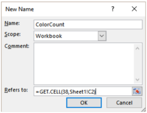
- Go to Formulas > Define Name.
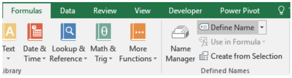
- In the dialogue box that pops up, set name as ColorCount, scope as workbook and Refers to as
=GET.CELL(38, Sheet1!C2).
- Assign the formula =ColorCount to cell D2 and drag it till D9 with your mouse.
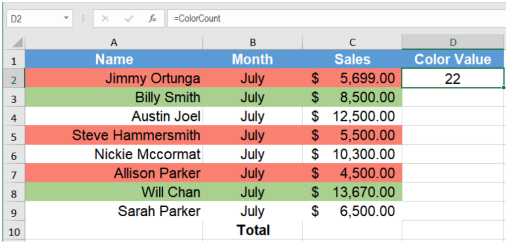
- This would return a number based on the background color. If there is no background color, Excel would return 0. Otherwise all cells with the same background color return the same number.
- From column D, look at the code for the color red. In this case it is 22.
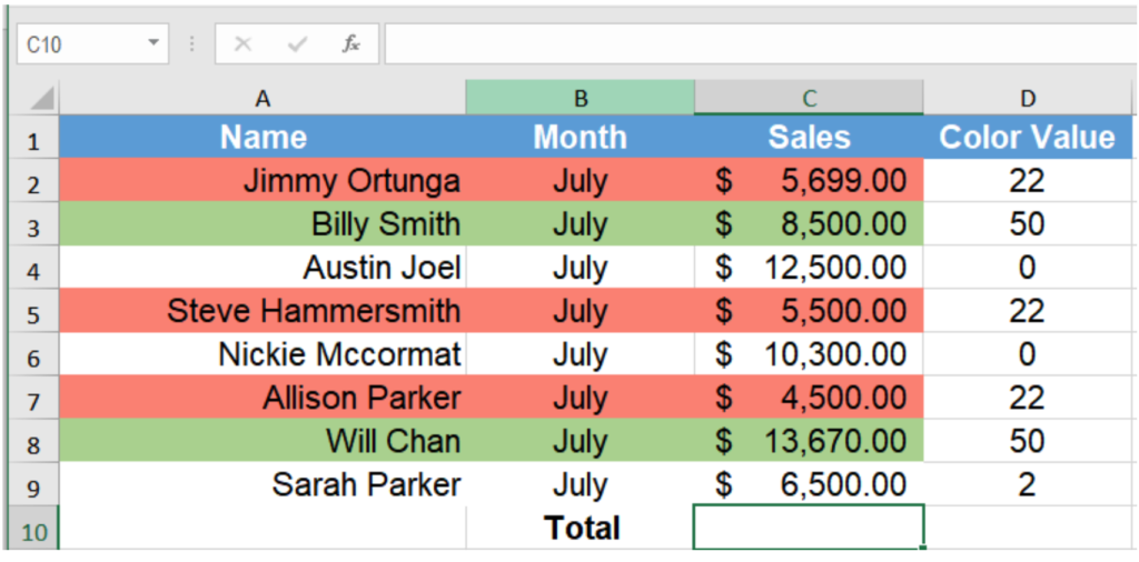
- Select cell D10 and assign the formula
= COUNTIF($D:$D, 22).
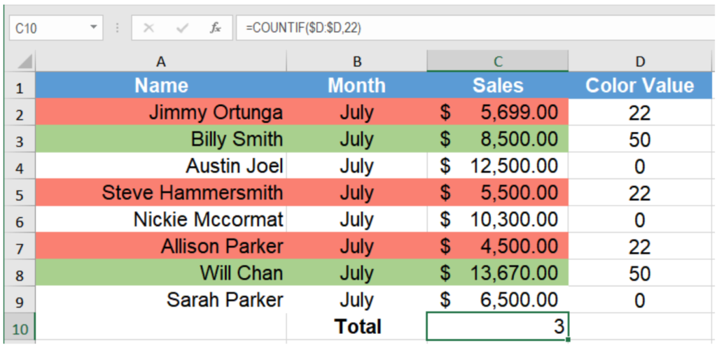
This will count the cells colored in red to find the number of salespersons with sales less than $7000 and return the number 3.
Using VBA
You can also create a custom function with VBA to count highlighted cells in Excel. To do that you need to create a custom function using VBA that works like a COUNTIF function and returns the number of cells for the same color.
You will follow the syntax: =CountFunction(CountColor, CountRange) and use it like other regular functions.Here CountColor is the color for which you want to count the cells. CountRange is the range in which you want to count the cells with the specified background color.
To count the cells highlighted in red, follow the steps below:
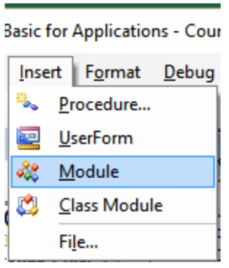
- Hold down the ALT + F11 keys, and it opens the Microsoft Visual Basic for Applications window.
- Click Insert > Module.
- Paste the following code in the Module Window.
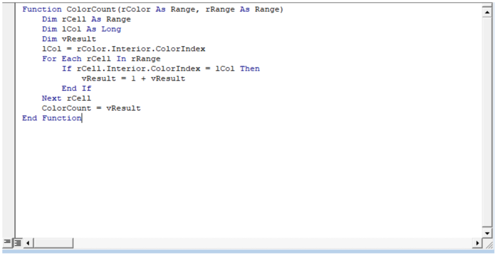
- In this code, you are defining a function with two arguments rColor and rRange. You are going to save the value of the background color of A2 in lCol. Then you are going to run a FOR loop where, if the cell’s background color matches the color in lCol, you increment vResult. This function returns the value of vResult, which is the count of the cells having the same background color.
- Then save the code, and apply the following formula to cell C10:
=ColorCount(A2, C2:C10).
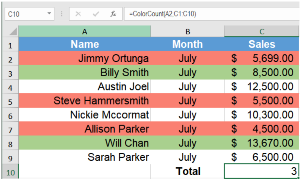
- Here A2 is the cell with the background color red you want to count. C2:C10 is the cell range that you want to count.
This will return the number of salespersons with sales less than $7000 in the month of July which is 3.
Содержание
- Count Colored Cells in Excel
- Top 3 Methods to Count Colored Cells In Excel
- #1 – Excel Count Colored Cells By Using Auto Filter Option
- #2 – Excel Count Colored Cells by using VBA Code
- #3 – Excel Count Colored Cells by Using FIND Method
- Things to Remember
- Recommended Articles
- How to Count Colored or Highlighted Cells in Excel
- Using Subtotal and Filter functions
- Using COUNTIF and GET.CELL functions
- Using VBA
- How to sum and count cells by color in Excel
- How to count cells by color in Excel
- Count cells by fill color
- Count cells by font color
- How to sum by color in Excel
- Sum values by cell color
- Sum values by font color
- Count and sum by color across entire workbook
- How to count colored cells in entire workbook
- How to sum colored cells in whole workbook
- Count and sum conditionally formatted cells
- How to count and sum conditionally formatted cells using VBA macro
- How to get cell color in Excel
- Get fill color of a cell
- Get font color of a cell
- Get hexadecimal color code of a cell
- How to insert VBA code in your workbook
- How to get custom functions to update
- Fastest way to calculate colored cells in Excel
- Sum and count cells by one color
- Count and sum all colored cells at once
Count Colored Cells in Excel


Top 3 Methods to Count Colored Cells In Excel
There is no built-in function to count colored cells in Excel, but below mentioned are three different methods to do this task.
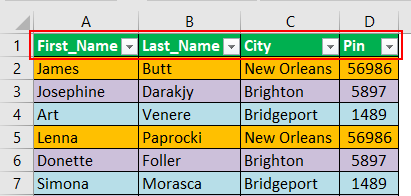
- Count colored cells by using the Auto Filter option
- Count colored cells by using the VBA code
- Count colored cells by using the FIND method
Table of contents
Now, let us discuss each of them in detail –
#1 – Excel Count Colored Cells By Using Auto Filter Option
For this example, let us look at the below data.
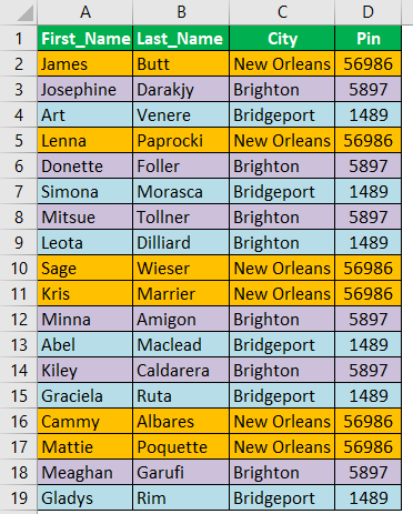
As we can see, each city is marked with different colors. So, we need to count the number of cities based on cell color.
As we can see, all the colors in the data. Now, we must choose the color that we want to filter.
We must follow the below steps to count cells by color.
At the bottom of the data, we need to apply the SUBTOTAL function in Excel to count cells.
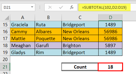
The SUBTOTAL function contains many formulas. It is helpful if we want to count, sum, and average only visible cell data. Under the heading PIN, we must click on the drop-down list filter and select Choose by Color.
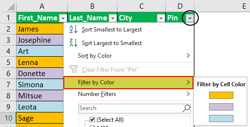
As we can see, all the colors in the data. Now, we must choose the color that we want to filter.

Wow. As we can see in cell D21, our SUBTOTAL function is given the count of filtered cells as 6 instead of the previous result of 18.
Similarly, now we must choose other colors to get the count of the same.

So, blue-colored cells count to five now.
#2 – Excel Count Colored Cells by using VBA Code
VBA’s street smart techniques help us reduce time consumption at our workplace for some complicated issues.
We can reduce time, but we can also create our functions to fit our needs. For example, we can create a function to count cells based on color in one such function. Below is the VBA code VBA Code VBA code refers to a set of instructions written by the user in the Visual Basic Applications programming language on a Visual Basic Editor (VBE) to perform a specific task. read more to create a function to count cells based on color.
Code:
Then, copy and paste the above code to your module.
The first line of the code “Color_Cell_Count” is the function name. Now, we must create three cells and color them as below.

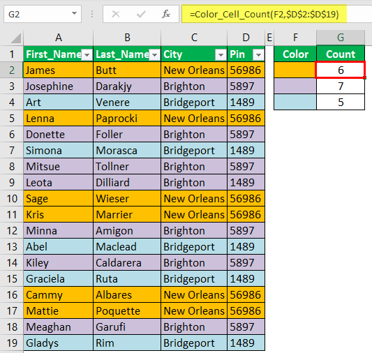
Now, we must open the function “Color_Cell_Count” in the G2 cell.
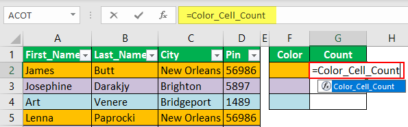
Even though we do not see the syntax of this function, the first argument is what color we need to count, so we must select cell F2.

The second argument is to select the range of cells as D2:D19.

Now, close the bracket and press the “Enter” key. As a result, it will provide the count of cells with the selected cell color.
Like this, with the help of UDF in VBA, we can count cells based on cell color.
#3 – Excel Count Colored Cells by Using FIND Method
We can also count cells based on the FIND method as well.
- Step 1: First, we must select the range of cells where we need to count cells.

- Step 2: Now, we need to press Ctrl + F to open the FIND dialog box.

- Step 3: Now, click on “Options>>.”

- Step 4: Consequently, it will expand the “Find” dialog box. Now, we must click on the “Format” option.

- Step 5: Now, it will open up the “Find Format” dialog box. We need to click on the “Choose Format From Cell” option.

- Step 6: Now, move the mouse pointer to see the pointer to select the format cell in excelFormat Cell In ExcelFormatting cells is an important technique to master because it makes any data presentable, crisp, and in the user’s preferred format. The formatting of the cell depends upon the nature of the data present.read more that we are looking to count.

- Step 7: We will select the cell formatted as the desired cell count. We have chosen the F2 cell as the desired cell format, and now we can see the preview.

- Step 8: Now, click on the “Find All” option to get the count of the selected cell format count of cells.

So, a total of 6 cells were found with selected formatting colors.
Things to Remember
- The provided VBA code is not a Subprocedure in VBASubprocedure In VBASUB in VBA is a procedure which contains all the code which automatically gives the statement of end sub and the middle portion is used for coding. Sub statement can be both public and private and the name of the subprocedure is mandatory in VBA.read more ; it is a UDF.
- The SUBTOTAL contains many formulas used to get the result only for visible cells when the filter is applied.
- We do not have any built-in function in Excel to count cells based on the color of the cell.
Recommended Articles
This article has been a guide to Count Colored Cells in Excel. We learned to count colored cells using the auto filter option, VBA code, FIND method, and downloadable Excel template. You may learn more about Excel from the following articles: –
Источник
How to Count Colored or Highlighted Cells in Excel
The COUNT function in Excel counts cells containing numbers in Excel. You cannot count colored or highlighted cells with the COUNT function. But you can follow a few workarounds to count colored cells in Excel. In this tutorial, you will learn how to count colored cells in Excel.
In excel, you can count highlighted cells using the following workarounds:
- Applying SUBTOTAL and filtering the data
- Using the COUNT and GET.CELL function
- Using VBA
Using Subtotal and Filter functions
You can count highlighted cells in Excel by subtotaling the visible cells and applying a filter based on colors.
In this example, you have the sales record for eight salespersons for the month of July. The rows containing salespersons having sales less than $7000 is highlighted in red, the other cells with the salespersons having a bonus is highlighted in green. To calculate the number of salespersons highlighted in red:
- Select the cell C10.
- Assign the formula = SUBTOTAL(102, C2:C9) . The first argument 102 counts the visible cells in the specified range.
- Select cells A1:C9 by clicking on cell A1 and dragging it till C9 with your mouse.
- Go to Data > Sort & Filter > Filter.
- Click on the filter drop downs in C1.
- Go to Filter by Color and select the color Red to find out the salespersons highlighted in red.
This will output change the subtotal value to x, which is the number of salespersons having sales less than $7000.
Using COUNTIF and GET.CELL functions
You can use GET.CELL with named ranges to count colored cells in Excel. GET.CELL is an old Macro4 function and does not work with regular functions. However, it still works with named ranges. To count colored cells with GET.CELL, you need to extract the color codes with GET.CELL and count them to find out the number of cells highlighted in the same color. To count cells using GET.CELL and COUNTIF:
- In the dialogue box that pops up, set name as ColorCount, scope as workbook and Refers to as =GET.CELL(38, Sheet1!C2).
- Assign the formula =ColorCount to cell D2 and drag it till D9 with your mouse.
- This would return a number based on the background color. If there is no background color, Excel would return 0. Otherwise all cells with the same background color return the same number.
- From column D, look at the code for the color red. In this case it is 22.
- Select cell D10 and assign the formula = COUNTIF($D:$D, 22).
This will count the cells colored in red to find the number of salespersons with sales less than $7000 and return the number 3.
Using VBA
You can also create a custom function with VBA to count highlighted cells in Excel. To do that you need to create a custom function using VBA that works like a COUNTIF function and returns the number of cells for the same color.
You will follow the syntax: =CountFunction(CountColor, CountRange) and use it like other regular functions.Here CountColor is the color for which you want to count the cells. CountRange is the range in which you want to count the cells with the specified background color.
To count the cells highlighted in red, follow the steps below:
- Hold down the ALT + F11 keys, and it opens the Microsoft Visual Basic for Applications window.
- Click Insert >Module .
- Paste the following code in the Module Window.
- In this code, you are defining a function with two arguments rColor and rRange . You are going to save the value of the background color of A2 in lCol. Then you are going to run a FOR loop where, if the cell’s background color matches the color in lCol, you increment vResult . This function returns the value of vResult, which is the count of the cells having the same background color.
- Then save the code, and apply the following formula to cell C10:
- Here A2 is the cell with the background color red you want to count. C2:C10 is the cell range that you want to count.
This will return the number of salespersons with sales less than $7000 in the month of July which is 3.
Источник
How to sum and count cells by color in Excel
 by Svetlana Cheusheva, updated on January 20, 2023
In this article, you will learn new effective approaches to summing and counting cells in Excel by color. These solutions work for cells colored manually and with conditional formatting in all versions of Excel 2010 through Excel 365.
Even though Microsoft Excel has a variety of functions for different purposes, none can calculate cells based on their color. Aside from third-party tools, there is only one efficient solution — create your own functions. If you know very little about user-defined functions or have never heard of this term before, don’t panic. The functions are already written and tested by us. All you need to do is to insert them in your workbook 🙂
How to count cells by color in Excel
Below, you can see the codes of two custom functions (technically, these are called user-defined functions or UDF). The first one is purposed for counting cells with a specific fill color and the other — font color. Both are written by Alex, one of our best Excel gurus.
Custom functions to count by color in Excel
Once the functions are added to your workbook, they will do all work behind the scenes, and you can use them in the usual way, just like any other native Excel function. From the end-user perspective, the functions have the following look.
Count cells by fill color
To count cells with a particular background color, this is the function to use:
- Data_range is a range in which to count cells.
- Cell_color is a reference to the cell with the target fill color.
To count cells of a specific color in a given range, carry out these steps:
- Insert the code of the CountCellsByColor function in your workbook.
- In a cell where you want the result to appear, start typing the formula: =CountCellsByColor(
- For the first argument, enter the range in which you want to count colored cells.
- For the second argument, supply the cell with the target color.
- Press the Enter key. Done!
For example, to find out how many cells in range B3:F24 have the same color as H3, the formula is:
In our sample dataset, the cells with values less than 150 are colored in yellow, and the cells with values higher than 350 in green. The function gets both counts with ease: 
Count cells by font color
In case your cell values have different font colors, you can count them using this function:
- Data_range is a range in which to count cells.
- Font_color is a reference to the cell with the sample font color.
For example, to get the number of cells in B3:F24 whose values have the same font color as H3, the formula is:
=CountCellsByFontColor(B3:F24, H3) 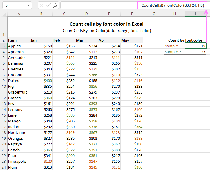
Tip. If you’d like to name the functions differently, feel free to change the names directly in the code.
How to sum by color in Excel
To sum colored values, add the following two functions to your workbook. As with the previous example, the first one handles fill color and the other — font color.
Custom functions to sum by color in Excel
Sum values by cell color
To sum by fill color in Excel, this is function to use:
- Data_range is a range in which to sum values.
- Cell_color is a reference to the cell with the fill color of interest.
For example, to add up the values of all cells in B3:F24 that are shaded with the same color as H3, the formula is:
=SumCellsByColor(B3:F24, H3) 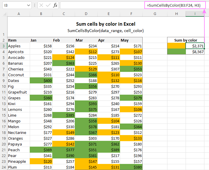
Sum values by font color
To sum numeric values with a specific font color, use this function:
- Data_range is a range in which to sum cells.
- Font_color is a reference to the cell with the target font color.
For instance, to add up all the values in cells B3:F24 with the same font color as the value in H3, the formula is:
=SumCellsByFontColor(B3:F24, H3) 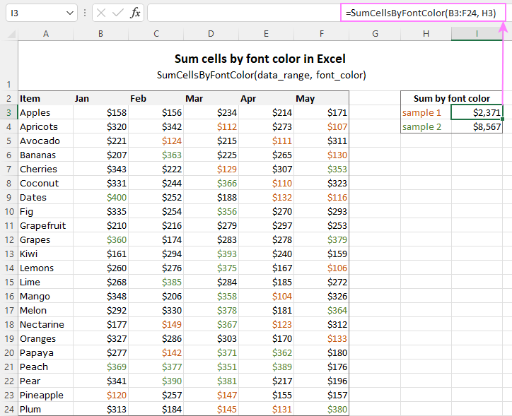
Count and sum by color across entire workbook
To count and sum cells of a certain color in all sheets of a given workbook, we created two separate functions, which are named WbkCountByColor and WbkSumByColor, respectively. Here comes the code:
Custom functions to count and sum by color across workbook
Note. To make the functions’ code more compact, we refer to the two previously discussed functions that count and sum within a specified range. So, for the «workbook functions» to work, be sure to add the code of the CountCellsByColor and SumCellsByColor functions to your Excel too.
How to count colored cells in entire workbook
To find out how many cells of a particular color there are in all sheets of a given workbook, use this function:
The function takes just one argument — a reference to any cell filled with the color of interest. So, a real-life formula may look something like this:
Where A1 is the cell with the sample fill color.
How to sum colored cells in whole workbook
To get a total of values in all cells of the current workbook highlighted with a particular color, use this function:
Assuming the target color is in cell B1, the formula takes this form:
Count and sum conditionally formatted cells
The custom functions for adding up and counting color-coded cells are really nice, aren’t they? The problem is that they do not work for cells colored with conditional formatting, alas 🙁
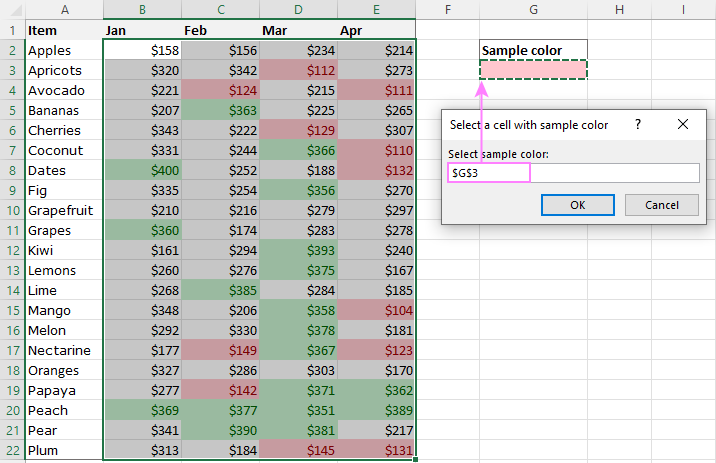
To handle conditional formatting, we have written a different code (kudos to Alex again!). It works well with both preset formats and custom formula-based rules. Contrasting with the previous examples, this code is a macro, not a function. The macro counts and sums conditionally formatted cells by fill color. Please insert it in your VBA Editor, and then follow the below instructions.
VBA macro to count and sum conditionally formatted cells.
How to count and sum conditionally formatted cells using VBA macro
With the macro’s code inserted in your Excel, this is what you need to do:
- Select one or more ranges where you want to count and sum colored cells. Make sure the selected range(s) contains numerical data.
- Press Alt + F8 , select the SumCountByConditionalFormat macro in the list, and click Run.
- A small dialog box will pop asking you to select a cell with the sample color. Do this and click OK.
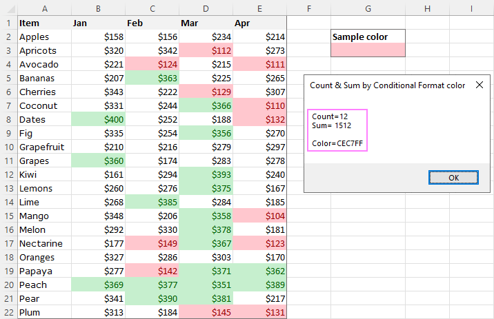
For this example, we used the inbuilt Highlight Cell Rules and got the following results:
- Count (12) the number of cells in range B2:E22 with the same color as G3.
- Sum (1512) is the sum of values in cells formatted with Light Red Fill.
- Color is a hexadecimal color code of the sample cell.
Tip. The sample workbook with the SumCountByConditionalFormat macro is available for download at the end of this post.
How to get cell color in Excel
If you need (or are curious) to know the color of a specific cell (fill or font color), add the following user-defined functions to your Excel. It returns ColorIndex as a decimal number.
Custom functions to get the cell color
Note. The functions only work for colors applied manually, and not with conditional formatting.
Get fill color of a cell
To return a decimal code of the color a given cell is highlighted with, make use of this function:
For example, to get the color of cell A2, the formula is:
Get font color of a cell
To get a font color of a cell, use an analogous function:
For instance, to find the font color of cell E2, the formula is:
Get hexadecimal color code of a cell
To convert a decimal color index returned by our custom functions into a hexadecimal color code, make use of Excel’s native DEC2HEX function.
=»#»&DEC2HEX(GetFontColor(E2)) 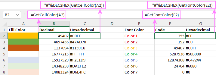
How to insert VBA code in your workbook
To add the function’s or macro’s code to your Excel, move on with these 4 steps:
- In your workbook, press Alt + F11 to open Visual Basic Editor.
- In the left pane, right-click on the workbook name, and then choose Insert >Module from the context menu.
- In the Code window, insert the code of the desired function(s):
- Count by color: CountCellsByColor and CountCellsByFontColor functions
- Sum by color: SumCellsByColor and SumCellsByFontColor functions
- Count and sum colored cells in whole workbook: WbkCountByColor and WbkSumByColor functions
- Count and sum conditionally formatted cells: SumCountByConditionalFormat function
- Get color code: GetCellColor and GetFontColor functions
- Save your file as Macro-Enabled Workbook (.xlsm).
If you are not very comfortable with VBA, you can find the detailed step-by-step instructions and a handful of useful tips in this tutorial: How to insert and run VBA code in Excel.
How to get custom functions to update
When summing and counting color-coded cells in Excel, please keep in mind that your formulas won’t recalculate automatically after coloring a few more cells or changing existing colors. Please don’t be angry with us, this is not a bug in our code 🙂
The point is that changing cell color in Excel does not trigger worksheet recalculation. To get the formulas to update, press either F9 to recalculate all open workbooks or Shift + F9 to recalculate only the active sheet. Or just place the cursor into any cell and press F2, and then hit Enter. For more information, please see How to force recalculation in Excel.
Fastest way to calculate colored cells in Excel
If you do not want to waste time tinkering with VBA codes, I’m happy to introduce you to our very simple but powerful Count & Sum by Color tool. Together with 70+ other time-saving add-ins, it is included with Ultimate Suite for Excel.
Once installed, you will find it on the Ablebits Tools tab of your Excel ribbon: 
And here is a short summary of what the Count & Sum by Color add-in can do:
- Count and sum cells by color in all versions of Excel 2016 — Excel 365.
- Find average, maximum and minimum values in the colored cells.
- Handle cells colored manually and with conditional formatting.
- Paste the results anywhere in a worksheet as values or formulas.
Sum and count cells by one color
Selecting the Sum & Count by One Color option will open the following pane in the left part of your worksheet. You specify the source range and sample cell, then then click Calculate.
The result will appear on the pane straight away! No macros, no formulas, no pain 🙂
Apart from count and sum, the add-in also shows Average, Max and Min for colored numbers. To insert a particular value in the sheet, click the Paste button next to it. Or click Paste All to have all the results inserted at once: 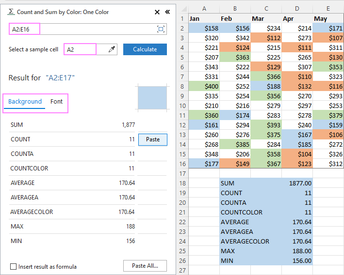
Count and sum all colored cells at once
To handle all colored cells at a time, choose the Sum & Count by All Color option. Basically, it works in the same way, except that instead of color, you choose the function to calculate. 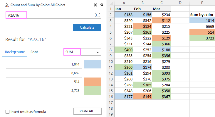
Tip. To have the results inserted in the worksheet as formulas (custom functions), check the corresponding box at the bottom of the pane.
Well, calculating colored cells in Excel is pretty easy, isn’t it? Of course, if you have that little gem that makes the magic happen 🙂 Curious to see how our add-in will cope with your colored cells? The download link is right below.
Источник