
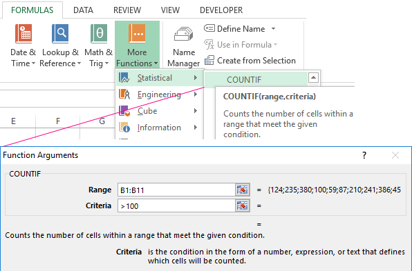
COUNTIF function
Use COUNTIF, one of the statistical functions, to count the number of cells that meet a criterion; for example, to count the number of times a particular city appears in a customer list.
In its simplest form, COUNTIF says:
-
=COUNTIF(Where do you want to look?, What do you want to look for?)
For example:
-
=COUNTIF(A2:A5,»London»)
-
=COUNTIF(A2:A5,A4)

COUNTIF(range, criteria)
|
Argument name |
Description |
|---|---|
|
range (required) |
The group of cells you want to count. Range can contain numbers, arrays, a named range, or references that contain numbers. Blank and text values are ignored. Learn how to select ranges in a worksheet. |
|
criteria (required) |
A number, expression, cell reference, or text string that determines which cells will be counted. For example, you can use a number like 32, a comparison like «>32», a cell like B4, or a word like «apples». COUNTIF uses only a single criteria. Use COUNTIFS if you want to use multiple criteria. |
Examples
To use these examples in Excel, copy the data in the table below, and paste it in cell A1 of a new worksheet.
|
Data |
Data |
|---|---|
|
apples |
32 |
|
oranges |
54 |
|
peaches |
75 |
|
apples |
86 |
|
Formula |
Description |
|
=COUNTIF(A2:A5,»apples») |
Counts the number of cells with apples in cells A2 through A5. The result is 2. |
|
=COUNTIF(A2:A5,A4) |
Counts the number of cells with peaches (the value in A4) in cells A2 through A5. The result is 1. |
|
=COUNTIF(A2:A5,A2)+COUNTIF(A2:A5,A3) |
Counts the number of apples (the value in A2), and oranges (the value in A3) in cells A2 through A5. The result is 3. This formula uses COUNTIF twice to specify multiple criteria, one criteria per expression. You could also use the COUNTIFS function. |
|
=COUNTIF(B2:B5,»>55″) |
Counts the number of cells with a value greater than 55 in cells B2 through B5. The result is 2. |
|
=COUNTIF(B2:B5,»<>»&B4) |
Counts the number of cells with a value not equal to 75 in cells B2 through B5. The ampersand (&) merges the comparison operator for not equal to (<>) and the value in B4 to read =COUNTIF(B2:B5,»<>75″). The result is 3. |
|
=COUNTIF(B2:B5,»>=32″)-COUNTIF(B2:B5,»<=85″) |
Counts the number of cells with a value greater than (>) or equal to (=) 32 and less than (<) or equal to (=) 85 in cells B2 through B5. The result is 1. |
|
=COUNTIF(A2:A5,»*») |
Counts the number of cells containing any text in cells A2 through A5. The asterisk (*) is used as the wildcard character to match any character. The result is 4. |
|
=COUNTIF(A2:A5,»?????es») |
Counts the number of cells that have exactly 7 characters, and end with the letters «es» in cells A2 through A5. The question mark (?) is used as the wildcard character to match individual characters. The result is 2. |
Common Problems
|
Problem |
What went wrong |
|---|---|
|
Wrong value returned for long strings. |
The COUNTIF function returns incorrect results when you use it to match strings longer than 255 characters. To match strings longer than 255 characters, use the CONCATENATE function or the concatenate operator &. For example, =COUNTIF(A2:A5,»long string»&»another long string»). |
|
No value returned when you expect a value. |
Be sure to enclose the criteria argument in quotes. |
|
A COUNTIF formula receives a #VALUE! error when referring to another worksheet. |
This error occurs when the formula that contains the function refers to cells or a range in a closed workbook and the cells are calculated. For this feature to work, the other workbook must be open. |
Best practices
|
Do this |
Why |
|---|---|
|
Be aware that COUNTIF ignores upper and lower case in text strings. |
|
|
Use wildcard characters. |
Wildcard characters —the question mark (?) and asterisk (*)—can be used in criteria. A question mark matches any single character. An asterisk matches any sequence of characters. If you want to find an actual question mark or asterisk, type a tilde (~) in front of the character. For example, =COUNTIF(A2:A5,»apple?») will count all instances of «apple» with a last letter that could vary. |
|
Make sure your data doesn’t contain erroneous characters. |
When counting text values, make sure the data doesn’t contain leading spaces, trailing spaces, inconsistent use of straight and curly quotation marks, or nonprinting characters. In these cases, COUNTIF might return an unexpected value. Try using the CLEAN function or the TRIM function. |
|
For convenience, use named ranges |
COUNTIF supports named ranges in a formula (such as =COUNTIF(fruit,»>=32″)-COUNTIF(fruit,»>85″). The named range can be in the current worksheet, another worksheet in the same workbook, or from a different workbook. To reference from another workbook, that second workbook also must be open. |
Note: The COUNTIF function will not count cells based on cell background or font color. However, Excel supports User-Defined Functions (UDFs) using the Microsoft Visual Basic for Applications (VBA) operations on cells based on background or font color. Here is an example of how you can Count the number of cells with specific cell color by using VBA.
Need more help?
You can always ask an expert in the Excel Tech Community or get support in the Answers community.

See also
COUNTIFS function
IF function
COUNTA function
Overview of formulas in Excel
IFS function
SUMIF function
Need more help?
Want more options?
Explore subscription benefits, browse training courses, learn how to secure your device, and more.
Communities help you ask and answer questions, give feedback, and hear from experts with rich knowledge.
The COUNTIF function counts cells in a range that meet a given condition, referred to as criteria. COUNTIF is a common, widely used function in Excel, and can be used to count cells that contain dates, numbers, and text. Note that COUNTIF can only apply a single condition. To count cells with multiple criteria, see the COUNTIFS function.
Syntax
The generic syntax for COUNTIF looks like this:
=COUNTIF(range,criteria)The COUNTIF function takes two arguments, range and criteria. Range is the range of cells to apply a condition to. Criteria is the condition to apply, along with any logical operators that are needed.
Applying criteria
The COUNTIF function supports logical operators (>,<,<>,<=,>=) and wildcards (*,?) for partial matching. The tricky part about using the COUNTIF function is the syntax used to apply criteria. COUNTIFS is in a group of eight functions that split logical criteria into two parts, range and criteria. Because of this design, each condition requires a separate range and criteria argument, and operators in the criteria must be enclosed in double quotes («»). The table below shows examples of the syntax needed for common criteria:
| Target | Criteria |
|---|---|
| Cells greater than 75 | «>75» |
| Cells equal to 100 | 100 or «100» |
| Cells less than or equal to 100 | «<=100» |
| Cells equal to «Red» | «red» |
| Cells not equal to «Red» | «<>red» |
| Cells that are blank «» | «» |
| Cells that are not blank | «<>» |
| Cells that begin with «X» | «x*» |
| Cells less than A1 | «<«&A1 |
| Cells less than today | «<«&TODAY() |
Notice the last two examples involve concatenation with the ampersand (&) character. Any time you are using a value from another cell, or using the result of a formula in criteria with a logical operator like «<«, you will need to concatenate. This is because Excel needs to evaluate cell references and formulas first to get a value, before that value can be joined to an operator.
Basic example
In the worksheet shown above, the following formulas are used in cells G5, G6, and G7:
=COUNTIF(D5:D12,">100") // count sales over 100
=COUNTIF(B5:B12,"jim") // count name = "jim"
=COUNTIF(C5:C12,"ca") // count state = "ca"
Notice COUNTIF is not case-sensitive, «CA» and «ca» are treated the same.
Double quotes («») in criteria
In general, text values need to be enclosed in double quotes («»), and numbers do not. However, when a logical operator is included with a number, the number and operator must be enclosed in quotes, as seen in the second example below:
=COUNTIF(A1:A10,100) // count cells equal to 100
=COUNTIF(A1:A10,">32") // count cells greater than 32
=COUNTIF(A1:A10,"jim") // count cells equal to "jim"
Value from another cell
A value from another cell can be included in criteria using concatenation. In the example below, COUNTIF will return the count of values in A1:A10 that are less than the value in cell B1. Notice the less than operator (which is text) is enclosed in quotes.
=COUNTIF(A1:A10,"<"&B1) // count cells less than B1
Not equal to
To construct «not equal to» criteria, use the «<>» operator surrounded by double quotes («»). For example, the formula below will count cells not equal to «red» in the range A1:A10:
=COUNTIF(A1:A10,"<>red") // not "red"
Blank cells
COUNTIF can count cells that are blank or not blank. The formulas below count blank and not blank cells in the range A1:A10:
=COUNTIF(A1:A10,"<>") // not blank
=COUNTIF(A1:A10,"") // blank
Note: be aware that COUNTIF treats formulas that return an empty string («») as not blank. See this example for some workarounds to this problem.
Dates
The easiest way to use COUNTIF with dates is to refer to a valid date in another cell with a cell reference. For example, to count cells in A1:A10 that contain a date greater than the date in B1, you can use a formula like this:
=COUNTIF(A1:A10, ">"&B1) // count dates greater than A1
Notice we must concatenate an operator to the date in B1. To use more advanced date criteria (i.e. all dates in a given month, or all dates between two dates) you’ll want to switch to the COUNTIFS function, which can handle multiple criteria.
The safest way to hardcode a date into COUNTIF is to use the DATE function. This ensures Excel will understand the date. To count cells in A1:A10 that contain a date less than April 1, 2020, you can use a formula like this
=COUNTIF(A1:A10,"<"&DATE(2020,4,1)) // dates less than 1-Apr-2020
Wildcards
The wildcard characters question mark (?), asterisk(*), or tilde (~) can be used in criteria. A question mark (?) matches any one character and an asterisk (*) matches zero or more characters of any kind. For example, to count cells in A1:A5 that contain the text «apple» anywhere, you can use a formula like this:
=COUNTIF(A1:A5,"*apple*") // cells that contain "apple"
To count cells in A1:A5 that contain any 3 text characters, you can use:
=COUNTIF(A1:A5,"???") // cells that contain any 3 characters
The tilde (~) is an escape character to match literal wildcards. For example, to count a literal question mark (?), asterisk(*), or tilde (~), add a tilde in front of the wildcard (i.e. ~?, ~*, ~~).
OR logic
The COUNTIF function is designed to apply just one condition. However, to count cells that contain «this OR that», you can use an array constant and the SUM function like this:
=SUM(COUNTIF(range,{"red","blue"})) // red or blue
The formula above will count cells in range that contain «red» or «blue». Essentially, COUNTIF returns two counts in an array (one for «red» and one for «blue») and the SUM function returns the sum. For more information, see this example.
Limitations
The COUNTIF function has some limitations you should be aware of:
- COUNTIF only supports a single condition. If you need to count cells using multiple criteria, use the COUNTIFS function.
- COUNTIF requires an actual range for the range argument; you can’t provide an array. This means you can’t alter values in range before applying criteria.
- COUNTIF is not case-sensitive. Use the EXACT function for case-sensitive counts.
- COUNTIFS has other quirks explained in this article.
The most common way to work around the limitations above is to use the SUMPRODUCT function. In the current version of Excel, another option is to use the newer BYROW and BYCOL functions.
Notes
- Text strings in criteria must be enclosed in double quotes («»), i.e. «apple», «>32», «app*»
- Cell references in criteria are not enclosed in quotes, i.e. «<«&A1
- The wildcard characters ? and * can be used in criteria. A question mark matches any one character and an asterisk matches any sequence of characters (zero or more).
- To match a literal question mark(?) or asterisk (*), use a tilde (~) like (~?, ~*).
- COUNTIF requires a range, you can’t substitute an array.
- COUNTIF returns incorrect results when used to match strings longer than 255 characters.
- COUNTIF will return a #VALUE error when referencing another workbook that is closed.
The COUNTIF function is included in the group of statistical functions. It allows you to find the number of cells by a certain criterion. The COUNTIF function works with numeric and text values, as well as with dates.
Syntax and features of the function
First, let’s consider the arguments:
- Range – the group of values for analysis and counting (required).
- Criteria – the condition by which cells are to be counted (required).
The range of cells can include textual and numerical values, dates, arrays, and references to numbers. The function ignores empty cells.
A criterion can be a reference, a number, a text string, or an expression. The COUNTIF function only works with one criterion (by default). However, you can “force” it to analyze two criteria simultaneously.
Recommendations for the correct operation of the function:
- If the COUNTIF function refers to a range in another workbook, this workbook must be opened.
- The «Criteria» argument must be enclosed in quotation marks (except for references).
- The function does not take into account the letter case.
- When formulating a counting condition, you can use wildcard characters. The question mark «?» is any character. The asterisk «*» is any sequence of characters. For the formula to search for these signs directly, put a tilde (~) before them.
- For normal operation of the formula, cells with text values should not contain spaces or non-printable characters.
Countif function in Excel: examples
Let’s count the numerical values in one range. The counting condition is one criterion.
We have the following table:
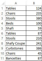
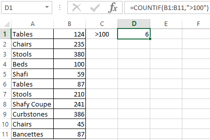
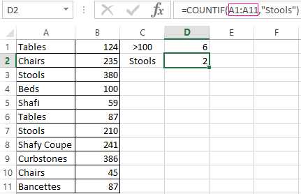
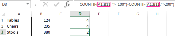
Count the number of cells with numbers greater than 100. Formula: =COUNTIF(B1:B11,»>100″). The range is В1:В11. The counting criterion is «>100». The result:
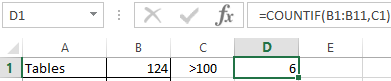
If the counting condition is entered in a separate cell, you can use the reference as a criterion:
Count the text values in one range. The search condition is one criterion. Formula: =COUNTIF(A1:A11,A3).
Or used reference inside the table:
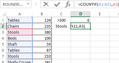
In the second case, the cell reference was used as a criterion, result is the same – 2.
Formula with the wildcard character application: =COUNTIF(A1:A11,»Tab*»). To calculate the number of values ending in «и» and containing any number of characters: =COUNTIF(A1:A11,»*s»). We obtain:
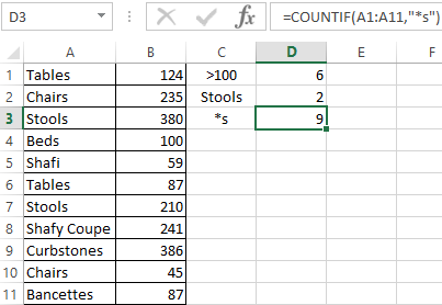
All names that end with a letter «s».
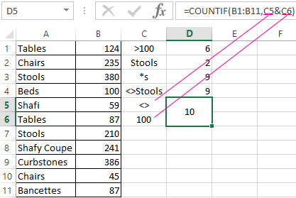
We use the search condition «not equal» in the COUNTIF.
Formula: =COUNTIF(A1:A11,»<>»&»Stools»). The operator «<>» means «not equal». The ampersand sign (&) is used to merge this operator and the “Stools” value.
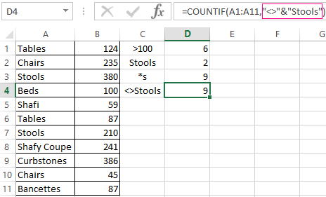
When you apply a reference, the formula will look like this:
Often you need to perform the COUNTIF function in Excel by two criteria. In this way, you can significantly expand its capabilities. Let’s consider special cases of using the COUNTIF function in Excel and examples with two criteria.
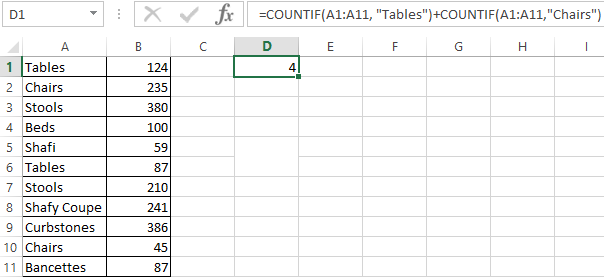
- Let’s count how many cells are contained in the » Tables » and » Chairs » text. Formula:
To specify several criteria, several COUNTIF phrases are used. They are united by the «+» operator.
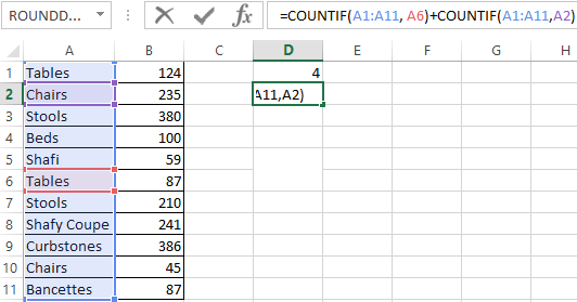
- Criteria – cell references. Formula:
The function searches for » Tables » text in cell A1 and » Chairs » text – in cell A2 based on the criterion.
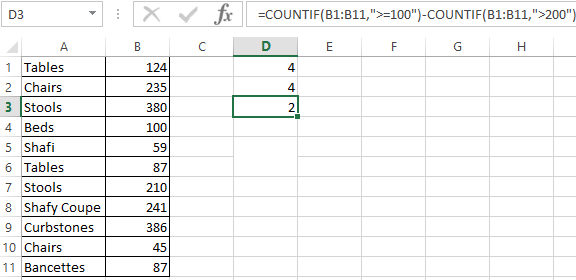
- Count the number of cells in B1:B11 range with a value greater than or equal to 100 and less than or equal to 200. Formula:
- Apply several ranges in the COUNTIF function. This is possible if the ranges are contiguous. It searches for values by two criteria in two columns simultaneously. If the ranges are not adjacent, then the COUNTIFS function is used.
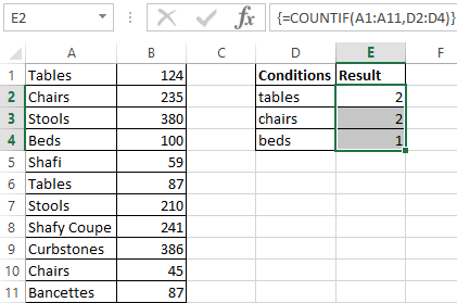
- When the criterion is a reference to a range of cells with conditions, the function returns the array. To enter a formula, you need to highlight as many cells as the range with criteria contains. After entering the arguments, simultaneously press Shift + Ctrl + Enter control key combination. Excel recognizes the formula of the array.
COUNTIF with two criteria in Excel is very often used for automated and efficient data handling. Therefore, an advanced user is highly recommended to carefully study all of the examples above.
Subtotal command and the countif function
Count the number of goods sold in groups.
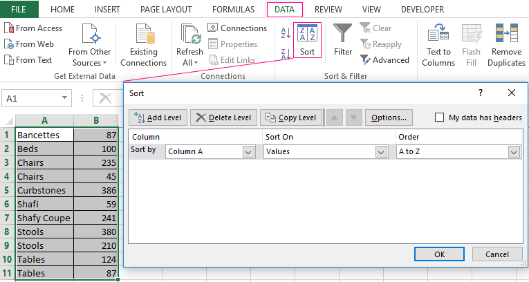
- First, sort the table so that the same values are close.
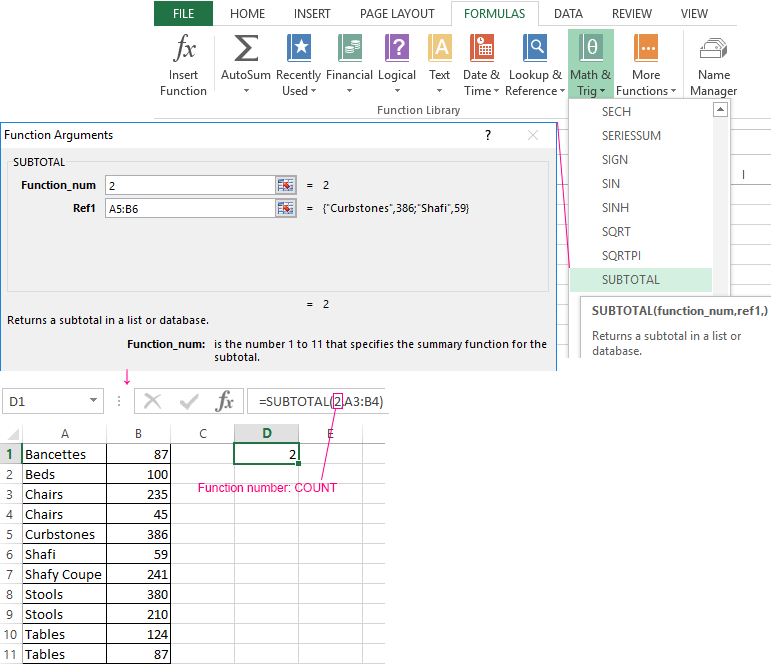
- The first argument of the formula “SUBTOTAL” – “Function number”. These are numbers from 1 to 11, indicating a statistical function for calculating the intermediate result. Counting the number of cells is carried out under number «2» (“COUNT”).
Download example COUNTIF in Excel
The formula has found the number of values for the «Chairs» group. For a large number of rows (more than a thousand), this combination of functions can be useful.
I would like to include an "AND" condition for one of the conditions I have in my COUNTIFS clause.
Something like this:
=COUNTIFS(A1:A196;{"Yes"or "NO"};J1:J196;"Agree")
So, it should return the number of rows where:
(A1:A196 is either "yes" or "no") AND (J1:j196 is "agree")
![]()
apomene
14.3k9 gold badges46 silver badges71 bronze badges
asked May 14, 2014 at 13:08
![]()
You could just add a few COUNTIF statements together:
=COUNTIF(A1:A196,"yes")+COUNTIF(A1:A196,"no")+COUNTIF(J1:J196,"agree")
This will give you the result you need.
EDIT
Sorry, misread the question. Nicholas is right that the above will double count. I wasn’t thinking of the AND condition the right way. Here’s an alternative that should give you the correct results, which you were pretty close to in the first place:
=SUM(COUNTIFS(A1:A196,{"yes","no"},J1:J196,"agree"))
answered May 14, 2014 at 13:28
![]()
tmoore82tmoore82
1,8471 gold badge27 silver badges48 bronze badges
11
There is probably a more efficient solution to your question, but following formula should do the trick:
=SUM(COUNTIFS(J1:J196,"agree",A1:A196,"yes"),COUNTIFS(J1:J196,"agree",A1:A196,"no"))
answered May 14, 2014 at 13:29
![]()
Nicholas FleesNicholas Flees
1,9333 gold badges23 silver badges30 bronze badges
4
In a more general case:
N( A union B) = N(A) + N(B) - N(A intersect B)
= COUNTIFS(A1:A196,"Yes",J1:J196,"Agree")+COUNTIFS(A1:A196,"No",J1:J196,"Agree")-A1:A196,"Yes",A1:A196,"No")
![]()
answered Jun 26, 2017 at 2:12
![]()
AdelAdel
1416 bronze badges
One solution is doing the sum:
=SUM(COUNTIFS(A1:A196,{"yes","no"},B1:B196,"agree"))
or know its not the countifs but the sumproduct will do it in one line:
=SUMPRODUCT(((A1:A196={"yes","no"})*(j1:j196="agree")))
answered May 14, 2014 at 14:22
![]()
GregGreg
1415 bronze badges
Using array formula.
=SUM(COUNT(IF(D1:D5="Yes",COUNT(D1:D5),"")),COUNT(IF(D1:D5="No",COUNT(D1:D5),"")),COUNT(IF(D1:D5="Agree",COUNT(D1:D5),"")))
PRESS = CTRL + SHIFT + ENTER.
answered May 14, 2014 at 13:59
![]()
1
i found i had to do something akin to
=(countifs (A1:A196,"yes", j1:j196, "agree") + (countifs (A1:A196,"no", j1:j196, "agree"))
![]()
answered Sep 21, 2015 at 10:08
![]()
1
Excel tables with their functions come in handy to count cells with data, horizontally and vertically. COUNTIF is the common function for counting cells with one and several conditions. So let’s look into this further to understand all the details and distinctions.
Meaning of COUNTIF Excel
COUNTIF in Excel is a statistical function that counts cells with those data that users indicate. It takes into account one condition.
- You can find items recorded even for months under a specific name.
- You may count the number of cells that hold a common letter or sign.
- You can use the Excel COUNTIF not blank to learn the empty cells quantity.
- You specify numerosity more or less than a mentioned value.
The COUNTIF formula in Excel consists of range (which goes first) and criteria (indicates the corresponding position).
=COUNTIF (range, criterion) rangeis the mandatory argument, which includes cells needed to find.criterionincludes expression, word, figures, letter, or other conditions that you need to discover.
How to use COUNTIF in Excel?
The function works with only one condition. Nevertheless, a person may single out many different data in turn. The computation is carried out with numbers, letters, words, phrases and dates. You can only write a cell reference or an entire condition. Sometimes, wildcards and symbols assist to determine more accurate values.
How COUNTIF works in Excel?
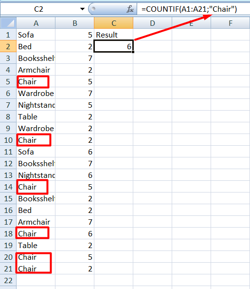
The function calculates the number of cells with indicated context, i.e., with the data that the user needs to count. For instance, you have a chart with diversified furniture bought over time. You may count what furniture (sofa, bed, wardrobe, chair, table, etc.) people buy. The COUNTIF will compute the cells in which the mentioned furniture is located. You write down the formula according to the condition you ought to detect. For example, let’s count the number of cells containing the word ‘chair‘:
=COUNTIF(A1:A21,"Chair")
Does COUNTIF function in Excel work for several criteria?
The COUNTIF doesn’t support frequentative conditions. Thus, you won’t find the number of chairs or nightstands purchased only in January or only on February 3. You have to use COUNTIFS for such cases.
However, you may write COUNTIF + COUNTIF. Such a COUNTIF Excel multiple criteria function makes the outcome more complete. Let’s determine the number of purchased chairs and sofas. Write the following:
=COUNTIF(A2:A21,"Chair")+COUNTIF(A2:A21,"Sofa").

Samples of advanced COUNTIFS function in Excel
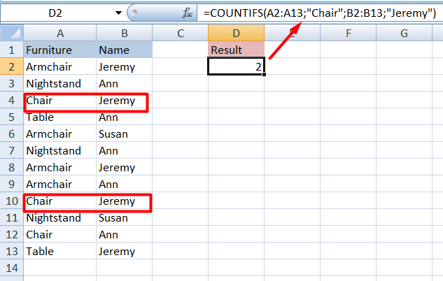
COUNTIF and COUNTIFS are various functions. They differ in the computation of cells with one criterion or more criteria. The first identifies cells under one condition, and the second takes into account several specific criteria. Let’s count the number of chairs bought by Jeremy. We need to use COUNTIFS for such appointments. Write it as follows:
=COUNTIFS(A2:A13,"Chair",B2:B13,"Jeremy")
Using COUNTIF in Excel when data is on other sources
People usually store data on certain apps, such as Harvest, Google Drive, Jira, Pipedrive, etc. When you need to calculate this data in Excel, you can import it from the app. The Coupler.io tool is designed exactly for this. It will help transfer all the necessary information to BigQuery, Google Sheets, or Excel from other sources. In addition, you can automate updates to make your work easier in the future.

Sign up to Coupler.io and complete two steps to set up your Excel integration: source and destination. If you want to schedule automatic data refresh, you’ll need to configure one more step – schedule. Here is what the integration may look like:

Practical skills based on a COUNTIF Excel example
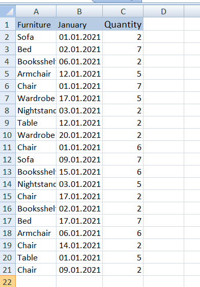
Examine a few samples of use in more detail. Take, for instance, the furniture in the store. Imagine the owner created an Excel table regarding sales. They write down the furniture in one column there. The other column contains the dates when the goods were sold. Finally, the third column contains the quantity of each product sold. So, let’s define some samples with several formulas, including dates, words and figures.
Excel COUNTIF: Cells are equal or not equal
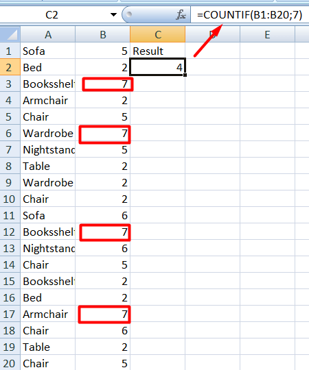
Imagine that people have bought every subject several times. Let’s take, for example, 7 times. In our formula, we specify the range where to look and the figure 7.
=COUNTIF(B1:B20,7)
Let’s still find the purchased furniture that isn’t equal to 5.
=COUNTIF(B1:B20,"<>5")

Excel COUNTIF: cells contain words
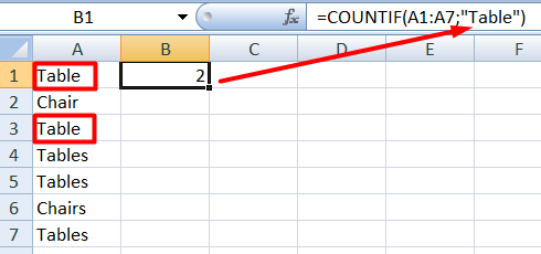
Let’s try to work with words using the same formula. Imagine that we need to know how many tables people bought. Let’s write the following formula.
=COUNTIF(A2:A21,"Table")

As a result, people bought 2 tables. You can replace the word with a cell reference
=COUNTIF(A2:A21,E2)

COUNTIF use in Excel – meaning of wildcards
We can use COUNTIF not only with words but also with special wildcards (* and ?) to generalize the condition.
?= One character.*= Sequence.
Also, you can write ~ to find symbols * or ?.
Let’s look at a simple formula
=COUNTIF(A1:A7,"Table")
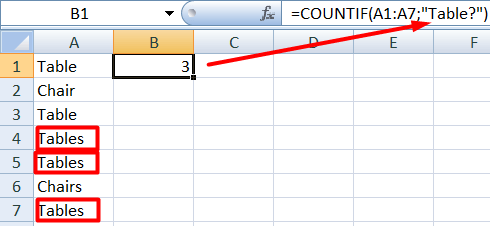
The question mark symbol ? adds one additional character. In our dataset, there are the words ‘Table‘ and ‘Tables‘ with the last letter ‘s‘. So, Table? in the formula will look for the latter option:
=COUNTIF(A1:A7,"Table?")
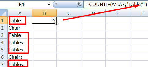
The asterisk symbol * adds a sequence of characters or even spaces. For instance, the following formula counts all words that start with Tab including ‘Table’ and ‘Tables’:
=COUNTIF(A1:A7,"Tab*")
Excel COUNTIF: сells are more than or less than
Let’s find out some values using operators: >, <, <>, =. We write it next to the criterion in quotation marks. Thanks to them, we can find cells with numbers that are more or less, equal, or not equal to some value. For example, let’s count the amount of furniture that people bought more than 3 times:
=COUNTIF(B1:B20,">3")

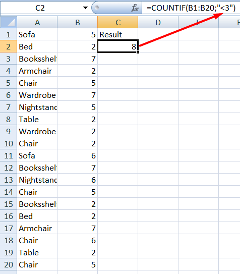
Change the logical operator to count the amount of furniture that people bought less than 3 times:
=COUNTIF(B1:B20,"<3")
Excel COUNTIF: count cells including date
Another feature is working with dates. So, let’s imagine that the biggest purchases fall on the date of January 1. We need to know the cells’ numerosity with this data.
=COUNTIF(B2:B21,"01/01/2021")

What common problems should you avoid?
Often, people face issues using the function. We seem to be doing everything right, but the Excel function COUNTIF shows the error. Look at a few situations why it occurs. For instance, you wrote the formula
=COUNTIF(A2:A13,Chair)
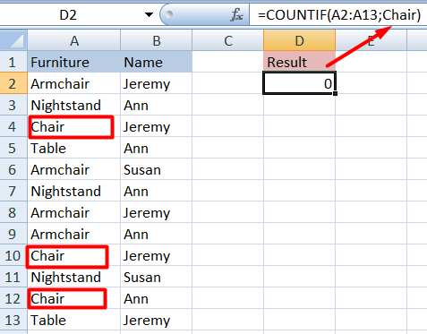
The function has shown zero results although this is not correct. So taking a closer look, the word ‘Chair‘ should be in quotation marks.
=COUNTIF(A2:A13,"Chair")
In another example of incorrect syntax, the formula returned #NAME?. In this case, there is a space between the range (A1:A7) and the criterion, which also has not quotation marks (Table).

The correct formula should look like this
=COUNTIF(A1:A7,"Table")
Best practices in using the COUNTIF function
It is easy to make mistakes both out of ignorance and inattention. However, by applying the following tips you can avoid the common mistakes.
- Write the wildcards (
?and*) to generalize the condition. - The condition can only have less than 255 characters. You will see an error exceeding this limit. To exceed the limit, you can use CONCATENATE or ampersand (&).
- The function returns the same value if the words are written in uppercase or lowercase letters. It doesn’t take into account case strings. You should rename the word if it has a different meaning.
- Pay attention to the spelling of words and letters. The function does not differentiate case strings and doesn’t work with misspellings.
Adherence to all principles and rules and writing correct syntax will facilitate calculations without problems. The main point is to write the formula and condition correctly.
-

Technical Content Writer on Coupler.io who loves working with data, writing about it, and even producing videos about it. I’ve worked at startups and product companies, writing content for technical audiences of all sorts. You’ll often see me cycling🚴🏼♂️, backpacking around the world🌎, and playing heavy board games.

Back to Blog
Focus on your business
goals while we take care of your data!
Try Coupler.io