Countif and countifs functions in excel

COUNTIF function

Use COUNTIF, one of the statistical functions, to count the number of cells that meet a criterion; for example, to count the number of times a particular city appears in a customer list.

In its simplest form, COUNTIF says:

• =COUNTIF(Where do you want to look?, What do you want to look for?)

For example:

• =COUNTIF(A2:A5,»London»)

• =COUNTIF(A2:A5,A4)

COUNTIF(range, criteria)

Argument name	Description
range    (required)	The group of cells you want to count. Range can contain numbers, arrays, a named range, or references that contain numbers. Blank and text values are ignored. Learn how to select ranges in a worksheet.
criteria    (required)	A number, expression, cell reference, or text string that determines which cells will be counted. For example, you can use a number like 32, a comparison like «>32», a cell like B4, or a word like «apples». COUNTIF uses only a single criteria. Use COUNTIFS if you want to use multiple criteria.

Examples

To use these examples in Excel, copy the data in the table below, and paste it in cell A1 of a new worksheet.

Data	Data
apples	32
oranges	54
peaches	75
apples	86
Formula	Description
=COUNTIF(A2:A5,»apples»)	Counts the number of cells with apples in cells A2 through A5. The result is 2.
=COUNTIF(A2:A5,A4)	Counts the number of cells with peaches (the value in A4) in cells A2 through A5. The result is 1.
=COUNTIF(A2:A5,A2)+COUNTIF(A2:A5,A3)	Counts the number of apples (the value in A2), and oranges (the value in A3) in cells A2 through A5. The result is 3. This formula uses COUNTIF twice to specify multiple criteria, one criteria per expression. You could also use the COUNTIFS function.
=COUNTIF(B2:B5,»>55″)	Counts the number of cells with a value greater than 55 in cells B2 through B5. The result is 2.
=COUNTIF(B2:B5,»<>»&B4)	Counts the number of cells with a value not equal to 75 in cells B2 through B5. The ampersand (&) merges the comparison operator for not equal to (<>) and the value in B4 to read =COUNTIF(B2:B5,»<>75″). The result is 3.
=COUNTIF(B2:B5,»>=32″)-COUNTIF(B2:B5,»<=85″)	Counts the number of cells with a value greater than (>) or equal to (=) 32 and less than (<) or equal to (=) 85 in cells B2 through B5. The result is 1.
=COUNTIF(A2:A5,»*»)	Counts the number of cells containing any text in cells A2 through A5. The asterisk (*) is used as the wildcard character to match any character. The result is 4.
=COUNTIF(A2:A5,»?????es»)	Counts the number of cells that have exactly 7 characters, and end with the letters «es» in cells A2 through A5. The question mark (?) is used as the wildcard character to match individual characters. The result is 2.

Common Problems

Problem	What went wrong
Wrong value returned for long strings.	The COUNTIF function returns incorrect results when you use it to match strings longer than 255 characters. To match strings longer than 255 characters, use the CONCATENATE function or the concatenate operator &. For example, =COUNTIF(A2:A5,»long string»&»another long string»).
No value returned when you expect a value.	Be sure to enclose the criteria argument in quotes.
A COUNTIF formula receives a #VALUE! error when referring to another worksheet.	This error occurs when the formula that contains the function refers to cells or a range in a closed workbook and the cells are calculated. For this feature to work, the other workbook must be open.

Best practices

Do this	Why
Be aware that COUNTIF ignores upper and lower case in text strings.	Criteria aren’t case sensitive. In other words, the string «apples» and the string «APPLES» will match the same cells.
Use wildcard characters.	Wildcard characters —the question mark (?) and asterisk (*)—can be used in criteria. A question mark matches any single character. An asterisk matches any sequence of characters. If you want to find an actual question mark or asterisk, type a tilde (~) in front of the character. For example, =COUNTIF(A2:A5,»apple?») will count all instances of «apple» with a last letter that could vary.
Make sure your data doesn’t contain erroneous characters.	When counting text values, make sure the data doesn’t contain leading spaces, trailing spaces, inconsistent use of straight and curly quotation marks, or nonprinting characters. In these cases, COUNTIF might return an unexpected value. Try using the CLEAN function or the TRIM function.
For convenience, use named ranges	COUNTIF supports named ranges in a formula (such as =COUNTIF(fruit,»>=32″)-COUNTIF(fruit,»>85″). The named range can be in the current worksheet, another worksheet in the same workbook, or from a different workbook. To reference from another workbook, that second workbook also must be open.

Note: The COUNTIF function will not count cells based on cell background or font color. However, Excel supports User-Defined Functions (UDFs) using the Microsoft Visual Basic for Applications (VBA) operations on cells based on background or font color. Here is an example of how you can Count the number of cells with specific cell color by using VBA.

Need more help?

You can always ask an expert in the Excel Tech Community or get support in the Answers community.

See also

COUNTIFS function

IF function

COUNTA function

Overview of formulas in Excel

IFS function

SUMIF function

Excel’s COUNTIF function counts the cells based on the condition that you specify. Here’s how to use it!

In Excel, COUNTIF and COUNTIFS are two powerful functions that can allow you to sit back and relax while Excel does all the tedious counting for you. Read on to learn how to utilize these functions.

What Is COUNTIF in Excel?

COUNTIF is a core function in Excel that counts the cells that meet a certain condition. The syntax for this function includes a range of target cells, followed by a single condition. The COUNTIF function supports both logical operators and wildcards. With these two, you can further expand or narrow down your condition.

 COUNTIF(range, criteria) 

The COUNTIFS function, as the name implies, serves a similar purpose as the COUNTIF function. The main advantage of the COUNTIFS function is that it can supply more than one condition for multiple cells ranges. The COUNTIFS function supports logical operators and wildcards as well.

 COUNTIFS(range1, criteria1, range2, criteria2) 

Supported logical operators include:

• < Smaller than
• > Bigger than
• =< Smaller than or equal to
• >= Bigger than or equal to
• = Equal to

Supported wildcards include:

• * Any number of any character.
• ? Single number of any character.
• ~ Turns the wildcard immediately after the tilde into a normal character.

How to Use COUNTIF in Excel

To use the COUTNIF function in Excel, you need two define two things for it. First, the target range where you want the formula to count cells, and second, the criteria upon which the formula will count the cells for you. Let’s see these in action with a simple example.

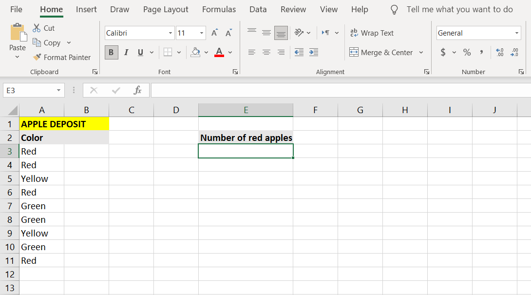
In this example, we have a list of apples and their colors. The goal is to write a formula that will count the number of red apples and then display it in a cell. Using a cell range where apple colors are placed as the range, we will instruct the formula to count only the red ones in that range when using the COUNTIF function.

1. Select the cell where you want to display the result of the count. In this example, we’re going to use cell E3.
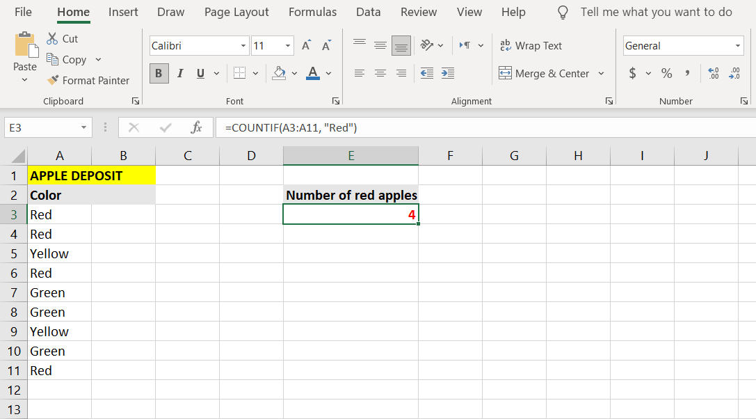
2. Once you have the cell selected, go to the formula bar and enter the formula below:

    =COUNTIF(A3:A11, "Red") 

   Since the target range in this example, where the apple colors are located, is cells A3 to A11, the formula is given A3:A11 in the first part. The second part, which is the criteria, has to specify that the COUNTIF function counts only the red apples. Thence the “Red” in the second part. Remember that you have to put text criteria between quote marks.

3. Press Enter.
4. Excel will now count the number of red apples and display it.

The COUNTIF function allows you to accomplish many wonderful things, especially when used with wildcards and other functions, but it can only consider one condition. In contrast, its relative, the COUNTIFS function, operates on multiple conditions for multiple ranges.

How to Use COUNTIFS in Excel

The COUNTIFS function is basically a more sophisticated version of the COUNTIF function. The main advantage that COUTNIFS holds over COUNTIF is that it supports multiple conditions and ranges.

However, you can also define a single range and a single condition for the COUNTIFS function, making it no practically different from the COUNTIF function.

One important thing that you should understand about the COUNTIFS function before using it is that the COUNTIFS function does not simply sum the results of cells that meet the criteria for each cell range.

In reality, if you have two conditions for two ranges, the cells in the first range are filtered twice: once through the first condition, and then through the second condition. This means that the COUTNIFS function will only return values that meet both conditions, in their given ranges.

You can get a better understanding of what exactly the COUNTIFS function does by studying the example below.

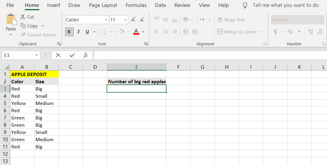
We’ve extended the example from the previous section, and now aside from the color of the apples, there’s a column describing their size as well. The ultimate goal in this example is to count the number of big red apples.

1. Select the cell where you want to display the results. (In this example, we’re going to display the count of big red apples in cell E3.)
2. Go to the formula bar and enter the formula below:

    =COUNTIFS(A3:A11, "Red", B3:B11, "Big") 

   With this, the formula tests the cells from A3 to A11 for the condition “Red”. The cells, which pass the test, are then further tested in range B3 to B11 for the condition “Big”.

3. Press Enter.
4. Excel will now count the number of big red apples.

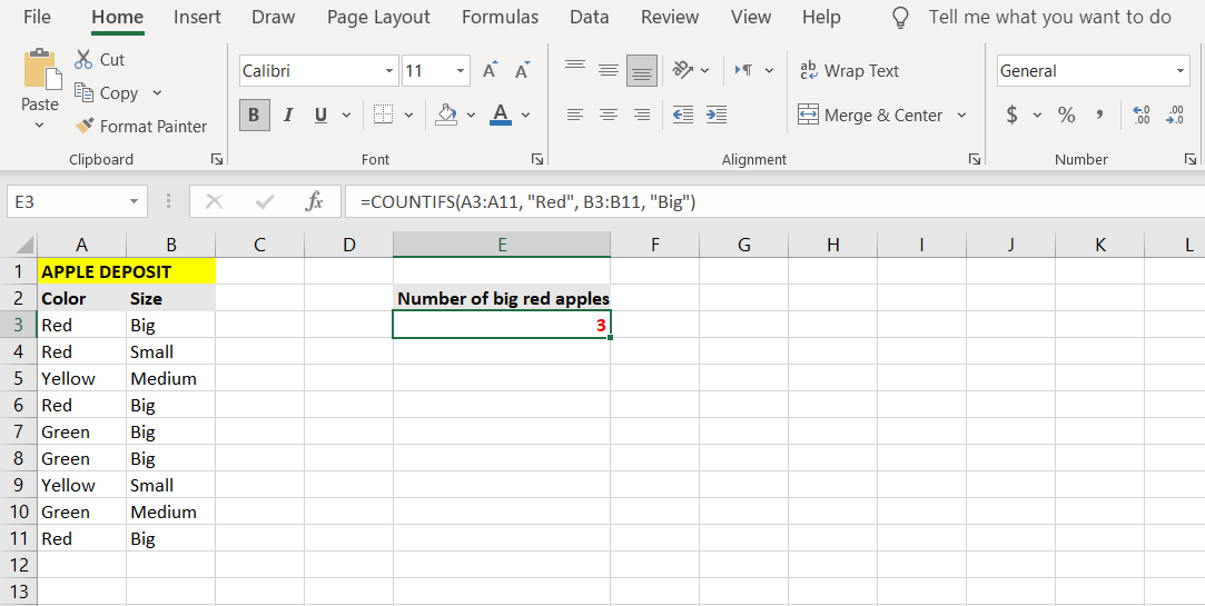
Observe how the formula counts cells that have both the red and the big attribute. The formula takes the cells from A3 to A11 and tests them for the color red. Cells that pass this test, are then again tested for the second condition in the second range, which in this case, is being big.

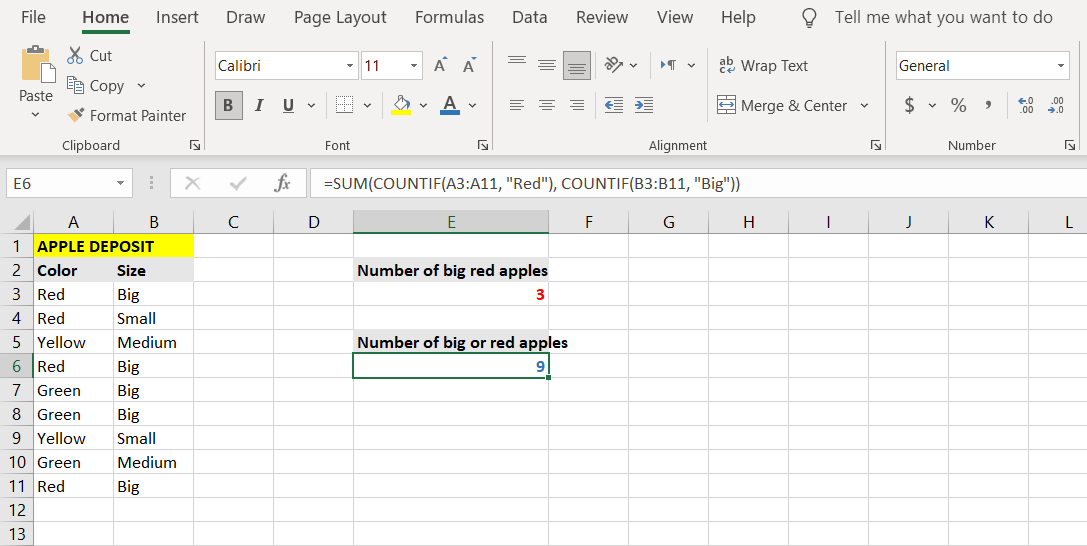
In conclusion, the ranges and conditions after the first range and condition further narrow down the count filter and are not independent of each other. So then the final result of the formula is apples that are red and big. You can count the number of red or big apples by combining the COUNTIF function with the SUM function.

1. Select the cell where you want to display the result of your formula. (In this example, we’re going to use cell E6.)
2. Enter the formula below:

    =SUM(COUNTIF(A3:A11, "Red"), COUNTIF(B3:B11, "Big")) 

   This formula will count the cells containing red apples, then the number of cells containing big apples, and finally, it will sum the two numbers.

3. Press Enter.
4. Excel will now count and display the number of big or red apples.

Count More With Excel

If you have multiplied conditions for a count, or simply too long a list, then counting manually can become very frustrating. With Excel and its COUNTIF and COUNTIFS functions, you can write a formula that will take care of the counting process for you.

The small effort you make to learn this new Excel formula will allow you to gain great benefits in the future. Perhaps combining SUMPRODUCT and COUNTIF will yield some good?

The COUNTIFS function in Excel is one of the best functions to know.

Whether you’re considering a career as a data analyst or just want to hone your expertise in Excel, I highly recommend that you master this function. It is very versatile and has helped me accomplish a wide variety of tasks over the years.

The COUNTIFS function is used to count only the values in a list that meet specified criteria. For example, only count the orders for a specific product, or only count the exam scores where the result was 70 or higher.

In this tutorial, we’ll show you how to use the COUNTIFS function. We’ll also provide a few examples of using COUNTIFS in different scenarios .

We’ll cover:

1. What is the COUNTIFS function and why use it?
2. How to use the COUNTIFS function (step-by-step)
3. Things to consider when using the COUNTIFS function
4. Testing numbers with the COUNTIFS function
5. Testing multiple conditions with COUNTIFS
6. Using cell references with COUNTIFS
7. Combine text and cell references in your criteria
8. COUNTIFS function with date conditions

So: let’s dive into the COUNTIFS function.

1. What is the COUNTIFS function and why use it?

The COUNTIFS function was introduced in 2007 to be the successor to the COUNTIF function in Excel.

The COUNTIF function can count values when a single condition is met. However, COUNTIFS can test a single or multiple conditions. So, it is useful to be aware of the COUNTIF function, but COUNTIFS is far superior.

If you’re using Excel for data analysis, then this function is incredibly useful. Along with sum and average, count is another common requirement when analyzing data.

With the COUNTIFS function, you can count the values that meet any criteria that you specify.

The COUNTIFS function requires only two arguments, but can handle many more optional criteria.

=COUNTIFS(criteria_range1, criteria1, [criteria_range2], [criteria2], …)

Criteria range 1: This is the range that is being tested.

Criteria 1: The criteria to apply to the criteria range. This can be a number, text, a cell reference or another function. We will see some of these examples in this tutorial.

[Criteria range 2, Criteria 2], …: Additional ranges and the criteria to apply to them. Using these extra criteria is optional.

2. How to use the COUNTIFS function (step-by-step)

The examples in this tutorial use the table of data as shown in the following example. You can use this Excel workbook to follow along with the examples.

In this first example, we want to use the COUNTIFS function to count the number of orders from the region Central.

Click in the cell where you would like to return the result, and enter the following formula.

=COUNTIFS($B$2:$B$12,”Central”)

Range B2:B12 has been specified as the criteria range. The criteria “Central” has been typed inside the double quotation marks (“) to denote written text.

The criteria is always written into COUNTIFS inside double quotation marks when text characters are used. When the criteria is a number, cell reference, or a function then the double quotations are not required.

3. Things to consider when using the COUNTIFS function

There are a few things to be aware of when using COUNTIFS.

• When testing multiple criteria, every condition must be met for a value to be counted.
• The number of rows and columns must be the same for each criteria range specified.
• When testing text, COUNTIFS will perform an exact match. However, it is not case-sensitive.
• The ampersand (&) can be used to make criteria from a combination of text and cell references. Examples of this are shown in section seven.
• The asterisk (*) and question mark (?) wildcard characters can be used for partial matches.
• The Tilde (~) character can be used in front of the asterisk or question mark, if you need to count those specific characters.

4. Testing numbers with the COUNTIFS function

The previous example, saw the COUNTIFS function using a text string as its criteria. Let’s now look at an example that tests numeric values.

The following formula returns the number of orders valued at 500 or more.

=COUNTIFS($D$2:$D$12,”>=500”)

In this example, range D2:D12 is specified as the criteria range. The criteria is still entered within double quotation marks, because the “>=” characters are used.

The logical operators “<” for less than and “<>” for not equal to, can also be used when specifying the criteria.

5. Testing multiple conditions with COUNTIFS

Remember, the COUNTIFS function can handle multiple conditions (up to 127 conditions). This makes it superior to the legacy COUNTIF function.

So, let’s combine the two previous examples into one formula. This formula counts the orders that are Central and also greater than or equal to 500.

=COUNTIFS($B$2:$B$12,”Central”,$D$2:$D$12,”>=500”)

Ensure that the number of rows and columns of each criteria range are the same when using multiple conditions in the COUNTIFS function.

6. Using cell references with COUNTIFS

All of the examples so far have demonstrated the criteria being entered directly into the COUNTIFS function.

Formulas can be made more dynamic by referencing other cells that contain the criteria.

In this formula, the criteria for range B2:B12 has been entered into cell F3 and the criteria for range D2:D12 has been entered into cell F4.

=COUNTIFS($B$2:$B$12,F3,$D$2:$D$12,F4)

The formula result will change when the values in cells F3 and F4 are changed.

7. Combine text and cell references in your criteria

Taking the previous example further, entering the logical operators such as “>=” into cell F4 with the value is not ideal. Not all Excel users will be comfortable with this.

The ampersand (&) can be used to combine text and a cell reference together to form criteria.

This formula expands on the previous example by using the ampersand to join the text string “>=” and cell F4.

=COUNTIFS($B$2:$B$12,F3,$D$2:$D$12,”>=”&F4)

Now, users can simply change the text in cell F3 or the number in cell F4 to update the formula criteria.

8. COUNTIFS function with date conditions

Performing analysis on dates is very commonplace. So, let’s look at examples of the COUNTIFS function with date conditions.

The following formula counts the orders since the date entered into cell F3, and for the region entered into cell F4.

=COUNTIFS($A$2:$A$12,”>=”&F3,$B$2:$B$12,F4)

The ampersand was used to join the “>=” operators and the reference to cell F3 like in example 5, as dates are numbers also. However, ensure that the value in cell F3 is recognised as a date.

If you want to enter the date condition directly into the formula instead of using a cell reference, you can enter the date into the criteria like in example 2.

=COUNTIFS($A$2:$A$12,”>=01/11/2020”,$B$2:$B$12,F4)

Final thoughts

Excel formulas are an extremely handy tool for anyone working with data—especially data analysts. For a hands-on introduction to the field of data analytics, try out this free five-day short course. And, for more Excel tutorials, check out the following:

• How to use the SUBTOTAL function in Excel
• How to use the SUMIF function in Excel
• How to use the CONCATENATE function in Excel
• How to use the IFERROR function in Excel

In this tutorial we’re looking at the COUNTIF and COUNTIFS Formulas, and we’ll take a look at a couple of different applications for them.

Plus you can download a practice workbook, you’ll find the file down below.

The COUNTIF/S functions work ALMOST in the same way as the SUMIF/S functions only they’re slightly simpler.  So if you haven’t mastered SUMIF/S yet be sure to check out our SUMIF/S tutorial too.

COUNTIF extends the capabilities of the basic COUNT function by allowing you to tell Excel to only COUNT items that meet a certain criteria.  New in Excel 2007 is the COUNTIFS function, which allows you to stipulate multiple criteria, hence the plural.

Enough explanation, let’s dive into an example as it’s easier to visualise.

COUNTIF Function

The function wizard in Excel describes COUNTIF as:

=COUNTIF(range,criteria)

Looks fairly simple and it is.  Let’s translate it into English now by applying it to an example. Say we wanted to count the number of times Dave appeared in column C of the table below.

Translated our formula would read like this:

=COUNTIF(count the number of cells in column C, that contain 'Dave')

We could even create a table under the data to count the occurrences of each builder:

Our formula in cell C12 would be:

=COUNTIF(C2:C7,"Dave")

While the above formula is good, if we were to copy it to the rest of the summary table (cells C11 to C14) we would have to manually change the cell references and builder’s name to get the correct answers.

To avoid this manual intervention, we can use absolute references, which will speed up the process of copying the formula to the remainder of column C. 

With absolute references our formula would look like this:

=COUNTIF($C$2:$C$7,$B12)

 
The ‘$’ signs tell Excel that we don’t want the reference after the ‘$’ sign to change when we copy the formula.  For example, if we copied the formula into cell C13 it would read:

=COUNTIF($C$2:$C$7,$B13)

In the above formula we can see that the only reference that changed was $B12, which became $B13.

The best way to understand how this works is to try it for yourself. 

Note: I used a basic example to illustrate how to use COUNTIF, but you could also achieve this count by builder using the subtotal tool in the Data tab. 

COUNTIFS Function

The function wizard in Excel describes COUNTIFS as:

=COUNTIFS(critera_range_1,criteria_1,criteria_range_2,criteria_2.....and so on if required)

Extending the previous COUNTIF example above, say we wanted to only summarise the data by builder for jobs in the South region.  We could use the COUNTIFS function, as it allows us to set more than one condition.

Here’s how the formula would be interpreted if we wanted to count the occurrences of Brian in column C, where jobs were in the South region:

=COUNTIFS(count the number of cells in column C if, they contain ‘Brian’ and, if in column B, they are also for the South region)

Note: Excel will only include the cells in column C in the count when both conditions (Brian & South) are met.

Using absolute references, our COUNTIFS formula in Excel cell C20 would read:

=COUNTIFS($C$2:$C$7,$B20,$B$2:$B$7,$B$17)

Try other operators

Just like the IF Statement and SUMIF formula, the COUNTIF and COUNTIFS are based on logic.  This means you can employ different tests other than the text matching (Brian & South) we’ve used above.

Other operators you could use are:

• =             Equal to
• <             Less Than
• >             Greater Than
• <=          Less than or equal to
• >=          Greater than or equal to
• <>          Less than or greater than

For example, if you wanted to count the jobs with an average > $300k the formula would be:

=COUNTIF($E$2:$E$7,">300")

Note: again I’ve used a simple example to illustrate this, but another way to achieve this summary table for each builder by region is to use a Pivot Table.

Want to Learn More Excel Formulas

Why not visit our list of Excel formulas. You’ll find a huge range all explained in plain English, plus PivotTables and other Excel tools and tricks. Enjoy 🙂

Spread the Word

If you found this useful please share it with your friends and colleagues on Google+1, LinkedIn, Facebook and Twitter.

The COUNTIFS function counts cells in a range that meet one or more conditions, referred to as criteria. To apply conditions, the COUNTIFS function supports logical operators (>,<,<>,=) and wildcards (*,?) for partial matching. The COUNTIFS function is a common, widely used function in Excel, and can be used to count cells that contain dates, numbers, and text.

Syntax

The syntax for the COUNTIFS function depends on the criteria being evaluated. Each separate condition will require a range and a criteria. The generic syntax looks like this:

=COUNTIFS(range1,criteria1) // 1 condition
=COUNTIFS(range1,criteria1,range2,criteria2) // 2 conditions

The first two arguments, range1 and criteria1 are required. Range1 is the range to which criteria1 should be applied. Range2 is the range to which criteria2 should be applied. Additional conditions are applied by providing more range and criteria arguments: the third condition is defined by range3 and criteria3, the fourth condition is defined by range4 and criteria4, and so on. When using COUNTIFS, keep the following in mind:

• To be included in the final result, all conditions must be TRUE.
• All ranges must be the same size or COUNTIFS will return a #VALUE! error.
• Criteria should include logical operators (>,<,<>,<=,>=) as needed.
• Each new condition requires a separate range and criteria.

Criteria

The COUNTIFS function supports logical operators (>,<,<>,=) and wildcards (*,?) for partial matching. Because COUNTIFS is in a group of eight functions that split logical criteria into two parts, the syntax is a bit tricky. Each condition requires a separate range and criteria, and operators need to be enclosed in double quotes («»). The table below shows some common examples:

Target	Criteria
Cells greater than 75	«>75»
Cells equal to 100	100 or «100»
Cells less than or equal to 100	«<=100»
Cells equal to «Red»	«red»
Cells not equal to «Red»	«<>red»
Cells that are blank «»	«»
Cells that are not blank	«<>»
Cells that begin with «X»	«x*»
Cells less than A1	«<«&A1
Cells less than today	«<«&TODAY()

Notice the last two examples use concatenation with the ampersand (&) character. When a criteria argument includes a value from another cell, or the result of a formula, logical operators like «<» must be joined with concatenation. This is because Excel needs to evaluate cell references and formulas first to get a value before that value can be joined to an operator.

Basic example

With the example shown, COUNTIFS can be used to count records using 2 criteria as follows:

=COUNTIFS(C5:C14,"red",D5:D14,"tx") // red and TX
=COUNTIFS(C5:C14,"red",F5:F14,">20") // red and >20

Notice the COUNTIFS function is not case-sensitive.

Double quotes («») in criteria

In general, text values need to be enclosed in double quotes, and numbers do not. However, when a logical operator is included with a number, the number and operator must be enclosed in quotes as shown below:

=COUNTIFS(A1:A10,100) // count equal to 100
=COUNTIFS(A1:A10,">50") // count greater than 50
=COUNTIFS(A1:A10,"jim") // count equal to "jim"

Note: showing one condition only for simplicity. Additional conditions must follow the same rules.

Value from another cell

When using a value from another cell in a condition, the cell reference must be concatenated to an operator when used. In the example below, COUNTIFS will count the values in A1:A10 that are less than the value in cell B1. Notice the less than operator (which is text) is enclosed in quotes, but the cell reference is not:

=COUNTIFS(A1:A10,"<"&B1) // count cells less than  B1

Note: COUNTIFS is one of several functions that split conditions into two parts: range + criteria. This causes some inconsistencies with respect to other formulas and functions.

Not equal to

To construct «not equal to» criteria, use the «<>» operator surrounded by double quotes («»). For example, the formula below will count cells not equal to «red» in the range A1:A10:

=COUNTIFS(A1:A10,"<>red") // not "red"

Blank cells

COUNTIFS can count cells that are blank or not blank. The formulas below count blank and not blank cells in the range A1:A10:

=COUNTIFS(A1:A10,"<>") // not blank
=COUNTIFS(A1:A10,"") // blank

Dates

The easiest way to use COUNTIFS with dates is to refer to a valid date in another cell with a cell reference. For example, to count cells in A1:A10 that contain a date greater than a date in B1, you can use a formula like this:

=COUNTIFS(A1:A10, ">"&B1) // count dates greater than A1

Notice we concatenate the «>» operator to the date in B1, but and are no quotes around the cell reference.

The safest way to hardcode a date into COUNTIFS is with the DATE function. This guarantees Excel will understand the date. To count cells in A1:A10 that contain a date less than September 1, 2020, you can use:

=COUNTIFS(A1:A10,"<"&DATE(2020,9,1)) // dates less than 1-Sep-2020

Wildcards

The wildcard characters question mark (?), asterisk(*), or tilde (~) can be used in criteria. A question mark (?) matches any one character, and an asterisk (*) matches zero or more characters of any kind. For example, to count cells in A1:A5 that contain the text «apple» anywhere, you can use a formula like this:

=COUNTIFS(A1:A5,"*apple*") // count cells that contain "apple"

The tilde (~) is an escape character to allow you to find literal wildcards. For example, to count a literal question mark (?), asterisk(*), or tilde (~), add a tilde in front of the wildcard (i.e. ~?, ~*, ~~).

OR logic

The COUNTIFS function is designed to apply multiple criteria, but conditions are applied with AND logic. This means if you try to count cells that contain «red» or «blue» in the same range, the result will be zero (0). However, to count cells with OR logic, you can use an array constant and the SUM function like this:

=SUM(COUNTIFS(range,{"red","blue"})) // red or blue

The formula above will count cells in range that contain «red» or «blue». Briefly, COUNTIFS returns two counts in an array (one for «red» and one for «blue») and the SUM function returns the sum as a final result. For more information, see this example.

Limitations

The COUNTIFS function has some limitations you should be aware of:

• Conditions in COUNTIFS are joined by AND logic. In other words, all conditions must be TRUE in order for a cell to be included in a count. The workaround above can be used in simple situations.
• The COUNTIFS function requires actual ranges for all range arguments; you can’t use an array. This means you can’t alter values that appear in a range argument before applying criteria.
• COUNTIFS is not case-sensitive. To count values based on a case-sensitive condition, you can use a formula based on the SUMPRODUCT function with the EXACT function.
• COUNTIFS has some other quirks, which are detailed in this article.

The most common way to work around the limitations above is to use the SUMPRODUCT function. In the current version of Excel, another option is to use the newer BYROW and BYCOL functions.

Notes

• Multiple conditions are applied with AND logic, i.e. condition 1 AND condition 2, etc.
• All ranges must be the same size. If you supply ranges that don’t match, you’ll get a #VALUE error.
• Non-numeric criteria must be enclosed in double quotes (i.e. «<100»,  «>32», «TX»).
• The wildcard characters ? and * can be used in criteria. A question mark matches any one character and an asterisk matches any sequence of characters.
• To match a literal question mark(?) or asterisk (*), use a tilde (~) like (~?, ~*).