Count with if condition in excel

To count numbers or dates that meet a single condition (such as equal to, greater than, less than, greater than or equal to, or less than or equal to), use the COUNTIF function. To count numbers or dates that fall within a range (such as greater than 9000 and at the same time less than 22500), you can use the COUNTIFS function. Alternately, you can use SUMPRODUCT too.

Example

Note: You’ll need to adjust these cell formula references outlined here based on where and how you copy these examples into the Excel sheet.

1	A	B
2	Salesperson	Invoice
3	Buchanan	15,000
4	Buchanan	9,000
5	Suyama	8,000
6	Suyma	20,000
7	Buchanan	5,000
8	Dodsworth	22,500
9	Formula	Description (Result)
10	=COUNTIF(B2:B7,»>9000″)	The COUNTIF function counts the number of cells in the range B2:B7 that contain numbers greater than 9000 (4)
11	=COUNTIF(B2:B7,»<=9000″)	The COUNTIF function counts the number of cells in the range B2:B7 that contain numbers less than 9000 (4)
12	=COUNTIFS(B2:B7,»>=9000″,B2:B7,»<=22500″)	The COUNTIFS function (available in Excel 2007 and later) counts the number of cells in the range B2:B7 greater than or equal to 9000 and are less than or equal to 22500 (4)
13	=SUMPRODUCT((B2:B7>=9000)*(B2:B7<=22500))	The SUMPRODUCT function counts the number of cells in the range B2:B7 that contain numbers greater than or equal to 9000 and less than or equal to 22500 (4). You can use this function in Excel 2003 and earlier, where COUNTIFS is not available.
14	Date
15	3/11/2011
16	1/1/2010
17	12/31/2010
18	6/30/2010
19	Formula	Description (Result)
20	=COUNTIF(B14:B17,»>3/1/2010″)	Counts the number of cells in the range B14:B17 with a data greater than 3/1/2010 (3)
21	=COUNTIF(B14:B17,»12/31/2010″)	Counts the number of cells in the range B14:B17 equal to 12/31/2010 (1). The equal sign is not needed in the criteria, so it is not included here (the formula will work with an equal sign if you do include it («=12/31/2010»).
22	=COUNTIFS(B14:B17,»>=1/1/2010″,B14:B17,»<=12/31/2010″)	Counts the number of cells in the range B14:B17 that are between (inclusive) 1/1/2010 and 12/31/2010 (3).
23	=SUMPRODUCT((B14:B17>=DATEVALUE(«1/1/2010»))*(B14:B17<=DATEVALUE(«12/31/2010»)))	Counts the number of cells in the range B14:B17 that are between (inclusive) 1/1/2010 and 12/31/2010 (3). This example serves as a substitute for the COUNTIFS function that was introduced in Excel 2007. The DATEVALUE function converts the dates to a numeric value, which the SUMPRODUCT function can then work with.

The COUNTIFS function is designed to count the number of cells from a range that satisfy one or more criteria, and returns the corresponding numeric value. Unlike the COUNTIF function, which takes only one argument with a data selection criterion, the function in question allows you to specify up to 127 criteria.



Examples of using the COUNTIFS function in Excel

With the COUNTIFS function, you can calculate the number of cells that meet the criteria applicable to a column with numeric values. For example, cells A1:A9 contain a number series from 1 to 9. Function = COUNTIFS(A1:A9,»>2″A1:A9,»<6″) returns 3 because there are 3 numbers between numbers 2 and 6 ( 3, 4 and 5). Also, data selection criteria can be applied to other columns of the table.



How to calculate the number of positions in the price list by the condition?

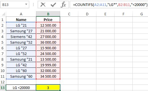
Example 1. Determine the number of LG-made TVs in the data table, the value of which does not exceed 20,000.

View source table:

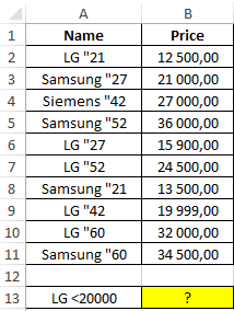
To calculate the number of LG TVs, the cost of which does not exceed 20,000, we use the following formula:

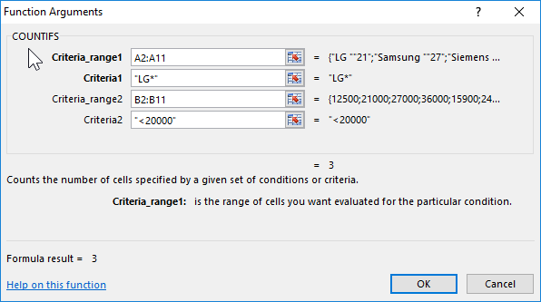
Argument Description:

• A2:A11 — the range of the first condition, the cells of which store text data with the company name and the diagonal value;
• «LG *» — search condition with the wildcard «*» (any number of characters after «LG»;
• B2:B11 — the range of the second condition, containing the value of the goods;
• «<20000» is the second search term (price is less than 20,000).

Result of calculations:

How to calculate the share of a group of products in the price list?

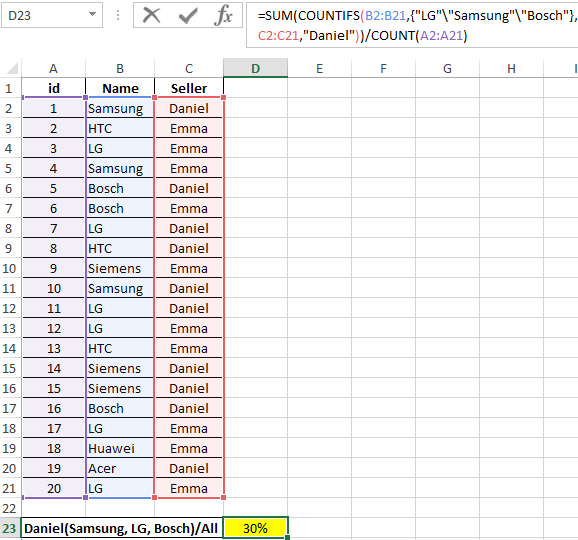
Example 2. The table contains data on purchases in the online home appliances store for a certain period of time. Determine the ratio of LG, Samsung and Bosch products sold by the seller with the last name Ivanov to the total quantity of goods sold by all sellers.

View source table:

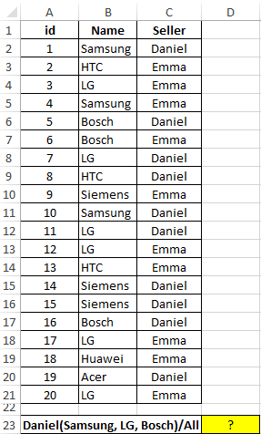
To obtain the desired value, we use the formula:

To search for several values at once in the data vector (column B: B), the argument of condition1 was the array constant {«LG»,»Samsung»,»Bosch»} therefore, the formula must be executed as an array formula. The SUM function counts the number of elements contained in the array of values returned by the COUNTIFS function. The COUNT function returns the number of non-empty cells in the A2: A21 range, that is, the number of rows in the table. The ratio of the obtained values is the desired value.

As a result of the calculations we get:

How to count the number of cells for several conditions in Excel?

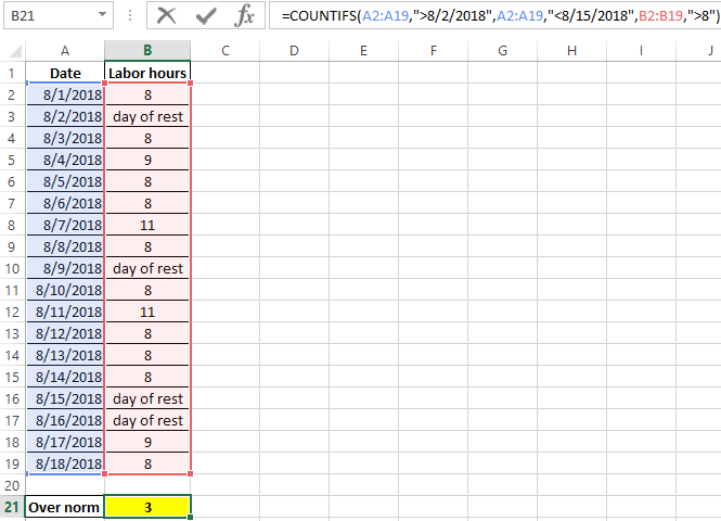
Example 3. The table shows data on the number of hours worked by an employee over a period of time. Determine how many times an employee has worked in excess of the norm (more than 8 hours) in the period from 08/03/2018 through 08/14/2018.

View of data table:

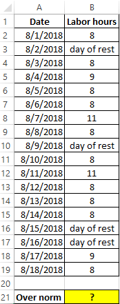
For calculations, use the following formula:

The first two verification conditions are dates that are automatically converted to an Excel time code (numeric value), and then the verification operation is performed. The last (third) criterion — the number of working hours is more than 8.

As a result of calculations, we obtain the following value:

Features of using the COUNTIFS function in Excel

The function has the following syntax entry:

=COUNTIFS(Criteria_range1,Criteria1,[condition_ range2,condition2],…)

Argument Description:

• Criteria_range1 is a required argument that accepts a reference to a range of cells for which the criterion specified in the second argument will be applied to the data contained;
• Criteria1 is a required argument that accepts a condition for selecting data from a range of cells specified as a range_condition1. This argument takes numbers, data of a reference type, text strings containing logical expressions. For example, from the table containing the fields “Name”, “Cost”, “Screen diagonal” you need to select devices whose price does not exceed $ 1,000, the manufacturer is Samsung, and the diagonal is 5 inches. As conditions, you can specify “Samsung *” (the wildcard “*” replaces any number of characters), “> 1000” (price over 1000, the expression must be specified in quotes), 5 (exact numerical value, quotes are optional);
• [range_condition2; condition2]; … — a pair of subsequent arguments of the function in question, the meaning of which corresponds to the arguments range_condition1 and condition1, respectively. Up to 127 ranges and conditions for selecting values can be specified.

Download examples COUNTIFS function calculates in Excel

Notes:

1. In the second and subsequent condition ranges ([condition_range2], [condition_range3], etc.), the number of cells must correspond to their number in the range specified by the condition_range1 argument. Otherwise, the COUNTIFS function will return the error code #VALUE !.
2. The function in question checks all the conditions listed as condition1, [condition2], and so on, for each row. If all conditions are met, the total amount returned by COUNTIFS is increased by one.
3. If the condition N argument was passed to a reference to an empty cell, the conversion of the empty value to a numeric 0 (zero) is performed.
4. When using textual conditions, you can set inaccurate filters with the wildcard characters «*» and «?».

The COUNTIF function counts cells in a range that meet a given condition, referred to as criteria. COUNTIF is a common, widely used function in Excel, and can be used to count cells that contain dates, numbers, and text. Note that COUNTIF can only apply a single condition. To count cells with multiple criteria, see the COUNTIFS function.

Syntax

The generic syntax for COUNTIF looks like this:

=COUNTIF(range,criteria)

The COUNTIF function takes two arguments, range and criteria. Range is the range of cells to apply a condition to. Criteria is the condition to apply, along with any logical operators that are needed.

Applying criteria

The COUNTIF function supports logical operators (>,<,<>,<=,>=) and wildcards (*,?) for partial matching. The tricky part about using the COUNTIF function is the syntax used to apply criteria. COUNTIFS is in a group of eight functions that split logical criteria into two parts, range and criteria. Because of this design, each condition requires a separate range and criteria argument, and operators in the criteria must be enclosed in double quotes («»). The table below shows examples of the syntax needed for common criteria:

Target	Criteria
Cells greater than 75	«>75»
Cells equal to 100	100 or «100»
Cells less than or equal to 100	«<=100»
Cells equal to «Red»	«red»
Cells not equal to «Red»	«<>red»
Cells that are blank «»	«»
Cells that are not blank	«<>»
Cells that begin with «X»	«x*»
Cells less than A1	«<«&A1
Cells less than today	«<«&TODAY()

Notice the last two examples involve concatenation with the ampersand (&) character.  Any time you are using a value from another cell, or using the result of a formula in criteria with a logical operator like «<«, you will need to concatenate. This is because Excel needs to evaluate cell references and formulas first to get a value, before that value can be joined to an operator.

Basic example

In the worksheet shown above, the following formulas are used in cells G5, G6, and G7:

=COUNTIF(D5:D12,">100") // count sales over 100
=COUNTIF(B5:B12,"jim") // count name = "jim"
=COUNTIF(C5:C12,"ca") // count state = "ca"

Notice COUNTIF is not case-sensitive, «CA» and «ca» are treated the same.

Double quotes («») in criteria

In general, text values need to be enclosed in double quotes («»), and numbers do not. However, when a logical operator is included with a number, the number and operator must be enclosed in quotes, as seen in the second example below:

=COUNTIF(A1:A10,100) // count cells equal to 100
=COUNTIF(A1:A10,">32") // count cells greater than 32
=COUNTIF(A1:A10,"jim") // count cells equal to "jim"

Value from another cell

A value from another cell can be included in criteria using concatenation. In the example below, COUNTIF will return the count of values in A1:A10 that are less than the value in cell B1. Notice the less than operator (which is text) is enclosed in quotes.

=COUNTIF(A1:A10,"<"&B1) // count cells less than  B1

Not equal to

To construct «not equal to» criteria, use the «<>» operator surrounded by double quotes («»). For example, the formula below will count cells not equal to «red» in the range A1:A10:

=COUNTIF(A1:A10,"<>red") // not "red"

Blank cells

COUNTIF can count cells that are blank or not blank. The formulas below count blank and not blank cells in the range A1:A10:

=COUNTIF(A1:A10,"<>") // not blank
=COUNTIF(A1:A10,"") // blank

Note: be aware that COUNTIF treats formulas that return an empty string («») as not blank. See this example for some workarounds to this problem.

Dates

The easiest way to use COUNTIF with dates is to refer to a valid date in another cell with a cell reference. For example, to count cells in A1:A10 that contain a date greater than the date in B1, you can use a formula like this:

=COUNTIF(A1:A10, ">"&B1) // count dates greater than A1

Notice we must concatenate an operator to the date in B1. To use more advanced date criteria (i.e. all dates in a given month, or all dates between two dates) you’ll want to switch to the COUNTIFS function, which can handle multiple criteria.

The safest way to hardcode a date into COUNTIF is to use the DATE function. This ensures Excel will understand the date. To count cells in A1:A10 that contain a date less than April 1, 2020, you can use a formula like this

=COUNTIF(A1:A10,"<"&DATE(2020,4,1)) // dates less than 1-Apr-2020

Wildcards

The wildcard characters question mark (?), asterisk(*), or tilde (~) can be used in criteria. A question mark (?) matches any one character and an asterisk (*) matches zero or more characters of any kind. For example, to count cells in A1:A5 that contain the text «apple» anywhere, you can use a formula like this:

=COUNTIF(A1:A5,"*apple*") // cells that contain "apple"

To count cells in A1:A5 that contain any 3 text characters, you can use:

=COUNTIF(A1:A5,"???") // cells that contain any 3 characters

The tilde (~) is an escape character to match literal wildcards. For example, to count a literal question mark (?), asterisk(*), or tilde (~), add a tilde in front of the wildcard (i.e. ~?, ~*, ~~).

OR logic

The COUNTIF function is designed to apply just one condition. However, to count cells that contain «this OR that», you can use an array constant and the SUM function like this:

=SUM(COUNTIF(range,{"red","blue"})) // red or blue

The formula above will count cells in range that contain «red» or «blue». Essentially, COUNTIF returns two counts in an array (one for «red» and one for «blue») and the SUM function returns the sum. For more information, see this example.

Limitations

The COUNTIF function has some limitations you should be aware of:

• COUNTIF only supports a single condition. If you need to count cells using multiple criteria, use the COUNTIFS function.
• COUNTIF requires an actual range for the range argument; you can’t provide an array. This means you can’t alter values in range before applying criteria.
• COUNTIF is not case-sensitive. Use the EXACT function for case-sensitive counts.
• COUNTIFS has other quirks explained in this article.

The most common way to work around the limitations above is to use the SUMPRODUCT function. In the current version of Excel, another option is to use the newer BYROW and BYCOL functions.

Notes

• Text strings in criteria must be enclosed in double quotes («»), i.e. «apple», «>32», «app*»
• Cell references in criteria are not enclosed in quotes, i.e. «<«&A1
• The wildcard characters ? and * can be used in criteria. A question mark matches any one character and an asterisk matches any sequence of characters (zero or more).
• To match a literal question mark(?) or asterisk (*), use a tilde (~) like (~?, ~*).
• COUNTIF requires a range, you can’t substitute an array.
• COUNTIF returns incorrect results when used to match strings longer than 255 characters.
• COUNTIF will return a #VALUE error when referencing another workbook that is closed.

Excel has many functions where a user needs to specify a single or multiple criteria to get the result. For example, if you want to count cells based on multiple criteria, you can use the COUNTIF or COUNTIFS functions in Excel.

This tutorial covers various ways of using a single or multiple criteria in COUNTIF and COUNTIFS function in Excel.

While I will primarily be focussing on COUNTIF and COUNTIFS functions in this tutorial, all these examples can also be used in other Excel functions that take multiple criteria as inputs (such as SUMIF, SUMIFS, AVERAGEIF, and AVERAGEIFS).

An Introduction to Excel COUNTIF and COUNTIFS Functions

Let’s first get a grip on using COUNTIF and COUNTIFS functions in Excel.

Excel COUNTIF Function (takes Single Criteria)

Excel COUNTIF function is best suited for situations when you want to count cells based on a single criterion. If you want to count based on multiple criteria, use COUNTIFS function.

Syntax

=COUNTIF(range, criteria)

Input Arguments

• range –  the range of cells which you want to count.
• criteria – the criteria that must be evaluated against the range of cells for a cell to be counted.

Excel COUNTIFS Function (takes Multiple Criteria)

Excel COUNTIFS function is best suited for situations when you want to count cells based on multiple criteria.

Syntax

=COUNTIFS(criteria_range1, criteria1, [criteria_range2, criteria2]…)

Input Arguments

• criteria_range1 – The range of cells for which you want to evaluate against criteria1.
• criteria1 – the criteria which you want to evaluate for criteria_range1 to determine which cells to count.
• [criteria_range2] – The range of cells for which you want to evaluate against criteria2.
• [criteria2] – the criteria which you want to evaluate for criteria_range2 to determine which cells to count.

Now let’s have a look at some examples of using multiple criteria in COUNTIF functions in Excel.

Using NUMBER Criteria in Excel COUNTIF Functions

#1 Count Cells when Criteria is EQUAL to a Value

To get the count of cells where the criteria argument is equal to a specified value, you can either directly enter the criteria or use the cell reference that contains the criteria.

Below is an example where we count the cells that contain the number 9 (which means that the criteria argument is equal to 9). Here is the formula:

=COUNTIF($B$2:$B$11,D3)

In the above example (in the pic), the criteria is in cell D3. You can also enter the criteria directly into the formula. For example, you can also use:

=COUNTIF($B$2:$B$11,9)

#2 Count Cells when Criteria is GREATER THAN a Value

To get the count of cells with a value greater than a specified value, we use the greater than operator (“>”). We could either use it directly in the formula or use a cell reference that has the criteria.

Whenever we use an operator in criteria in Excel, we need to put it within double quotes. For example, if the criteria is greater than 10, then we need to enter “>10” as the criteria (see pic below):

Here is the formula:

=COUNTIF($B$2:$B$11,”>10″)

You can also have the criteria in a cell and use the cell reference as the criteria. In this case, you need NOT put the criteria in double quotes:

=COUNTIF($B$2:$B$11,D3)

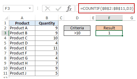
There could also be a case when you want the criteria to be in a cell, but don’t want it with the operator. For example, you may want the cell D3 to have the number 10 and not >10.

In that case, you need to create a criteria argument which is a combination of operator and cell reference (see pic below):

=COUNTIF($B$2:$B$11,”>”&D3)

NOTE: When you combine an operator and a cell reference, the operator is always in double quotes. The operator and cell reference are joined by an ampersand (&).

#3 Count Cells when Criteria is LESS THAN a Value

To get the count of cells with a value less than a specified value, we use the less than operator (“<“). We could either use it directly in the formula or use a cell reference that has the criteria.

Whenever we use an operator in criteria in Excel, we need to put it within double quotes. For example, if the criterion is that the number should be less than 5, then we need to enter “<5” as the criteria (see pic below):

=COUNTIF($B$2:$B$11,”<5″)

You can also have the criteria in a cell and use the cell reference as the criteria. In this case, you need NOT put the criteria in double quotes (see pic below):

=COUNTIF($B$2:$B$11,D3)

Also, there could be a case when you want the criteria to be in a cell, but don’t want it with the operator. For example, you may want the cell D3 to have the number 5 and not <5.

In that case, you need to create a criteria argument which is a combination of operator and cell reference:

=COUNTIF($B$2:$B$11,”<“&D3)

NOTE: When you combine an operator and a cell reference, the operator is always in double quotes. The operator and cell reference are joined by an ampersand (&).

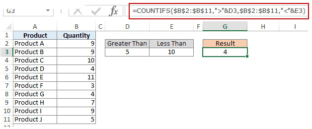
#4 Count Cells with Multiple Criteria – Between Two Values

To get a count of values between two values, we need to use multiple criteria in the COUNTIF function.

Here are two methods of doing this:

METHOD 1: Using COUNTIFS function

COUNTIFS function can handle multiple criteria as arguments and counts the cells only when all the criteria are TRUE. To count cells with values between two specified values (say 5 and 10), we can use the following COUNTIFS function:

=COUNTIFS($B$2:$B$11,”>5″,$B$2:$B$11,”<10″)

NOTE: The above formula does not count cells that contain 5 or 10. If you want to include these cells, use greater than equal to (>=) and less than equal to (<=) operators. Here is the formula:

=COUNTIFS($B$2:$B$11,”>=5″,$B$2:$B$11,”<=10″) 

You can also have these criteria in cells and use the cell reference as the criteria. In this case, you need NOT put the criteria in double quotes (see pic below):

You can also use a combination of cells references and operators (where the operator is entered directly in the formula). When you combine an operator and a cell reference, the operator is always in double quotes. The operator and cell reference are joined by an ampersand (&).

METHOD 2: Using two COUNTIF functions

If you have multiple criteria, you can either use COUNTIFS or create a combination of COUNTIF functions. The formula below would also do the same thing:

=COUNTIF($B$2:$B$11,”>5″)-COUNTIF($B$2:$B$11,”>10″)

In the above formula, we first find the number of cells that have a value greater than 5 and we subtract the count of cells with a value greater than 10. This would give us the result as 5 (which is the number of cells that have values more than 5 and less than equal to 10).

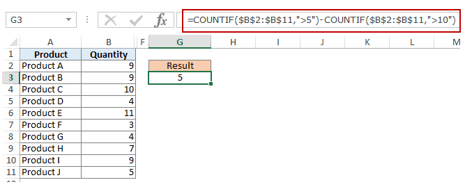
If you want the formula to include both 5 and 10, use the following formula instead:

=COUNTIF($B$2:$B$11,”>=5″)-COUNTIF($B$2:$B$11,”>10″)

If you want the formula to exclude both ‘5’ and ’10’ from the counting, use the following formula:

=COUNTIF($B$2:$B$11,”>=5″)-COUNTIF($B$2:$B$11,”>10″)-COUNTIF($B$2:$B$11,10)

You can have these criteria in cells and use the cells references, or you can use a combination of operators and cells references.

Using TEXT Criteria in Excel Functions

#1 Count Cells when Criteria is EQUAL to a Specified text

To count cells that contain an exact match of the specified text, we can simply use that text as the criteria. For example, in the dataset (shown below in the pic), if I want to count all the cells with the name Joe in it, I can use the below formula:

=COUNTIF($B$2:$B$11,”Joe”)

Since this is a text string, I need to put the text criteria in double quotes.

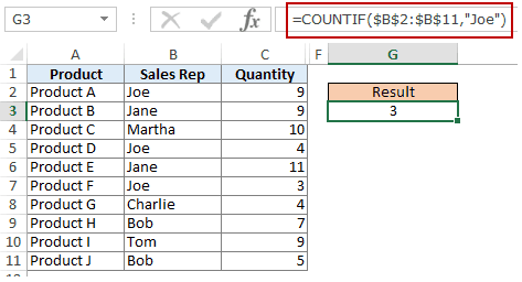
You can also have the criteria in a cell and then use that cell reference (as shown below):

=COUNTIF($B$2:$B$11,E3)

NOTE: You can get wrong results if there are leading/trailing spaces in the criteria or criteria range. Make sure you clean the data before using these formulas.

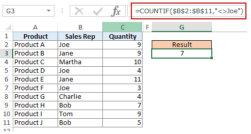
#2 Count Cells when Criteria is NOT EQUAL to a Specified text

Similar to what we saw in the above example, you can also count cells that do not contain a specified text. To do this, we need to use the not equal to operator (<>).

Suppose you want to count all the cells that do not contain the name JOE, here is the formula that will do it:

=COUNTIF($B$2:$B$11,”<>Joe”)

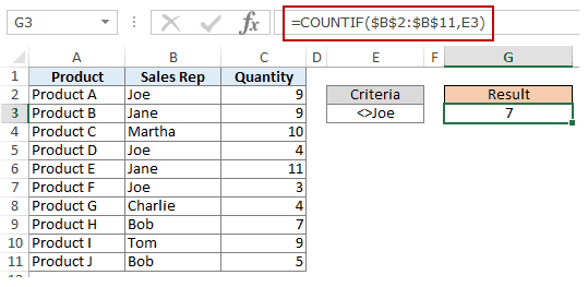
You can also have the criteria in a cell and use the cell reference as the criteria. In this case, you need NOT put the criteria in double quotes (see pic below):

=COUNTIF($B$2:$B$11,E3)

There could also be a case when you want the criteria to be in a cell but don’t want it with the operator. For example, you may want the cell D3 to have the name Joe and not <>Joe.

In that case, you need to create a criteria argument which is a combination of operator and cell reference (see pic below):

=COUNTIF($B$2:$B$11,”<>”&E3)

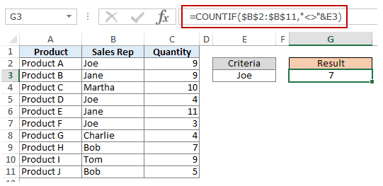
When you combine an operator and a cell reference, the operator is always in double quotes. The operator and cell reference are joined by an ampersand (&).

Using DATE Criteria in Excel COUNTIF and COUNTIFS Functions

Excel store date and time as numbers. So we can use it the same way we use numbers.

#1 Count Cells when Criteria is EQUAL to a Specified Date

To get the count of cells that contain the specified date, we would use the equal to operator (=) along with the date.

To use the date, I recommend using the DATE function, as it gets rid of any possibility of error in the date value. So, for example, if I want to use the date September 1, 2015, I can use the DATE function as shown below:

=DATE(2015,9,1)

This formula would return the same date despite regional differences. For example, 01-09-2015 would be September 1, 2015 according to the  US date syntax and January 09, 2015 according to the UK date syntax. However, this formula would always return September 1, 2105.

Here is the formula to count the number of cells that contain the date 02-09-2015:

=COUNTIF($A$2:$A$11,DATE(2015,9,2))

#2 Count Cells when Criteria is BEFORE or AFTER to a Specified Date

To count cells that contain date before or after a specified date, we can use the less than/greater than operators.

For example, if I want to count all the cells that contain a date that is after September 02, 2015, I can use the formula:

=COUNTIF($A$2:$A$11,”>”&DATE(2015,9,2))

Similarly, you can also count the number of cells before a specified date. If you want to include a date in the counting, use and ‘equal to’ operator along with ‘greater than/less than’ operator.

You can also use a cell reference that contains a date. In this case, you need to combine the operator (within double quotes) with the date using an ampersand (&).

See example below:

=COUNTIF($A$2:$A$11,”>”&F3)

#3 Count Cells with Multiple Criteria – Between Two Dates

To get a count of values between two values, we need to use multiple criteria in the COUNTIF function.

We can do this using two methods – One single COUNTIFS function or two COUNTIF functions.

METHOD 1: Using COUNTIFS function

COUNTIFS function can take multiple criteria as the arguments and counts the cells only when all the criteria are TRUE. To count cells with values between two specified dates (say September 2 and September 7), we can use the following COUNTIFS function:

=COUNTIFS($A$2:$A$11,”>”&DATE(2015,9,2),$A$2:$A$11,”<“&DATE(2015,9,7))

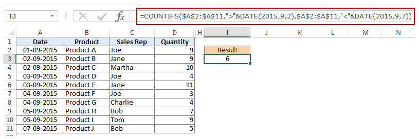
The above formula does not count cells that contain the specified dates. If you want to include these dates as well, use greater than equal to (>=) and less than equal to (<=) operators. Here is the formula:

=COUNTIFS($A$2:$A$11,”>=”&DATE(2015,9,2),$A$2:$A$11,”<=”&DATE(2015,9,7))

You can also have the dates in a cell and use the cell reference as the criteria. In this case, you can not have the operator with the date in the cells. You need to manually add operators in the formula (in double quotes) and add cell reference using an ampersand (&). See the pic below:

=COUNTIFS($A$2:$A$11,”>”&F3,$A$2:$A$11,”<“&G3)

METHOD 2: Using COUNTIF functions

If you have multiple criteria, you can either use one COUNTIFS function or create a combination of two COUNTIF functions. The formula below would also do the trick:

=COUNTIF($A$2:$A$11,”>”&DATE(2015,9,2))-COUNTIF($A$2:$A$11,”>”&DATE(2015,9,7))

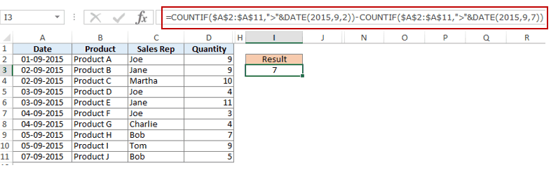
In the above formula, we first find the number of cells that have a date after September 2 and we subtract the count of cells with dates after September 7. This would give us the result as 7 (which is the number of cells that have dates after September 2 and on or before September 7).

If you don’t want the formula to count both September 2 and September 7, use the following formula instead:

=COUNTIF($A$2:$A$11,”>=”&DATE(2015,9,2))-COUNTIF($A$2:$A$11,”>”&DATE(2015,9,7))

If you want to exclude both the dates from counting, use the following formula:

=COUNTIF($A$2:$A$11,”>”&DATE(2015,9,2))-COUNTIF($A$2:$A$11,”>”&DATE(2015,9,7)-COUNTIF($A$2:$A$11,DATE(2015,9,7)))

Also, you can have the criteria dates in cells and use the cells references (along with operators in double quotes joined using ampersand).

Using WILDCARD CHARACTERS in Criteria in COUNTIF & COUNTIFS Functions

There are three wildcard characters in Excel:

1. * (asterisk) – It represents any number of characters. For example, ex* could mean excel, excels, example, expert, etc.
2. ? (question mark) – It represents one single character. For example, Tr?mp could mean Trump or Tramp.
3. ~ (tilde) – It is used to identify a wildcard character (~, *, ?) in the text.

You can use COUNTIF function with wildcard characters to count cells when other inbuilt count function fails. For example, suppose you have a data set as shown below:

Now let’s take various examples:

#1 Count Cells that contain Text

To count cells with text in it, we can use the wildcard character * (asterisk). Since asterisk represents any number of characters, it would count all cells that have any text in it. Here is the formula:

=COUNTIFS($C$2:$C$11,”*”)

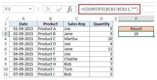
Note: The formula above ignores cells that contain numbers, blank cells, and logical values, but would count the cells contain an apostrophe (and hence appear blank) or cells that contain empty string (=””) which may have been returned as a part of a formula.

Here is a detailed tutorial on handling cases where there is an empty string or apostrophe.

Here is a detailed tutorial on handling cases where there are empty strings or apostrophes.

Below is a video that explains different scenarios of counting cells with text in it.

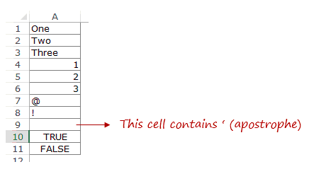
#2 Count Non-blank Cells

If you are thinking of using COUNTA function, think again.

Try it and it might fail you. COUNTA will also count a cell that contains an empty string (often returned by formulas as =”” or when people enter only an apostrophe in a cell). Cells that contain empty strings look blank but are not, and thus counted by the COUNTA function.

COUNTA will also count a cell that contains an empty string (often returned by formulas as =”” or when people enter only an apostrophe in a cell). Cells that contain empty strings look blank but are not, and thus counted by the COUNTA function.

So if you use the formula =COUNTA(A1:A11), it returns 11, while it should return 10.

Here is the fix:

=COUNTIF($A$1:$A$11,”?*”)+COUNT($A$1:$A$11)+SUMPRODUCT(–ISLOGICAL($A$1:$A$11))

Let’s understand this formula by breaking it down:

#3 Count Cells that contain specific text

Let’s say we want to count all the cells where the sales rep name begins with J. This can easily be achieved by using a wildcard character in COUNTIF function. Here is the formula:

=COUNTIFS($C$2:$C$11,”J*”) 

The criteria J* specifies that the text in a cell should begin with J and can contain any number of characters.

If you want to count cells that contain the alphabet anywhere in the text, flank it with an asterisk on both sides. For example, if you want to count cells that contain the alphabet “a” in it, use *a* as the criteria.

This article is unusually long compared to my other articles. Hope you have enjoyed it. Let me know your thoughts by leaving a comment.

You May Also Find the following Excel tutorials useful:

• Count the number of words in Excel.
• Count Cells Based on Background Color in Excel.
• How to Sum a Column in Excel (5 Really Easy Ways)

Return to Excel Formulas List

Download Example Workbook

Download the example workbook

This tutorial demonstrates how to “count if” with multiple criteria using the COUNTIFS Function in Excel and Google Sheets. If your version of Excel does not support COUNTIFS, we also demonstrate how to use the SUMPRODUCT function instead.

COUNTIFS Function

The COUNTIFS Function allows you to count values that meet multiple criteria. The basic formula structure is:

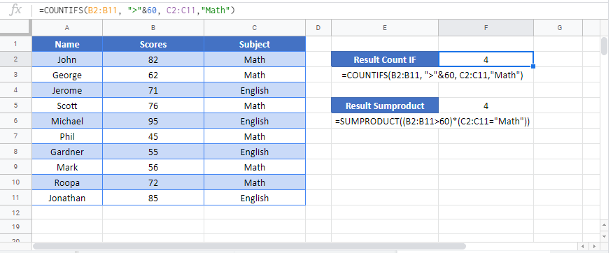
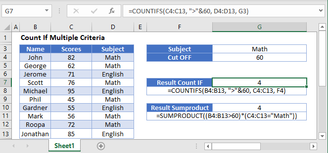
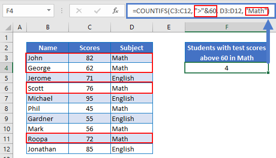
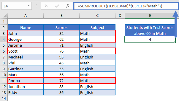
=COUNTIFS(Range 1, Condition 1, Range 2, Condition 2)

Let’s look at an example. Below you will see a list containing grades for students in English and Math. Let’s count all students with test scores above 60 in Math.

=COUNTIFS(C3:C12, ">"&60, D3:D12, "Math")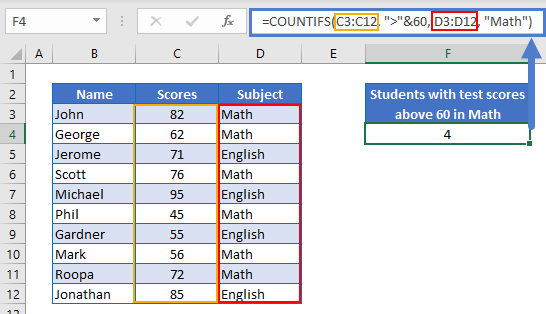

In this case, we are testing two criteria:

1. If the Test Scores are greater than 60 (Range B2:B11)
2. If the Subject is “Math” (Range is C2:C11)

Below, you can see that there are 4 students who scored above 60 in Math:

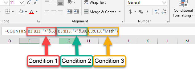
You can test additional conditions by adding another range and criteria.  For example, if you wanted to count the number of students who scored between 60 and 80 in Math you would use this criteria:

1. If the Test Scores are greater than 60
2. If the Test Scores are below 80
3. If the Subject is “Math”

Here are the highlighted sections where these examples are being tested.

The result, in this case, is 3.

=COUNTIFS(B3:B13,">" & 60,B3:B13,"<"&80,C3:C13,"Math")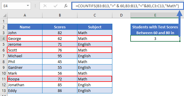

SUMPRODUCT Function

If you don’t have access to COUNTIFS, you can accomplish the same task with the SUMPRODUCT Function. The SUMPRODUCT Function opens up a world of possibilities with complex formulas (see SUMPRODUCT Tutorial). So, even if you have access to the COUNTIFS Function, you may want to start familiarizing yourself with this powerful function. It’s syntax is:

=SUMPRODUCT(Range 1=Condition 1*Range 2=Condition 2)

Using the same example above, to count all students with test scores above 60 in subject “Math”, you can use this formula:

=SUMPRODUCT((B3:B13>60)*(C3:C13="Math"))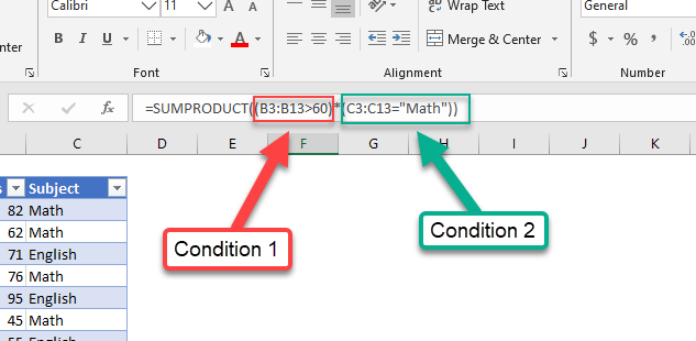

The first condition tests which values in that range are greater than 60, and the second condition tests which values in that range equal to “Math”. This gives us an array of Boolean values of 1 (TRUE) or 0 (FALSE):

=SUMPRODUCT(({82;62;71;76;95;45;55;56;72;85;86}>60)*({"Math";"Math";"English";"Math";"English";"Math";"English";"Math";"Math";"English";"English"}="Math"))

=SUMPRODUCT(({TRUE;TRUE;TRUE;TRUE;TRUE;FALSE;FALSE;FALSE;TRUE;TRUE;TRUE})*({TRUE;TRUE;FALSE;TRUE;FALSE;TRUE;FALSE;TRUE;TRUE;FALSE;FALSE}))

=SUMPRODUCT({1;1;0;1;0;0;0;0;1;0;0})

=4

The SUMPRODUCT Function then totals all items in the array, giving us the count of students who scored about 60 in math.

COUNTIFS and SUMPRODUCT for Multiple Criteria in Google Sheets

You can use the same formula structures as above in Google Sheets to count with multiple criteria.