
Counting is an integral part of data analysis, whether you are tallying the head count of a department in your organization or the number of units that were sold quarter-by-quarter. Excel provides multiple techniques that you can use to count cells, rows, or columns of data. To help you make the best choice, this article provides a comprehensive summary of methods, a downloadable workbook with interactive examples, and links to related topics for further understanding.
Download our examples
You can download an example workbook that gives examples to supplement the information in this article. Most sections in this article will refer to the appropriate worksheet within the example workbook that provides examples and more information.
Download examples to count values in a spreadsheet
In this article
-
Simple counting
-
Use AutoSum
-
Add a Subtotal row
-
Count cells in a list or Excel table column by using the SUBTOTAL function
-
-
Counting based on one or more conditions
-
Video: Use the COUNT, COUNTIF, and COUNTA functions
-
Count cells in a range by using the COUNT function
-
Count cells in a range based on a single condition by using the COUNTIF function
-
Count cells in a column based on single or multiple conditions by using the DCOUNT function
-
Count cells in a range based on multiple conditions by using the COUNTIFS function
-
Count based on criteria by using the COUNT and IF functions together
-
Count how often multiple text or number values occur by using the SUM and IF functions together
-
Count cells in a column or row in a PivotTable
-
-
Counting when your data contains blank values
-
Count nonblank cells in a range by using the COUNTA function
-
Count nonblank cells in a list with specific conditions by using the DCOUNTA function
-
Count blank cells in a contiguous range by using the COUNTBLANK function
-
Count blank cells in a non-contiguous range by using a combination of SUM and IF functions
-
-
Counting unique occurrences of values
-
Count the number of unique values in a list column by using Advanced Filter
-
Count the number of unique values in a range that meet one or more conditions by using IF, SUM, FREQUENCY, MATCH, and LEN functions
-
-
Special cases (count all cells, count words)
-
Count the total number of cells in a range by using ROWS and COLUMNS functions
-
Count words in a range by using a combination of SUM, IF, LEN, TRIM, and SUBSTITUTE functions
-
-
Displaying calculations and counts on the status bar
Simple counting
You can count the number of values in a range or table by using a simple formula, clicking a button, or by using a worksheet function.
Excel can also display the count of the number of selected cells on the Excel status bar. See the video demo that follows for a quick look at using the status bar. Also, see the section Displaying calculations and counts on the status bar for more information. You can refer to the values shown on the status bar when you want a quick glance at your data and don’t have time to enter formulas.
Video: Count cells by using the Excel status bar
Watch the following video to learn how to view count on the status bar.

Use AutoSum
Use AutoSum by selecting a range of cells that contains at least one numeric value. Then on the Formulas tab, click AutoSum > Count Numbers.

Excel returns the count of the numeric values in the range in a cell adjacent to the range you selected. Generally, this result is displayed in a cell to the right for a horizontal range or in a cell below for a vertical range.
Top of Page
Add a Subtotal row
You can add a subtotal row to your Excel data. Click anywhere inside your data, and then click Data > Subtotal.
Note: The Subtotal option will only work on normal Excel data, and not Excel tables, PivotTables, or PivotCharts.

Also, refer to the following articles:
-
Outline (group) data in a worksheet
-
Insert subtotals in a list of data in a worksheet
Top of Page
Count cells in a list or Excel table column by using the SUBTOTAL function
Use the SUBTOTAL function to count the number of values in an Excel table or range of cells. If the table or range contains hidden cells, you can use SUBTOTAL to include or exclude those hidden cells, and this is the biggest difference between SUM and SUBTOTAL functions.
The SUBTOTAL syntax goes like this:
SUBTOTAL(function_num,ref1,[ref2],…)

To include hidden values in your range, you should set the function_num argument to 2.
To exclude hidden values in your range, set the function_num argument to 102.
Top of Page
Counting based on one or more conditions
You can count the number of cells in a range that meet conditions (also known as criteria) that you specify by using a number of worksheet functions.
Video: Use the COUNT, COUNTIF, and COUNTA functions
Watch the following video to see how to use the COUNT function and how to use the COUNTIF and COUNTA functions to count only the cells that meet conditions you specify.
Top of Page
Count cells in a range by using the COUNT function
Use the COUNT function in a formula to count the number of numeric values in a range.

In the above example, A2, A3, and A6 are the only cells that contains numeric values in the range, hence the output is 3.
Note: A7 is a time value, but it contains text (a.m.), hence COUNT does not consider it a numerical value. If you were to remove a.m. from the cell, COUNT will consider A7 as a numerical value, and change the output to 4.
Top of Page
Count cells in a range based on a single condition by using the COUNTIF function
Use the COUNTIF function function to count how many times a particular value appears in a range of cells.

Top of Page
Count cells in a column based on single or multiple conditions by using the DCOUNT function
DCOUNT function counts the cells that contain numbers in a field (column) of records in a list or database that match conditions that you specify.
In the following example, you want to find the count of the months including or later than March 2016 that had more than 400 units sold. The first table in the worksheet, from A1 to B7, contains the sales data.

DCOUNT uses conditions to determine where the values should be returned from. Conditions are typically entered in cells in the worksheet itself, and you then refer to these cells in the criteria argument. In this example, cells A10 and B10 contain two conditions—one that specifies that the return value must be greater than 400, and the other that specifies that the ending month should be equal to or greater than March 31st, 2016.
You should use the following syntax:
=DCOUNT(A1:B7,»Month ending»,A9:B10)
DCOUNT checks the data in the range A1 through B7, applies the conditions specified in A10 and B10, and returns 2, the total number of rows that satisfy both conditions (rows 5 and 7).
Top of Page
Count cells in a range based on multiple conditions by using the COUNTIFS function
The COUNTIFS function is similar to the COUNTIF function with one important exception: COUNTIFS lets you apply criteria to cells across multiple ranges and counts the number of times all criteria are met. You can use up to 127 range/criteria pairs with COUNTIFS.
The syntax for COUNTIFS is:
COUNTIFS(criteria_range1, criteria1, [criteria_range2, criteria2],…)
See the following example:

Top of Page
Count based on criteria by using the COUNT and IF functions together
Let’s say you need to determine how many salespeople sold a particular item in a certain region or you want to know how many sales over a certain value were made by a particular salesperson. You can use the IF and COUNT functions together; that is, you first use the IF function to test a condition and then, only if the result of the IF function is True, you use the COUNT function to count cells.
Notes:
-
The formulas in this example must be entered as array formulas. If you have opened this workbook in Excel for Windows or Excel 2016 for Mac and want to change the formula or create a similar formula, press F2, and then press Ctrl+Shift+Enter to make the formula return the results you expect. In earlier versions of Excel for Mac, use
 +Shift+Enter.
 -
For the example formulas to work, the second argument for the IF function must be a number.

Top of Page
Count how often multiple text or number values occur by using the SUM and IF functions together
In the examples that follow, we use the IF and SUM functions together. The IF function first tests the values in some cells and then, if the result of the test is True, SUM totals those values that pass the test.
Example 1

The above function says if C2:C7 contains the values Buchanan and Dodsworth, then the SUM function should display the sum of records where the condition is met. The formula finds three records for Buchanan and one for Dodsworth in the given range, and displays 4.
Example 2

The above function says if D2:D7 contains values lesser than $9000 or greater than $19,000, then SUM should display the sum of all those records where the condition is met. The formula finds two records D3 and D5 with values lesser than $9000, and then D4 and D6 with values greater than $19,000, and displays 4.
Example 3

The above function says if D2:D7 has invoices for Buchanan for less than $9000, then SUM should display the sum of records where the condition is met. The formula finds that C6 meets the condition, and displays 1.
Important: The formulas in this example must be entered as array formulas. That means you press F2 and then press Ctrl+Shift+Enter. In earlier versions of Excel for Mac use  +Shift+Enter.
See the following Knowledge Base articles for additional tips:
-
XL: Using SUM(IF()) As an Array Function Instead of COUNTIF() with AND
-
XL: How to Count the Occurrences of a Number or Text in a Range
Top of Page
Count cells in a column or row in a PivotTable
A PivotTable summarizes your data and helps you analyze and drill down into your data by letting you choose the categories on which you want to view your data.
You can quickly create a PivotTable by selecting a cell in a range of data or Excel table and then, on the Insert tab, in the Tables group, clicking PivotTable.

Let’s look at a sample scenario of a Sales spreadsheet, where you can count how many sales values are there for Golf and Tennis for specific quarters.
Note: For an interactive experience, you can run these steps on the sample data provided in the PivotTable sheet in the downloadable workbook.
-
Enter the following data in an Excel spreadsheet.
-
Select A2:C8
-
Click Insert > PivotTable.
-
In the Create PivotTable dialog box, click Select a table or range, then click New Worksheet, and then click OK.
An empty PivotTable is created in a new sheet.
-
In the PivotTable Fields pane, do the following:
-
Drag Sport to the Rows area.
-
Drag Quarter to the Columns area.
-
Drag Sales to the Values area.
-
Repeat step c.
The field name displays as SumofSales2 in both the PivotTable and the Values area.
At this point, the PivotTable Fields pane looks like this:
-
In the Values area, click the dropdown next to SumofSales2 and select Value Field Settings.
-
In the Value Field Settings dialog box, do the following:
-
In the Summarize value field by section, select Count.
-
In the Custom Name field, modify the name to Count.
-
Click OK.
-
The PivotTable displays the count of records for Golf and Tennis in Quarter 3 and Quarter 4, along with the sales figures.
-


Top of Page
Counting when your data contains blank values
You can count cells that either contain data or are blank by using worksheet functions.
Count nonblank cells in a range by using the COUNTA function
Use the COUNTA function function to count only cells in a range that contain values.
When you count cells, sometimes you want to ignore any blank cells because only cells with values are meaningful to you. For example, you want to count the total number of salespeople who made a sale (column D).

COUNTA ignores the blank values in D3, D4, D8, and D11, and counts only the cells containing values in column D. The function finds six cells in column D containing values and displays 6 as the output.
Top of Page
Count nonblank cells in a list with specific conditions by using the DCOUNTA function
Use the DCOUNTA function to count nonblank cells in a column of records in a list or database that match conditions that you specify.
The following example uses the DCOUNTA function to count the number of records in the database that is contained in the range A1:B7 that meet the conditions specified in the criteria range A9:B10. Those conditions are that the Product ID value must be greater than or equal to 2000 and the Ratings value must be greater than or equal to 50.

DCOUNTA finds two rows that meet the conditions- rows 2 and 4, and displays the value 2 as the output.
Top of Page
Count blank cells in a contiguous range by using the COUNTBLANK function
Use the COUNTBLANK function function to return the number of blank cells in a contiguous range (cells are contiguous if they are all connected in an unbroken sequence). If a cell contains a formula that returns empty text («»), that cell is counted.
When you count cells, there may be times when you want to include blank cells because they are meaningful to you. In the following example of a grocery sales spreadsheet. suppose you want to find out how many cells don’t have the sales figures mentioned.

Note: The COUNTBLANK worksheet function provides the most convenient method for determining the number of blank cells in a range, but it doesn’t work very well when the cells of interest are in a closed workbook or when they do not form a contiguous range. The Knowledge Base article XL: When to Use SUM(IF()) instead of CountBlank() shows you how to use a SUM(IF()) array formula in those cases.
Top of Page
Count blank cells in a non-contiguous range by using a combination of SUM and IF functions
Use a combination of the SUM function and the IF function. In general, you do this by using the IF function in an array formula to determine whether each referenced cell contains a value, and then summing the number of FALSE values returned by the formula.
See a few examples of SUM and IF function combinations in an earlier section Count how often multiple text or number values occur by using the SUM and IF functions together in this topic.
Top of Page
Counting unique occurrences of values
You can count unique values in a range by using a PivotTable, COUNTIF function, SUM and IF functions together, or the Advanced Filter dialog box.
Count the number of unique values in a list column by using Advanced Filter
Use the Advanced Filter dialog box to find the unique values in a column of data. You can either filter the values in place or you can extract and paste them to a new location. Then you can use the ROWS function to count the number of items in the new range.
To use Advanced Filter, click the Data tab, and in the Sort & Filter group, click Advanced.
The following figure shows how you use the Advanced Filter to copy only the unique records to a new location on the worksheet.

In the following figure, column E contains the values that were copied from the range in column D.

Notes:
-
If you filter your data in place, values are not deleted from your worksheet — one or more rows might be hidden. Click Clear in the Sort & Filter group on the Data tab to display those values again.
-
If you only want to see the number of unique values at a quick glance, select the data after you have used the Advanced Filter (either the filtered or the copied data) and then look at the status bar. The Count value on the status bar should equal the number of unique values.
For more information, see Filter by using advanced criteria
Top of Page
Count the number of unique values in a range that meet one or more conditions by using IF, SUM, FREQUENCY, MATCH, and LEN functions
Use various combinations of the IF, SUM, FREQUENCY, MATCH, and LEN functions.
For more information and examples, see the section «Count the number of unique values by using functions» in the article Count unique values among duplicates.
Top of Page
Special cases (count all cells, count words)
You can count the number of cells or the number of words in a range by using various combinations of worksheet functions.
Count the total number of cells in a range by using ROWS and COLUMNS functions
Suppose you want to determine the size of a large worksheet to decide whether to use manual or automatic calculation in your workbook. To count all the cells in a range, use a formula that multiplies the return values using the ROWS and COLUMNS functions. See the following image for an example:

Top of Page
Count words in a range by using a combination of SUM, IF, LEN, TRIM, and SUBSTITUTE functions
You can use a combination of the SUM, IF, LEN, TRIM, and SUBSTITUTE functions in an array formula. The following example shows the result of using a nested formula to find the number of words in a range of 7 cells (3 of which are empty). Some of the cells contain leading or trailing spaces — the TRIM and SUBSTITUTE functions remove these extra spaces before any counting occurs. See the following example:

Now, for the above formula to work correctly, you have to make this an array formula, otherwise the formula returns the #VALUE! error. To do that, click on the cell that has the formula, and then in the Formula bar, press Ctrl + Shift + Enter. Excel adds a curly bracket at the beginning and the end of the formula, thus making it an array formula.
For more information on array formulas, see Overview of formulas in Excel and Create an array formula.
Top of Page
Displaying calculations and counts on the status bar
When one or more cells are selected, information about the data in those cells is displayed on the Excel status bar. For example, if four cells on your worksheet are selected, and they contain the values 2, 3, a text string (such as «cloud»), and 4, all of the following values can be displayed on the status bar at the same time: Average, Count, Numerical Count, Min, Max, and Sum. Right-click the status bar to show or hide any or all of these values. These values are shown in the illustration that follows.

Top of Page
Need more help?
You can always ask an expert in the Excel Tech Community or get support in the Answers community.
Содержание
- Процедура подсчета значений в столбце
- Способ 1: индикатор в строке состояния
- Способ 2: оператор СЧЁТЗ
- Способ 3: оператор СЧЁТ
- Способ 4: оператор СЧЁТЕСЛИ
- Вопросы и ответы

В некоторых случаях перед пользователем ставится задача не подсчета суммы значений в столбце, а подсчета их количества. То есть, попросту говоря, нужно подсчитать, сколько ячеек в данном столбце заполнено определенными числовыми или текстовыми данными. В Экселе существует целый ряд инструментов, которые способны решить указанную проблему. Рассмотрим каждый из них в отдельности.
Читайте также: Как посчитать количество строк в Excel
Как посчитать количество заполненных ячеек в Экселе
Процедура подсчета значений в столбце
В зависимости от целей пользователя, в Экселе можно производить подсчет всех значений в столбце, только числовых данных и тех, которые соответствуют определенному заданному условию. Давайте рассмотрим, как решить поставленные задачи различными способами.
Способ 1: индикатор в строке состояния
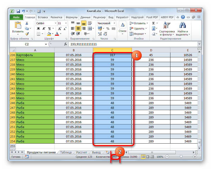
Данный способ самый простой и требующий минимального количества действий. Он позволяет подсчитать количество ячеек, содержащих числовые и текстовые данные. Сделать это можно просто взглянув на индикатор в строке состояния.
Для выполнения данной задачи достаточно зажать левую кнопку мыши и выделить весь столбец, в котором вы хотите произвести подсчет значений. Как только выделение будет произведено, в строке состояния, которая расположена внизу окна, около параметра «Количество» будет отображаться число значений, содержащихся в столбце. В подсчете будут участвовать ячейки, заполненные любыми данными (числовые, текстовые, дата и т.д.). Пустые элементы при подсчете будут игнорироваться.
В некоторых случаях индикатор количества значений может не высвечиваться в строке состояния. Это означает то, что он, скорее всего, отключен. Для его включения следует кликнуть правой кнопкой мыши по строке состояния. Появляется меню. В нем нужно установить галочку около пункта «Количество». После этого количество заполненных данными ячеек будет отображаться в строке состояния.

К недостаткам данного способа можно отнести то, что полученный результат нигде не фиксируется. То есть, как только вы снимете выделение, он исчезнет. Поэтому, при необходимости его зафиксировать, придется записывать полученный итог вручную. Кроме того, с помощью данного способа можно производить подсчет только всех заполненных значениями ячеек и нельзя задавать условия подсчета.
Способ 2: оператор СЧЁТЗ
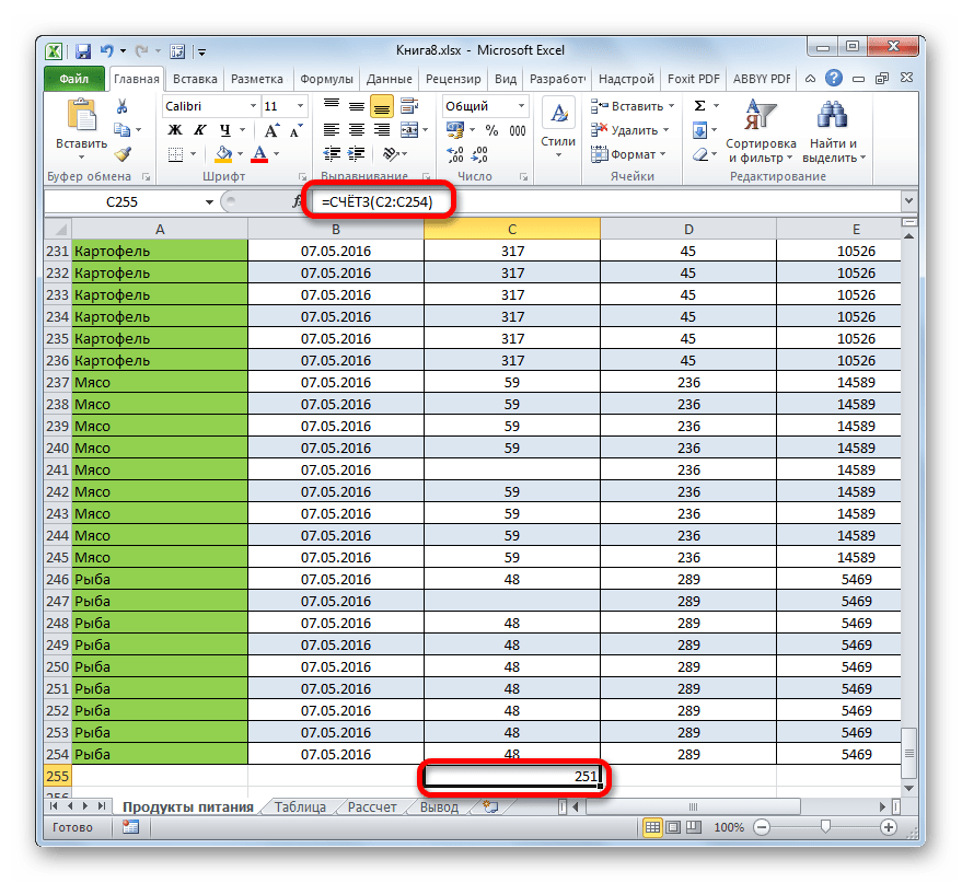
С помощью оператора СЧЁТЗ, как и в предыдущем случае, имеется возможность подсчета всех значений, расположенных в столбце. Но в отличие от варианта с индикатором в панели состояния, данный способ предоставляет возможность зафиксировать полученный результат в отдельном элементе листа.
Главной задачей функции СЧЁТЗ, которая относится к статистической категории операторов, как раз является подсчет количества непустых ячеек. Поэтому мы её с легкостью сможем приспособить для наших нужд, а именно для подсчета элементов столбца, заполненных данными. Синтаксис этой функции следующий:
=СЧЁТЗ(значение1;значение2;…)
Всего у оператора может насчитываться до 255 аргументов общей группы «Значение». В качестве аргументов как раз выступают ссылки на ячейки или диапазон, в котором нужно произвести подсчет значений.
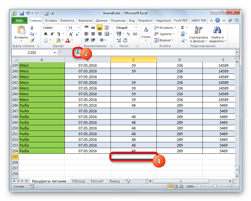
- Выделяем элемент листа, в который будет выводиться итоговый результат. Щелкаем по значку «Вставить функцию», который размещен слева от строки формул.
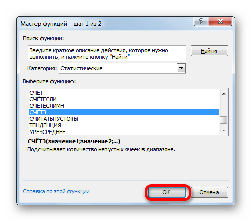
- Тем самым мы вызвали Мастер функций. Переходим в категорию «Статистические» и выделяем наименование «СЧЁТЗ». После этого производим щелчок по кнопке «OK» внизу данного окошка.
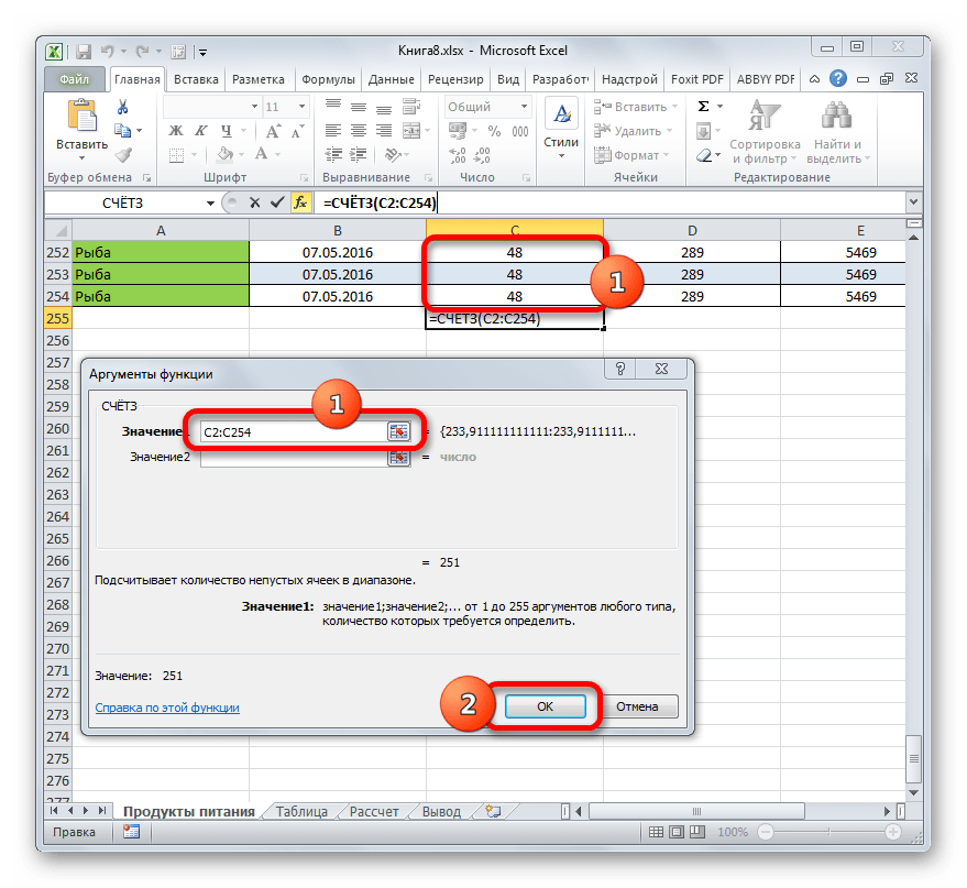
- Мы переходим к окну аргументов функции СЧЁТЗ. В нём располагаются поля ввода аргументов. Как и количество аргументов, они могут достигать численности 255 единиц. Но для решения поставленной перед нами задачи хватит и одного поля «Значение1». Устанавливаем в него курсор и после этого с зажатой левой кнопкой мыши выделяем на листе тот столбец, значения в котором нужно подсчитать. После того, как координаты столбца отобразились в поле, жмем на кнопку «OK» в нижней части окна аргументов.
- Программа производит подсчет и выводит в ячейку, которую мы выделяли на первом шаге данной инструкции, количество всех значений (как числовых, так и текстовых), содержащихся в целевом столбце.

Как видим, в отличие от предыдущего способа, данный вариант предлагает выводить результат в конкретный элемент листа с возможным его сохранением там. Но, к сожалению, функция СЧЁТЗ все-таки не позволяет задавать условия отбора значений.
Урок: Мастер функций в Excel
Способ 3: оператор СЧЁТ
С помощью оператора СЧЁТ можно произвести подсчет только числовых значений в выбранной колонке. Он игнорирует текстовые значения и не включает их в общий итог. Данная функция также относится к категории статистических операторов, как и предыдущая. Её задачей является подсчет ячеек в выделенном диапазоне, а в нашем случае в столбце, который содержит числовые значения. Синтаксис этой функции практически идентичен предыдущему оператору:
=СЧЁТ(значение1;значение2;…)
Как видим, аргументы у СЧЁТ и СЧЁТЗ абсолютно одинаковые и представляют собой ссылки на ячейки или диапазоны. Различие в синтаксисе заключается лишь в наименовании самого оператора.
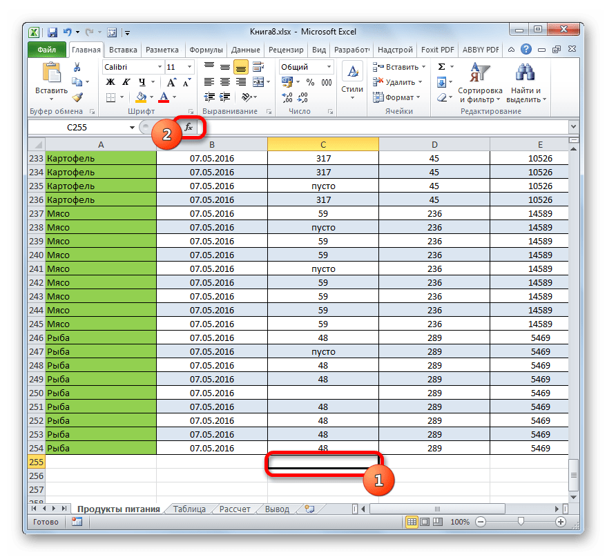
- Выделяем элемент на листе, куда будет выводиться результат. Нажимаем уже знакомую нам иконку «Вставить функцию».
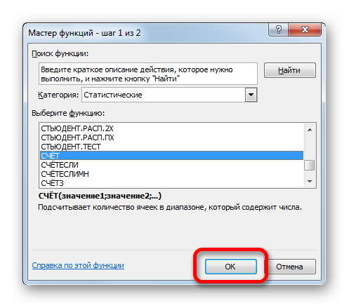
- После запуска Мастера функций опять перемещаемся в категорию «Статистические». Затем выделяем наименование «СЧЁТ» и щелкаем по кнопке «OK».
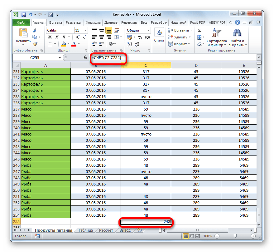
- После того, как было запущено окно аргументов оператора СЧЁТ, следует в его поле внести запись. В этом окне, как и в окне предыдущей функции, тоже может быть представлено до 255 полей, но, как и в прошлый раз, нам понадобится всего одно из них под названием «Значение1». Вводим в это поле координаты столбца, над которым нам нужно выполнить операцию. Делаем это все тем же образом, каким выполняли данную процедуру для функции СЧЁТЗ: устанавливаем курсор в поле и выделяем колонку таблицы. После того, как адрес столбца был занесен в поле, жмем на кнопку «OK».
- Результат тут же будет выведен в ячейку, которую мы определили для содержания функции. Как видим, программа подсчитала только ячейки, которые содержат числовые значения. Пустые ячейки и элементы, содержащие текстовые данные, в подсчете не участвовали.

Урок: Функция СЧЁТ в Excel
Способ 4: оператор СЧЁТЕСЛИ
В отличие от предыдущих способов, использование оператора СЧЁТЕСЛИ позволяет задавать условия, отвечающие значения, которые будут принимать участие в подсчете. Все остальные ячейки будут игнорироваться.
Оператор СЧЁТЕСЛИ тоже причислен к статистической группе функций Excel. Его единственной задачей является подсчет непустых элементов в диапазоне, а в нашем случае в столбце, которые отвечают заданному условию. Синтаксис у данного оператора заметно отличается от предыдущих двух функций:
=СЧЁТЕСЛИ(диапазон;критерий)
Аргумент «Диапазон» представляется в виде ссылки на конкретный массив ячеек, а в нашем случае на колонку.
Аргумент «Критерий» содержит заданное условие. Это может быть как точное числовое или текстовое значение, так и значение, заданное знаками «больше» (>), «меньше» (<), «не равно» (<>) и т.д.
Посчитаем, сколько ячеек с наименованием «Мясо» располагаются в первой колонке таблицы.
- Выделяем элемент на листе, куда будет производиться вывод готовых данных. Щелкаем по значку «Вставить функцию».
- В Мастере функций совершаем переход в категорию «Статистические», выделяем название СЧЁТЕСЛИ и щелкаем по кнопке «OK».
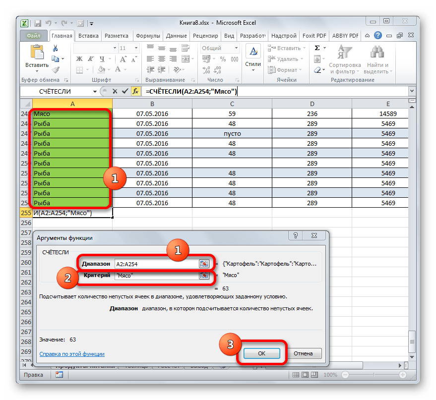
- Производится активация окошка аргументов функции СЧЁТЕСЛИ. Как видим, окно имеет два поля, которые соответствуют аргументам функции.
В поле «Диапазон» тем же способом, который мы уже не раз описывали выше, вводим координаты первого столбца таблицы.
В поле «Критерий» нам нужно задать условие подсчета. Вписываем туда слово «Мясо».
После того, как вышеуказанные настройки выполнены, жмем на кнопку «OK».
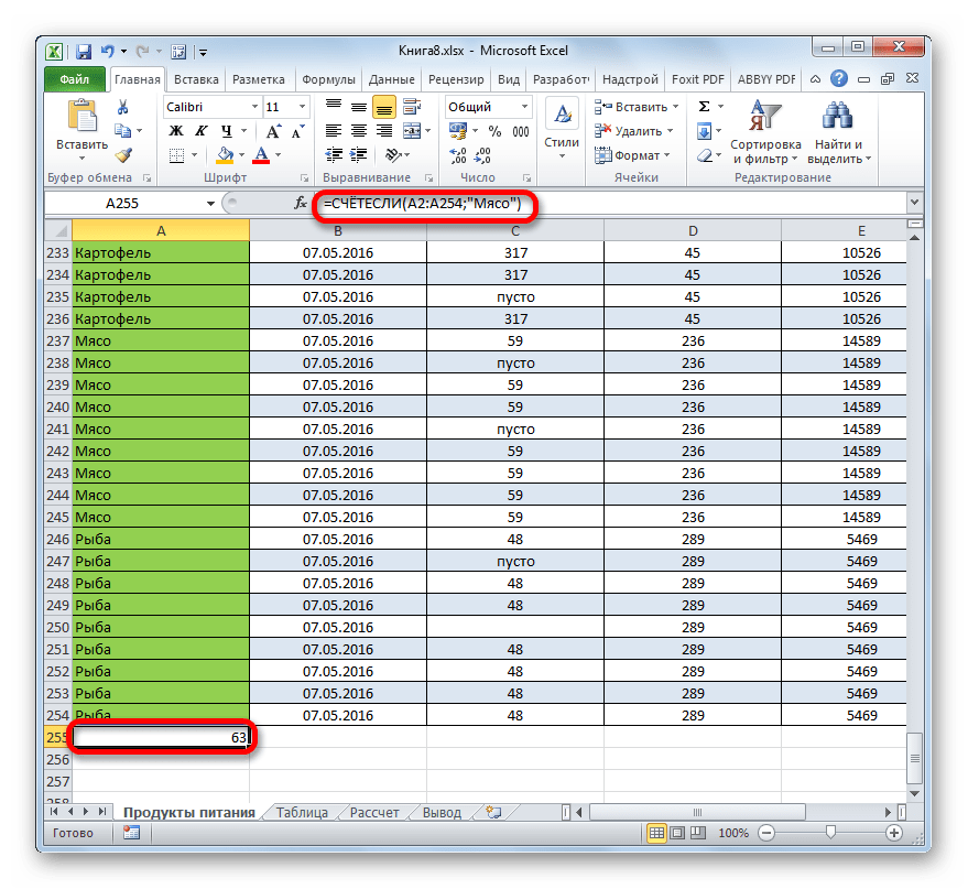
- Оператор производит вычисления и выдает результат на экран. Как видим, в выделенной колонке в 63 ячейках содержится слово «Мясо».

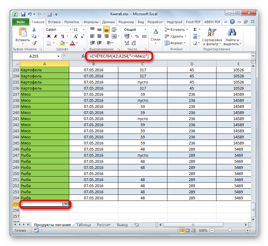
Давайте немного изменим задачу. Теперь посчитаем количество ячеек в этой же колонке, которые не содержат слово «Мясо».
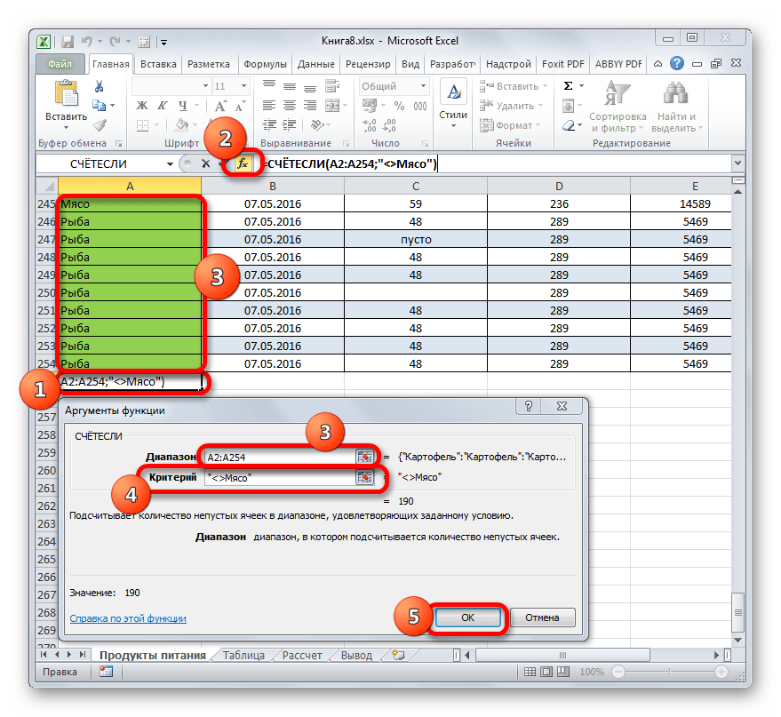
- Выделяем ячейку, куда будем выводить результат, и уже описанным ранее способом вызываем окно аргументов оператора СЧЁТЕСЛИ.
В поле «Диапазон» вводим координаты все того же первого столбца таблицы, который обрабатывали ранее.
В поле «Критерий» вводим следующее выражение:
<>МясоТо есть, данный критерий задает условие, что мы подсчитываем все заполненные данными элементы, которые не содержат слово «Мясо». Знак «<>» означает в Экселе «не равно».
После введения этих настроек в окне аргументов жмем на кнопку «OK».
- В предварительно заданной ячейке сразу же отображается результат. Он сообщает о том, что в выделенном столбце находятся 190 элементов с данными, которые не содержат слово «Мясо».
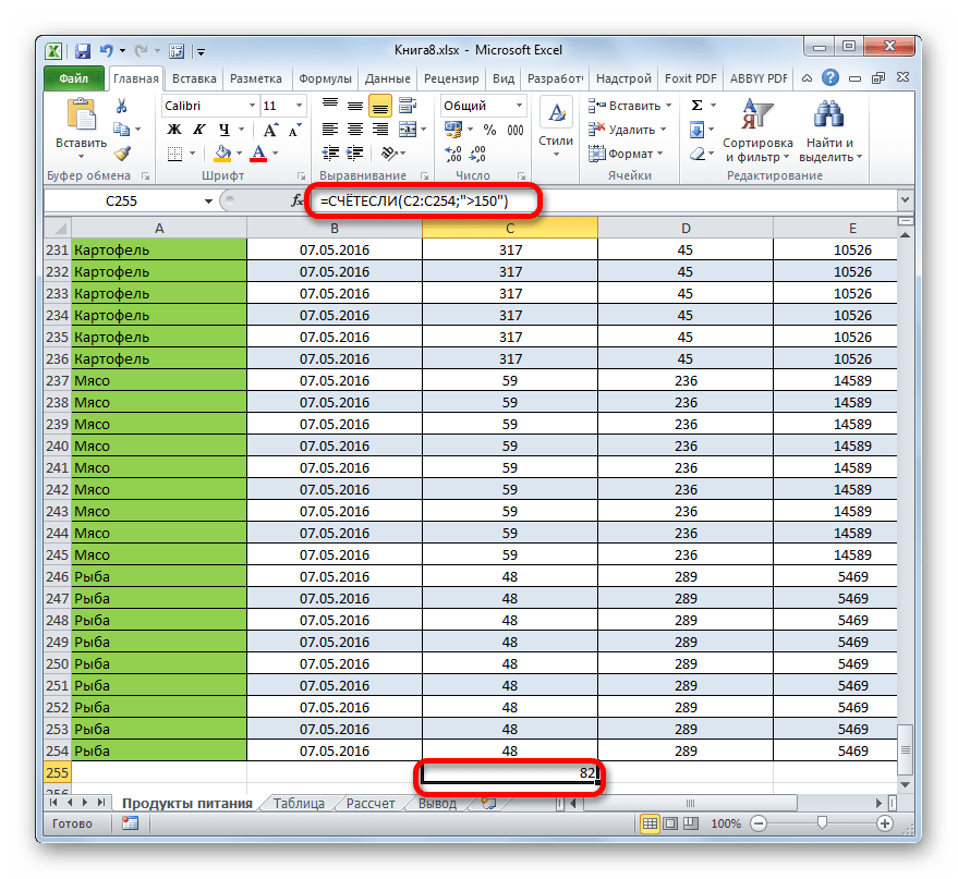
Теперь давайте произведем в третьей колонке данной таблицы подсчет всех значений, которые больше числа 150.
- Выделяем ячейку для вывода результата и производим переход в окно аргументов функции СЧЁТЕСЛИ.
В поле «Диапазон» вводим координаты третьего столбца нашей таблицы.
В поле «Критерий» записываем следующее условие:
>150Это означает, что программа будет подсчитывать только те элементы столбца, которые содержат числа, превышающие 150.
Далее, как всегда, жмем на кнопку «OK».
- После проведения подсчета Excel выводит в заранее обозначенную ячейку результат. Как видим, выбранный столбец содержит 82 значения, которые превышают число 150.

Таким образом, мы видим, что в Excel существует целый ряд способов подсчитать количество значений в столбце. Выбор определенного варианта зависит от конкретных целей пользователя. Так, индикатор на строке состояния позволяет только посмотреть количество всех значений в столбце без фиксации результата; функция СЧЁТЗ предоставляет возможность их число зафиксировать в отдельной ячейке; оператор СЧЁТ производит подсчет только элементов, содержащих числовые данные; а с помощью функции СЧЁТЕСЛИ можно задать более сложные условия подсчета элементов.
To count the number of different values in A2:A100 (not counting blanks):
=SUMPRODUCT((A2:A100<>"")/COUNTIF(A2:A100,A2:A100&""))
Copied from an answer by @Ulli Schmid to What is this COUNTIF() formula doing?:
=SUMPRODUCT((A1:A100<>"")/COUNTIF(A1:A100,A1:A100&""))
Counts unique cells within A1:A100, excluding blank cells and ones with an empty string («»).
How does it do that? Example:
A1:A100 = [1, 1, 2, "apple", "peach", "apple", "", "", -, -, -, ...]
then:
A1:A100&"" = ["1", "1", "2", "apple", "peach", "apple", "", "", "", "", "", ...]
so this &»» is needed to turn blank cells (-) into empty strings («»). If you were to count directly using blank cells, COUNTIF() returns 0. Using the trick, both «» and — are counted as the same:
COUNTIF(A1:A100,A1:A100) = [2, 2, 1, 2, 1, 2, 94, 94, 0, 0, 0, ...]
but:
COUNTIF(A1:A100,A1:A100&"") = [2, 2, 1, 2, 1, 2, 94, 94, 94, 94, 94, ...]
If we now want to get the count of all unique cells, excluding blanks and «», we can divide
(A1:A100<>""), which is [1, 1, 1, 1, 1, 1, 0, 0, 0, 0, 0, ...]
by our intermediate result, COUNTIF(A1:A100,A1:A100&»»), and sum up over the values.
SUMPRODUCT((A1:A100<>"")/COUNTIF(A1:A100,A1:A100&""))
= (1/2 + 1/2 + 1/1 + 1/2 + 1/1 + 1/2 + 0/94 + 0/94 + 0/94 + 0/94 + 0/94 + ...)
= 4
Had we used COUNTIF(A1:A100,A1:A100) instead of COUNTIF(A1:A100,A1:A100&""), then some of those 0/94 would have been 0/0. As division by zero is not allowed, we would have thrown an error.
How to Use the COUNT function in Excel (and COUNTA)
Apart from storing and manipulating numbers, sometimes, you may want to use Excel to simply count numbers.
For example, the number of students in a class, the number of items on a list, etc.
To do so, Excel offers two functions, the COUNT and the COUNTA function. Both the said functions are super easy to operate and can prove very handy. 😀
Read through this tutorial till the end to master both these functions. Also, download our free sample workbook right here to practice alongside you read.
How to use the COUNT function to count cells in Excel
The COUNT function of Excel is going to be one of the simplest functions you’d ever come across.
Take the data in the image below.

1. To count these cells, write the COUNT function as follows.
=COUNT (A1:A6)

2. Here is the count produced by Excel.

Must note how the COUNT function has ignored the blank cell in between.
Pro Tip!
Did you notice how the COUNT function gives results that are not obvious to the eyes? We can see there are five values in the above formula.
The COUNT formula, however, only returns 4 as the count.
This is because the COUNT function only counts certain values that are either:
- Numeric values
- Date and Time values
- Boolean values (TRUE/FALSE)
- Numeric values enclosed in quotation marks (like “10”)
Umbrella is a text value, hence ignored by the COUNT function.
3. If you do not have a cell range to specify, you may also specify values inside the formula separated by a comma.
=COUNT (1, 2, 12/12/22, hello)

Must know that Excel 2007 (and newer versions) can only accept up to 255 values (arguments).
Until Excel 2007, this number was only 30. 🤨
Counting cells in non-adjacent ranges
Can the COUNT function tackle non-adjacent ranges like in the image below?

1. Write the following formula.
=COUNT (A1:A5, B1:B6, C1:C10)

We have specified each non-adjacent range as a separate argument.
2. The COUNT function counts all the non-blank cells.

COUNT vs COUNTA: Count numbers or non-empty cells
What differentiates the COUNT and COUNTA functions? A few things.
1. The COUNT function only counts cells containing specified values. These values include numbers, dates, time, and logical values (TRUE / FALSE). It also counts in numerical values enclosed in Quotation marks (“”).
Any value other than these would not be counted in by the COUNT function. It also ignores any text string.

2. The COUNT function ignores any blank cell in the specified range.

3. The COUNTA function only counts all non-blank cells.

A blank cell means a cell is all blank (no value). If a cell is only apparently blank, the COUNTA function would treat it as a non-blank cell and count it in.
An apparently blank cell may be the one with space even. Or some function the result whereof is a blank cell.
How to use the COUNTA function to count non-empty cells
It’s time we see how the COUNTA function works.
The COUNTA function counts all non-blank cells (containing any values).
Let’s apply the COUNTA function to the data in the image below.

1. Write the COUNTA function as below.
= COUNTA (A1:A10)
2. COUNTA gives the results as follows.

The results show 8 cells. However, we only see 7 cells that contain values.
That’s what you see. One cell in between doesn’t have a value but a space character.

Even if a cell has a space character, the COUNTA function doesn’t treat it as a blank cell. It is included in the count of cells. 😏
The COUNTA function counts all values including text values and ERROR values. Error values include errors posed by Excel like the #NAME! error etc.
Count cells using the status bar
If you’re running out of time and want a quick count of cells containing data – this section is for you.
You can count non-blank cells in Excel without operating a function.
1. Select the cells containing data.
Navigate to the right bottom of your spreadsheet to see the count of cells.

2. Or you can select multiple column headers (or row headers). In this case, Excel will count the number of non-blank cells in each column (or row).

That’s it – Now what?
This guide teaches you the basics of the COUNT and COUNTA functions. It differentiates between them both and explains when should you use each of them.
Both the COUNT and COUNTA functions would help you in many situations. But these are only two very basic functions of Excel.
There’s much more to learn from this giant spreadsheet software. Some functions of Excel that you MUST learn are the VLOOKUP, SUMIF, and IF functions.
Register for my 30-minute free email course that is designed to offer you insights into these functions (and more).
Other resources
There are many advanced versions of the COUNT and COUNTA functions of Excel. For example the COUNTIF function and the COUNTIFS function.
The COUNTIF function counts cells that meet a single criterion. Whereas, the COUNTIFS function counts cells that meet multiple criteria. Check them out here!
Additionally, you may want to learn how to use operators in the COUNTIF Function.
Kasper Langmann2022-11-03T07:04:06+00:00
Page load link
Microsoft Word allows you count text, but what about Excel? If you need a count of your text in Excel, you can get this by using the COUNTIF function and then a combination of other functions depending on your desired result.
How to count text in Excel
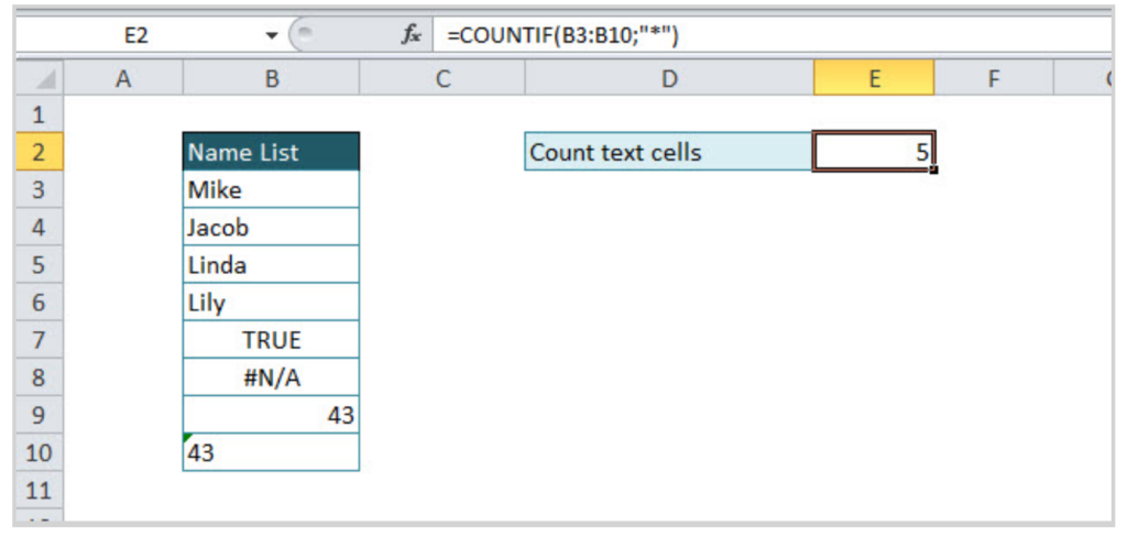
If you want to learn how to count text in Excel, you need to use function COUNTIF with the criteria defined using wildcard *, with the formula: =COUNTIF(range;"*"). Range is defined cell range where you want to count the text in Excel and wildcard * is criteria for all text occurrences in the defined range.
Some interesting and very useful examples will be covered in this tutorial with the main focus on the COUNTIF function and different usages of this function in text counting. Limitations of COUNTIF function have been covered in this tutorial with an additional explanation of other functions such as SUMPRODUCT/ISNUMBER/FIND functions combination. After this tutorial, you will be able to count text cells in excel, count specific text cells, case sensitive text cells and text cells with multiple criteria defined – which is a very good base for further creative Excel problem-solving.
Count Text Cells in Excel
Text Cells can be easily found in Excel using COUNTIF or COUNTIFS functions. The COUNTIF function searches text cells based on specific criteria and in the defined range. As in the example below, the defined range is table Name list, and text criteria is defined using wildcard “*”. The formula result is 5, all text cells have been counted. Note that number formatted as text in cell B10 is also counted, but Booleans (TRUE /FALSE) and error (#N/A) are not recognized as text.
The formula for counting text cells:
=COUNTIF(range;"*")
For counting non-text cells, the formula should be a little bit changed in criteria part:
=COUNTIF(range;"<>*")
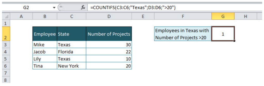
If there are several criteria for counting cells, then COUNTIFS function should be used. For example, if we want to count the number of employees from Texas with project number greater than 20, then the function will look like:
=COUNTIFS(C3:C6;"Texas";D3:D6;">20").
In criteria range in column State, a specific text criteria is defined under quotations “Texas”. The second criteria is numeric, criteria range is column Number of projects, and criteria is numeric value greater than 20, also under quotations “>20”. If we were looking for exact value, the formula would look like:
=COUNTIFS(C3:C6;"Texas";D3:D6;20)
Count Specific Text in Cells
For counting specific text under cells range, COUNTIF function is suitable with the formula:
=COUNTIF(range;"*text*")
=COUNTIF(B3:B9;"*Mike*")
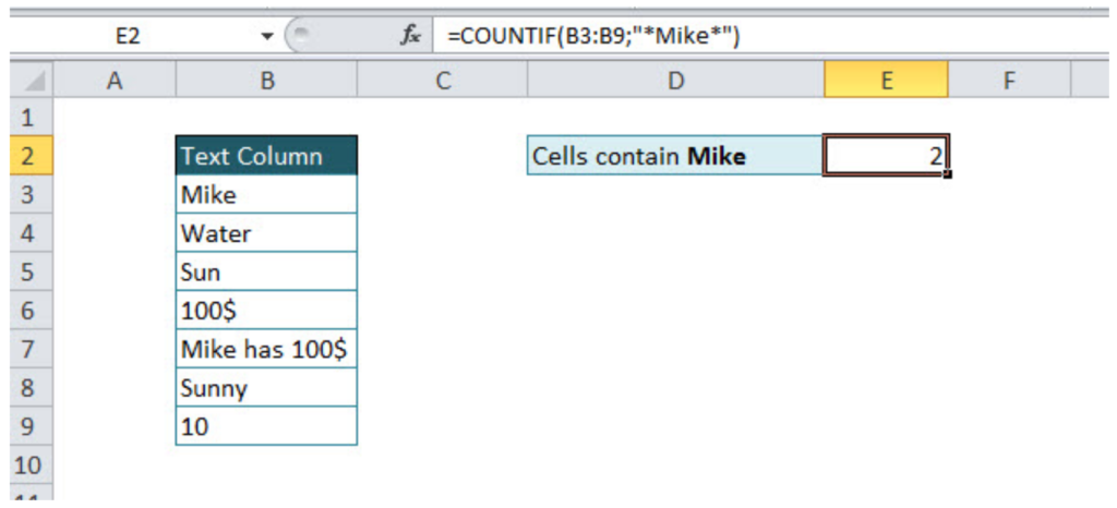
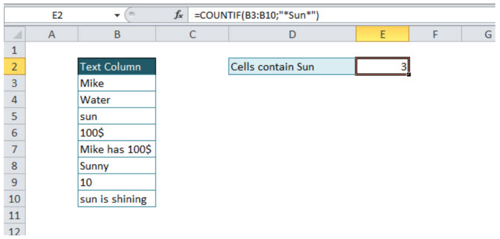
The first part of the formula is range and second is text criteria, in our example “*Mike*”. If wildcard * has not been used before and after criteria text, formula result would have been 1 (Formula would find cells only with word Mike). Wildcard * before and after criteria text, means that all cells that contain criteria characters will be taken into account. As in another example below with text criteria Sun, three cells were found (sun, Sunny, sun is shining)
=COUNTIF(B3:B10;"*Sun*")
Note: The COUNTIF function is not case sensitive, an alternative function for case sensitive text searches is SUMPRODUCT/FIND function combination.
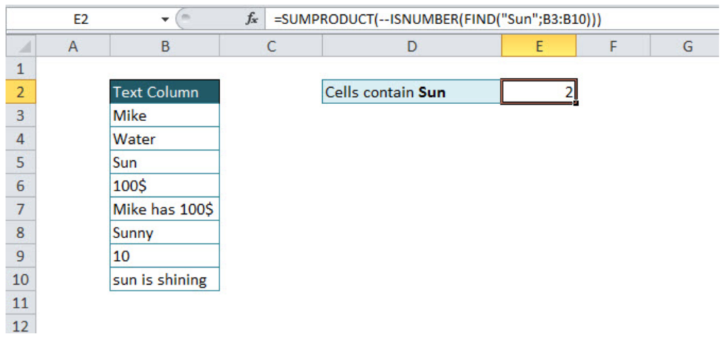
Count Case Sensitive Specific Text
For a case-sensitive text count, a combination of three formulas should be used: SUMPRODUCT, ISNUMBER and FIND. Let’s look in the example below. If we want to count cells that contain text Sun, case sensitive, COUNTIF function would not be the appropriate solution, instead of this function combination of three functions mentioned above has to be used.
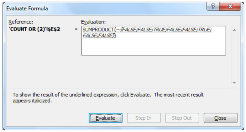
=SUMPRODUCT(--ISNUMBER(FIND("Sun";B3:B10)))
We should go through a separate function explanation in order to understand functions combination. FIND function, searches specific text in the defined cell, and returns the number of the starting position of the text used as criteria. This explanation is relevant, if the searching range is just one cell. If we want to use FIND function in a range of the cells, then the combination with SUMPRODUCT function is necessary.
Without ISNUMBER, function combination of FIND and SUMPRODUCT functions would return an error. ISNUMBER function is necessary because whenever FIND function does not match defined criteria, the output will be an error, as in print screen below of the evaluated formula.
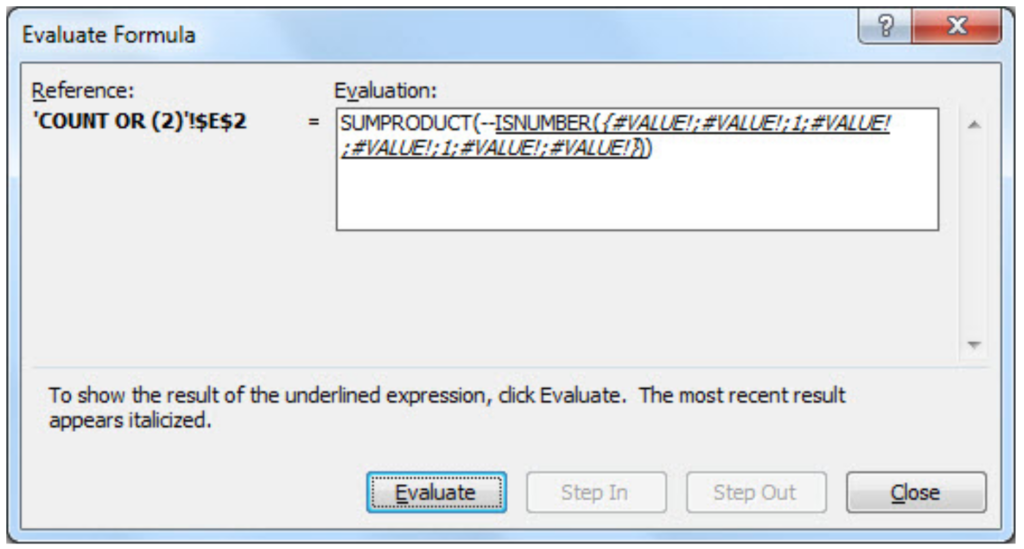
In order to change error values with Boolean TRUE/FALSE statement, ISNUMERIC formula should be used (defining numeric values as TRUE, and non-numeric as FALSE, as in print screen below).
You might be wondering what character — in SUMPRODUCT function stands for. It converts Boolean values TRUE/FALSE in numeric values 1/0, enabling SUMPRODUCT function to deal with numeric operations (without character — in SUMPRODUCT function, the final result would be 0).
Remember, if you want to count specific text cells that are not case sensitive, COUNTIF function is suitable. For all case sensitive searches combination of SUMPRODUCT/ISNUMBER/FIND functions is appropriate.
Count Text Cells with Multiple Criteria
If you want to count cells with Multiple criteria, with all criteria acceptable, there is an interesting way of solving that problem, a combination of SUMPRODUCT/ISNUMBER/FIND functions. Please take a look in the example below. We should count all cells that contain either Mike or $. Tricky part could be the cells that contain both Mike and $.
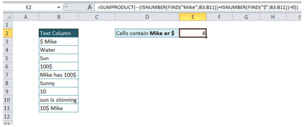
=SUMPRODUCT(--(ISNUMBER(FIND("Mike";B3:B11))+ISNUMBER(FIND("$";B3:B11))>0))
Formula just looks complex, in order to be easier for understanding, I will divide it into several steps. Also, knowledge from the previous tutorial point will be necessary for further work, since the combination of FIND, ISNUMBER, and SUMPRODUCT functions have been explained.
In the first part of the function, we loop through the table and find cells that contain Mike:
=ISNUMBER(FIND("Mike";B3:B11))
The output of this part of the function will be an array with values {1;0;0;0;1;0;0;0;1}, number 1, where criteria have been met, and 0, where has not.
In the second part of the function, looping criteria is $, counting cells containing this value:
=ISNUMBER(FIND("$";B3:B11))
The output of this part of the function will be an array with values {1;0;0;1;1;0;0;0;1}, number 1, where criteria have been met, and 0, where has not.
Next step is to sum these two arrays, since cell should be counted if any of conditions is fulfilled:
=ISNUMBER(FIND("Mike";B3:B11))+ISNUMBER(FIND("$";B3:B11))
The output of this step is {2;0;0;1;2;0;0;0;2}, the number greater than 0 means that one of the condition has been met (2 – both conditions, 1 – one condition)
Without function part >0, the final function would double count cells that met both conditions and the final result would be 7 (sum of all array numbers). In order to avoid it, in the formula should be added >0:
=ISNUMBER(FIND("Mike";B3:B11))+ISNUMBER(FIND("$";B3:B11))>0
The output of this step is array {1;0;0;1;1;0;0;0;1}, the previous array has been checked and only values greater than 0 are TRUE (in an array have value 1), and others are FALSE (in an array have value 0).
Final output of the formula is the sum of the final array values, 4.
Looks very confusing, but after several usages, you will become familiar with this functions.
At the end, we will cover one more multiple criteria text count function, already mentioned in the tutorial, COUNTIFS function. In order to distinguish the usage of functions mentioned above and COUNTIFS function, two words are enough OR/AND. If you want to count text cells with multiple criteria but all conditions have to be met at the same time, then COUNTIFS function is appropriate. If at least one condition should be met, then the combination of function explained above is suitable.
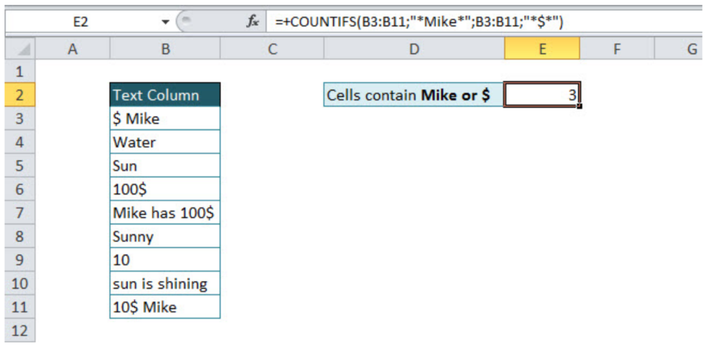
Look at the example below, the number of cells that contain both Mike and $ is easily calculated with COUNTIFS function:
=COUNTIFS(range1;"*text1*";range2;"*text2*")
=COUNTIFS(B3:B11;"*Mike*";B3:B11;"*$*")
In the defined range, function counts only cells where both conditions have been met. The final result is 3.
Still need some help with Excel formatting or have other questions about Excel? Connect with a live Excel expert here for some 1 on 1 help. Your first session is always free.