
Watch Video – How to Count Cells that Contain Text Strings
Counting is one of the most common tasks people do in Excel. It’s one of the metric that is often used to summarize the data. For example, count sales done by Bob, or sales more than 500K or quantity of Product X sold.
Excel has a variety of count functions, and in most cases, these inbuilt Excel functions would suffice. Below are the count functions in Excel:
- COUNT – To count the number of cells that have numbers in it.
- COUNTA – To count the number of cells that are not empty.
- COUNTBLANK – To count blank cell.
- COUNTIF/COUNTIFS – To count cells when the specified criteria are met.
There may sometimes be situations where you need to create a combination of functions to get the counting done in Excel.
One such case is to count cells that contain text strings.
Count Cells that Contain Text in Excel
Text values can come in many forms. It could be:
- Text String
- Text Strings or Alphanumeric characters. Example – Trump Excel or Trump Excel 123.
- Empty String
- A cell that looks blank but contains =”” or ‘ (if you just type an apostrophe in a cell, it looks blank).
- Logical Values
- Example – TRUE and FALSE.
- Special characters
- Example – @, !, $ %.
Have a look at the data set shown below:
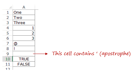
It has all the combinations of text, numbers, blank, special characters, and logical values.
To count cells that contain text values, we will use the wildcard characters:
- Asterisk (*): An asterisk represents any number of characters in excel. For example, ex* could mean excel, excels, example, expert, etc.
- Question Mark (?): A question mark represents one single character. For example, Tr?mp could mean Trump or Tramp.
- Tilde (~): To identify wildcard characters in a string.
See Also: Examples of using Wildcard Characters in Excel.
Now let’s create formulas to count different combinations.
Count Cells that Contain Text in Excel (including Blanks)
Here is the formula:
=COUNTIF(A1:A11,”*”)
This formula uses COUNTIF function with a wildcard character in the criteria. Since asterisk (*) represents any number of characters, it counts all the cells that have text characters in it.
It even counts cells that have an empty string in it (an empty string can be a result of formula returning =”” or a cell that contains an apostrophe). While a cell with empty string looks blank, it is counted by this formula.
Logical Values are not counted.

Count Cells that Contain Text in Excel (excluding Blanks)
Here is the formula:
=COUNTIF(A1:A11,”?*”)
In this formula, the criteria argument is made up of a combination of two wildcard characters (question mark and asterisk). This means that there should, at least, be one character in the cell.
This formula does not count cells that contain an empty string (an apostrophe or =””). Since an empty string has no character in it, it fails the criteria and is not counted.
Logical Values are also not counted.

Count Cells that Contain Text (excluding Blanks, including Logical Values)
Here is the formula:
=COUNTIF(A1:A11,”?*”) + SUMPRODUCT(–(ISLOGICAL(A1:A11))
The first part of the formula uses a combination of wildcard characters (* and ?). This returns the number of cells that have at least one text character in it (counts text and special characters, but does not count cells with empty strings).
The second part of the formula checks for logical values. Excel ISLOGICAL function returns TRUE if there is a logical value and FALSE if there isn’t. A double negative sign ensures that TRUEs are converted into 1 and FALSEs into 0. Excel SUMPRODUCT function then simply returns the number of cells that have a logical value in it.

These above examples demonstrate how to use a combination of formulas and wildcard characters to count cells. In a similar fashion, you can also construct formulas to find the SUM or AVERAGE of a range of cells based on the data type in it.
You May Also Like the Following Excel Tutorials:
- Count the Number of Words in a Text String.
- Using Multiple Criteria in Excel COUNTIF and COUNTIFS Function.
- How to Count Colored Cells in Excel.
- Count Characters in a Cell (or Range of Cells) Using Formulas in Excel
If you want to learn how to count text in Excel, you need to use function COUNTIF with the criteria defined using wildcard *, with the formula: =COUNTIF(range;”*”) . Range is defined cell range where you want to count the text in Excel and wildcard * is criteria for all text occurrences in the defined range.
Contents
- 1 How do I count multiple strings in Excel?
- 2 How do I count the number of words in a string in Excel?
- 3 How do I count the number of strings in a cell?
- 4 Can you Countif 2 conditions?
- 5 How do I use Countif between two numbers?
- 6 How do I count specific text in a column in Excel?
- 7 How do I count words in a spreadsheet?
- 8 How do I count rows in Excel?
- 9 How do I count alphabets in Excel spreadsheet?
- 10 How do I count two criteria in Excel?
- 11 How do you write a Countif criteria?
- 12 How do I count partial text in Excel?
- 13 How do I count specific items in Excel?
- 14 What is count A in Excel?
- 15 Is there a word count in Excel?
- 16 How do I count lines in Excel after filter?
- 17 How do you count knitting rows?
- 18 How do I count characters in a spreadsheet?
How do I count multiple strings in Excel?
The formula takes into account if a text string exists multiple times in a single cell, see picture above.
How to enter an array formula
- Select cell E4.
- Press with left mouse button on in the formula bar.
- Press and hold CTRL + SHIFT simultaneously.
- Press Enter once.
- Release all keys.
How do I count the number of words in a string in Excel?
Select a blank cell in your worksheet, enter formula “=intwordcount(A2)” into the Formula Bar, and then press the Enter key to get the result. See screenshot: Note: In the formula, A2 is the cell you will count number of words inside.
How do I count the number of strings in a cell?
When you need to count the characters in cells, use the LEN function—which counts letters, numbers, characters, and all spaces.
Can you Countif 2 conditions?
You can use the COUNTIFS function in Excel to count cells in a single range with a single condition as well as in multiple ranges with multiple conditions. If the latter, only those cells that meet all of the specified conditions are counted.
How do I use Countif between two numbers?
Count cell numbers between two numbers with CountIf function
- Select a blank cell which you want to put the counting result.
- For counting cell numbers >=75 and <= 90, please use this formula =COUNTIFS(B2:B8,»>=75″, B2:B8,”<=90″).
How do I count specific text in a column in Excel?
To count the cells that contain text within your spreadsheet on a Windows computer, do the following:
- Click on an “empty cell” on your spreadsheet to insert the formula.
- Type or paste the function “ =COUNTIF (range, criteria) ” without quotes to count the number of cells containing text within a specific cell range.
How do I count words in a spreadsheet?
Pro Tip: You can also use Google Docs to quickly get the word count. Just copy and paste the text in any blank Google Docs document and use the keyboard shortcut Control + Shift + C (press all together) to get the word and character count.
How do I count rows in Excel?
If you need a quick way to count rows that contain data, select all the cells in the first column of that data (it may not be column A). Just click the column header. The status bar, in the lower-right corner of your Excel window, will tell you the row count.
How do I count alphabets in Excel spreadsheet?
If only count the length of all characters in a cell, you can select a blank cell, and type this formula =LEN(A1) (A1 stands the cell you want to count letters, you can change it as you need), then press Enter button on the keyboard, the length of the letters in the cell has been counted.
How do I count two criteria in Excel?
If you want to count based on multiple criteria, use COUNTIFS function. range – the range of cells which you want to count. criteria – the criteria that must be evaluated against the range of cells for a cell to be counted.
How do you write a Countif criteria?
A number, expression, cell reference, or text string that determines which cells will be counted. For example, you can use a number like 32, a comparison like “>32”, a cell like B4, or a word like “apples”. COUNTIF uses only a single criteria. Use COUNTIFS if you want to use multiple criteria.
How do I count partial text in Excel?
Select a blank cell you will place the counting result at, type the formula =COUNTIF(A1:A16,”*Anne*”) (A1:A16 is the range you will count cells, and Anne is the certain partial string) into it, and press the Enter key. And then it counts out the total number of cells containing the partial string.
How do I count specific items in Excel?
On the Formulas tab, click More Functions, point to Statistical, and then click one of the following functions:
- COUNTA: To count cells that are not empty.
- COUNT: To count cells that contain numbers.
- COUNTBLANK: To count cells that are blank.
- COUNTIF: To count cells that meets a specified criteria.
What is count A in Excel?
The Excel COUNTA function returns the count of cells that contain numbers, text, logical values, error values, and empty text (“”). COUNTA does not count empty cells.
Is there a word count in Excel?
Excel does not have a proper word count tool or formula, but there is one thing we can count, and that is characters, as we’ve learned above. Specifically, we are going to count the number of spaces inside the string. And from that, we are going to derive the number of words just adding 1 to the number of spaces.
How do I count lines in Excel after filter?
After you filter the rows in a list, you can use functions to count only the visible rows.
- For a simple count of visible numbers or all visible data, use the SUBTOTAL function.
- To count visible data, and ignore errors, use the AGGREGATE function.
- To count specific items in a filtered List, use a SUMPRODUCT formula.
How do you count knitting rows?
To count the number of rows in your knitting, count the stitches (the V’s) vertically, including the loop over the needle. I’ve only highlighted five rows, but if you wanted to count the total number of rows you have worked, continue counting vertically down the column of stitches.
How do I count characters in a spreadsheet?
Count Characters in a Cell in Google Sheets
- Below is the formula that will count the number of characters in each cell: =LEN(B2)
- Note that the LEN function counts every character – be it an alphabet, number, special character, punctuation marks, or space characters.
Microsoft Word allows you count text, but what about Excel? If you need a count of your text in Excel, you can get this by using the COUNTIF function and then a combination of other functions depending on your desired result.
How to count text in Excel
If you want to learn how to count text in Excel, you need to use function COUNTIF with the criteria defined using wildcard *, with the formula: =COUNTIF(range;"*"). Range is defined cell range where you want to count the text in Excel and wildcard * is criteria for all text occurrences in the defined range.
Some interesting and very useful examples will be covered in this tutorial with the main focus on the COUNTIF function and different usages of this function in text counting. Limitations of COUNTIF function have been covered in this tutorial with an additional explanation of other functions such as SUMPRODUCT/ISNUMBER/FIND functions combination. After this tutorial, you will be able to count text cells in excel, count specific text cells, case sensitive text cells and text cells with multiple criteria defined – which is a very good base for further creative Excel problem-solving.
Count Text Cells in Excel
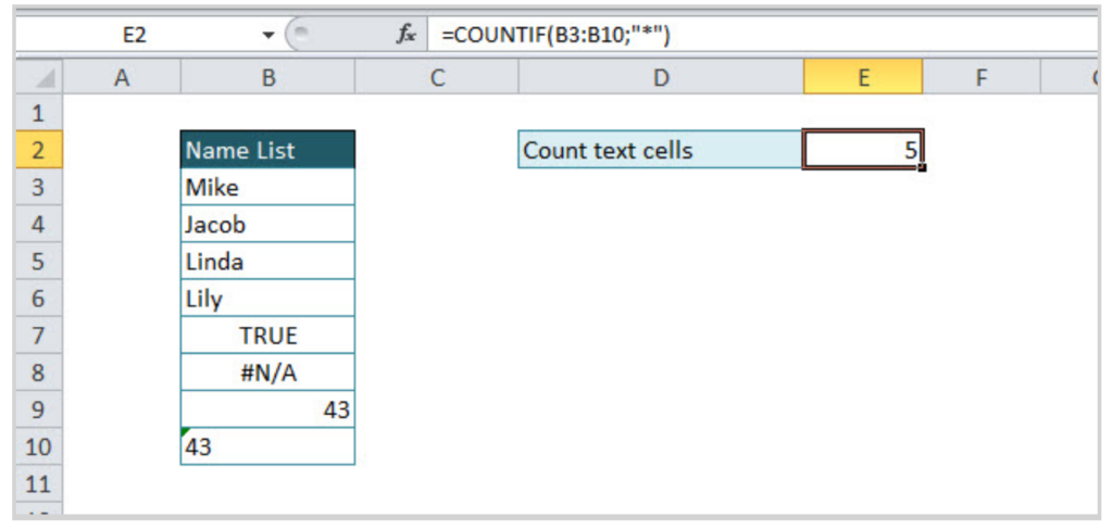
Text Cells can be easily found in Excel using COUNTIF or COUNTIFS functions. The COUNTIF function searches text cells based on specific criteria and in the defined range. As in the example below, the defined range is table Name list, and text criteria is defined using wildcard “*”. The formula result is 5, all text cells have been counted. Note that number formatted as text in cell B10 is also counted, but Booleans (TRUE /FALSE) and error (#N/A) are not recognized as text.
The formula for counting text cells:
=COUNTIF(range;"*")
For counting non-text cells, the formula should be a little bit changed in criteria part:
=COUNTIF(range;"<>*")
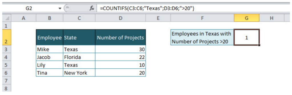
If there are several criteria for counting cells, then COUNTIFS function should be used. For example, if we want to count the number of employees from Texas with project number greater than 20, then the function will look like:
=COUNTIFS(C3:C6;"Texas";D3:D6;">20").
In criteria range in column State, a specific text criteria is defined under quotations “Texas”. The second criteria is numeric, criteria range is column Number of projects, and criteria is numeric value greater than 20, also under quotations “>20”. If we were looking for exact value, the formula would look like:
=COUNTIFS(C3:C6;"Texas";D3:D6;20)
Count Specific Text in Cells
For counting specific text under cells range, COUNTIF function is suitable with the formula:
=COUNTIF(range;"*text*")
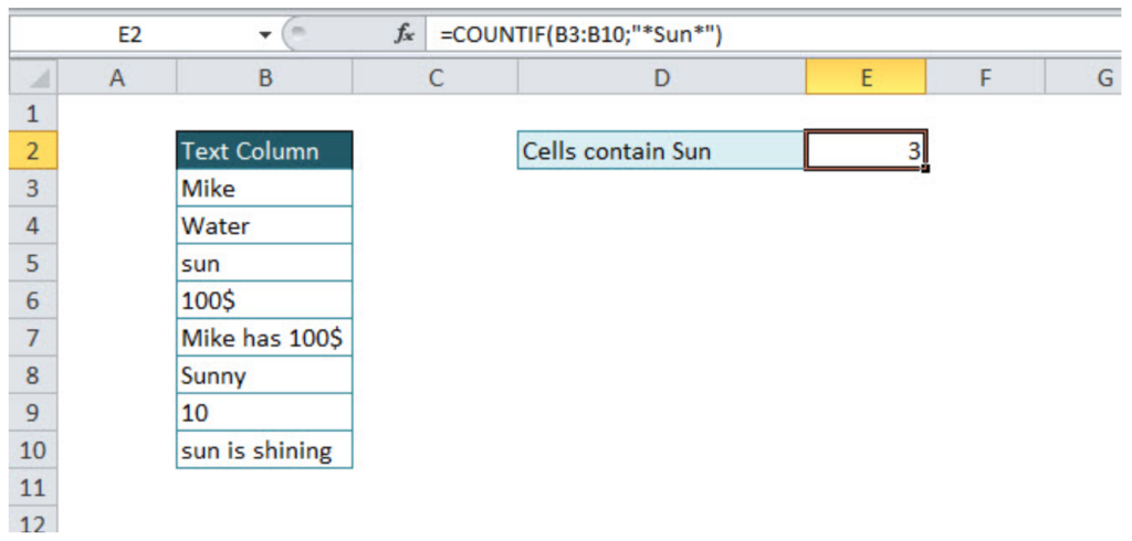
=COUNTIF(B3:B9;"*Mike*")
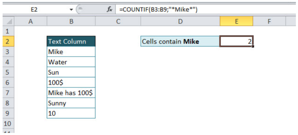
The first part of the formula is range and second is text criteria, in our example “*Mike*”. If wildcard * has not been used before and after criteria text, formula result would have been 1 (Formula would find cells only with word Mike). Wildcard * before and after criteria text, means that all cells that contain criteria characters will be taken into account. As in another example below with text criteria Sun, three cells were found (sun, Sunny, sun is shining)
=COUNTIF(B3:B10;"*Sun*")
Note: The COUNTIF function is not case sensitive, an alternative function for case sensitive text searches is SUMPRODUCT/FIND function combination.
Count Case Sensitive Specific Text
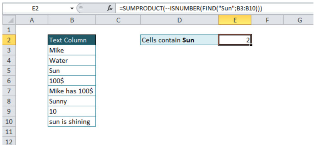
For a case-sensitive text count, a combination of three formulas should be used: SUMPRODUCT, ISNUMBER and FIND. Let’s look in the example below. If we want to count cells that contain text Sun, case sensitive, COUNTIF function would not be the appropriate solution, instead of this function combination of three functions mentioned above has to be used.
=SUMPRODUCT(--ISNUMBER(FIND("Sun";B3:B10)))
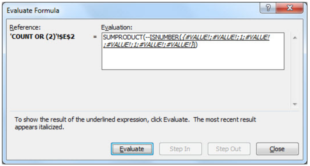
We should go through a separate function explanation in order to understand functions combination. FIND function, searches specific text in the defined cell, and returns the number of the starting position of the text used as criteria. This explanation is relevant, if the searching range is just one cell. If we want to use FIND function in a range of the cells, then the combination with SUMPRODUCT function is necessary.
Without ISNUMBER, function combination of FIND and SUMPRODUCT functions would return an error. ISNUMBER function is necessary because whenever FIND function does not match defined criteria, the output will be an error, as in print screen below of the evaluated formula.
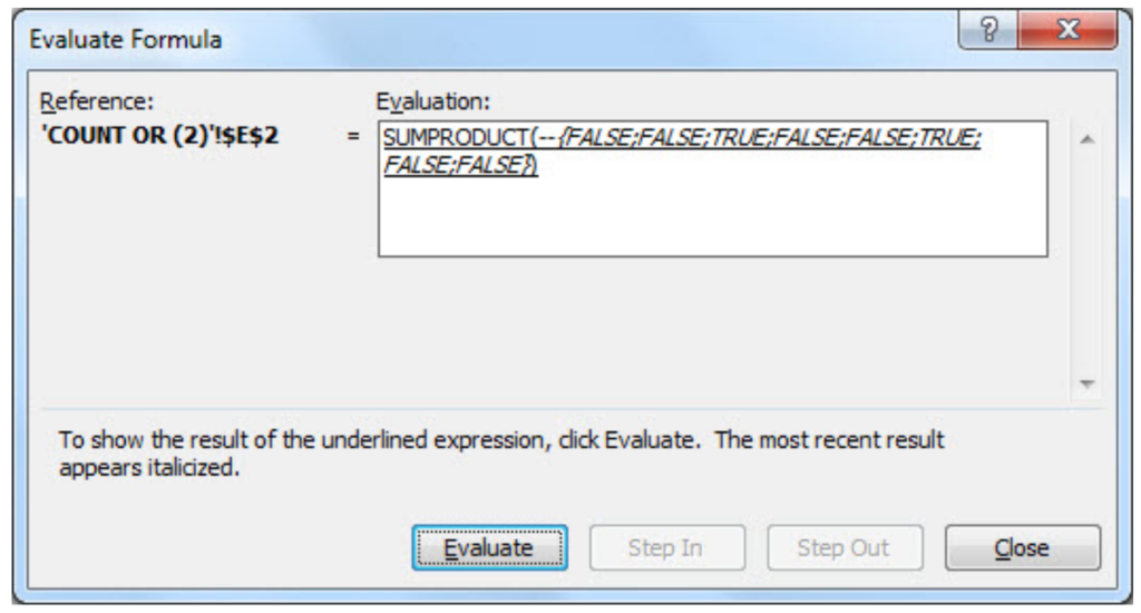
In order to change error values with Boolean TRUE/FALSE statement, ISNUMERIC formula should be used (defining numeric values as TRUE, and non-numeric as FALSE, as in print screen below).
You might be wondering what character — in SUMPRODUCT function stands for. It converts Boolean values TRUE/FALSE in numeric values 1/0, enabling SUMPRODUCT function to deal with numeric operations (without character — in SUMPRODUCT function, the final result would be 0).
Remember, if you want to count specific text cells that are not case sensitive, COUNTIF function is suitable. For all case sensitive searches combination of SUMPRODUCT/ISNUMBER/FIND functions is appropriate.
Count Text Cells with Multiple Criteria
If you want to count cells with Multiple criteria, with all criteria acceptable, there is an interesting way of solving that problem, a combination of SUMPRODUCT/ISNUMBER/FIND functions. Please take a look in the example below. We should count all cells that contain either Mike or $. Tricky part could be the cells that contain both Mike and $.
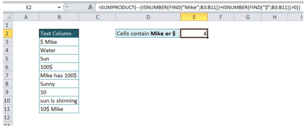
=SUMPRODUCT(--(ISNUMBER(FIND("Mike";B3:B11))+ISNUMBER(FIND("$";B3:B11))>0))
Formula just looks complex, in order to be easier for understanding, I will divide it into several steps. Also, knowledge from the previous tutorial point will be necessary for further work, since the combination of FIND, ISNUMBER, and SUMPRODUCT functions have been explained.
In the first part of the function, we loop through the table and find cells that contain Mike:
=ISNUMBER(FIND("Mike";B3:B11))
The output of this part of the function will be an array with values {1;0;0;0;1;0;0;0;1}, number 1, where criteria have been met, and 0, where has not.
In the second part of the function, looping criteria is $, counting cells containing this value:
=ISNUMBER(FIND("$";B3:B11))
The output of this part of the function will be an array with values {1;0;0;1;1;0;0;0;1}, number 1, where criteria have been met, and 0, where has not.
Next step is to sum these two arrays, since cell should be counted if any of conditions is fulfilled:
=ISNUMBER(FIND("Mike";B3:B11))+ISNUMBER(FIND("$";B3:B11))
The output of this step is {2;0;0;1;2;0;0;0;2}, the number greater than 0 means that one of the condition has been met (2 – both conditions, 1 – one condition)
Without function part >0, the final function would double count cells that met both conditions and the final result would be 7 (sum of all array numbers). In order to avoid it, in the formula should be added >0:
=ISNUMBER(FIND("Mike";B3:B11))+ISNUMBER(FIND("$";B3:B11))>0
The output of this step is array {1;0;0;1;1;0;0;0;1}, the previous array has been checked and only values greater than 0 are TRUE (in an array have value 1), and others are FALSE (in an array have value 0).
Final output of the formula is the sum of the final array values, 4.
Looks very confusing, but after several usages, you will become familiar with this functions.
At the end, we will cover one more multiple criteria text count function, already mentioned in the tutorial, COUNTIFS function. In order to distinguish the usage of functions mentioned above and COUNTIFS function, two words are enough OR/AND. If you want to count text cells with multiple criteria but all conditions have to be met at the same time, then COUNTIFS function is appropriate. If at least one condition should be met, then the combination of function explained above is suitable.
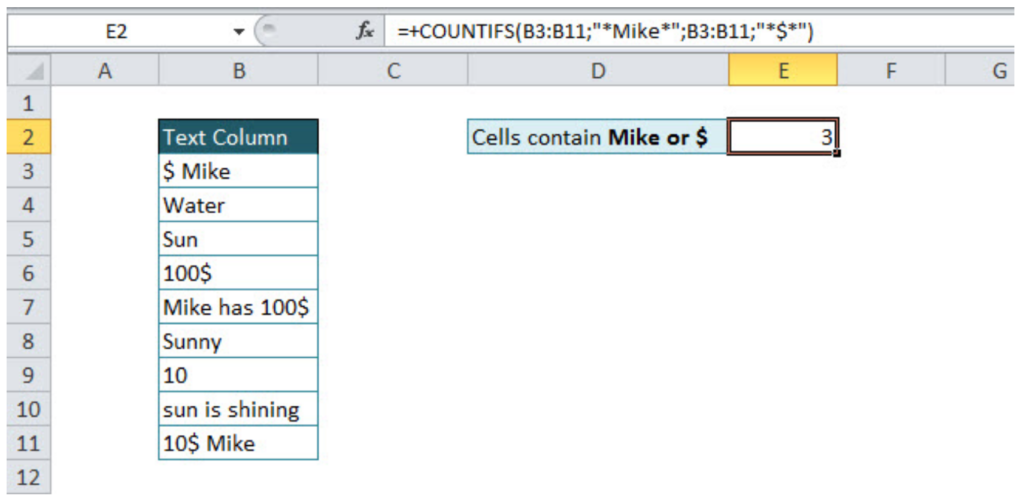
Look at the example below, the number of cells that contain both Mike and $ is easily calculated with COUNTIFS function:
=COUNTIFS(range1;"*text1*";range2;"*text2*")
=COUNTIFS(B3:B11;"*Mike*";B3:B11;"*$*")
In the defined range, function counts only cells where both conditions have been met. The final result is 3.
Still need some help with Excel formatting or have other questions about Excel? Connect with a live Excel expert here for some 1 on 1 help. Your first session is always free.
I am trying to count the number of times a sub-string appears within a column of string data in Excel. Please see the below example.
The column of string data (tweets) looks like this:
   A
1  An example string with @username in it
2  RT @AwesomeUser says @username is awesome
The column with «substrings» (Twitter screen names) looks like this:
   B
1  username
2  AwesomeUser
I want to use a formula to count the number of times that a substring from B1, B2, etc. appears in the strings in column A. For example: a formula searching for B1 would return «2» and a search for B2 would return «1».
I can’t do it this way:
=COUNTIF(A:A, "username")
because COUNTIF only looks for strings, not substrings. This formula would always return «0».
Here’s a formula I thought might do it:
=SUMPRODUCT((LEN(A:A)-(LEN(SUBSTITUTE(A:A,"username",""))))/LEN("username"))
Unfortunately, I have 16,000 entries in column B and tens of thousands in A, so counting characters won’t work even on a high power PC (also, the result returned by the function is suspect).
I thought about using:
=COUNTIF(A:A, "*username*")
but COUNTIF requires a string with the star operators; I need to use cell references due to the volume of data.
My question: does anyone know how I can use a formula for this? If using COUNTIF, how do I get a cell reference in the conditional part of the statement (or use a function to substitute the string in the cell referenced within the conditional part of a COUNTIF statement)?
I know that I could parse the data, but I would like to know how to do it in Excel.
Explanation
In this example, the goal is to count numbers that appear in column B. The COUNT function is designed to only count numeric values, but because all values in the range B5:B15 are text, COUNT will return zero. One approach is to split the characters in each text value into an array, then use the COUNT function to count numbers in the result. This approach is described below.
Create the array
The first step is to split the text string into an array of characters. This is done with MID, LEN, and SEQUENCE like this:
MID(B5,SEQUENCE(LEN(B5)),1)In a nutshell, the LEN function returns the length of the text in B5, which is 9, to the SEQUENCE function as the rows argument. SEQUENCE then generates an a numeric array like {1;2;3;4;5;6;7;8;9}, which is returned to the MID function as the start_num argument:
=MID(B5,{1;2;3;4;5;6;7;8;9},1)The MID function then extracts each of the 9 characters and returns an array like {«1″;»8″;» «;»a»;»p»;»p»;»l»;»e»;»s»}. Read a more detailed explanation here.
Count numbers
Back in the original formula, we use a double-negative (—) operation to force Excel to try and convert each character to a number:
=COUNT(--{"1";"8";" ";"a";"p";"p";"l";"e";"s"})Where this operation succeeds, we get a numeric value. Where it fails, we get a #VALUE! error:
=COUNT({1;8;#VALUE!;#VALUE!;#VALUE!;#VALUE!;#VALUE!;#VALUE!;#VALUE!})The COUNT function then counts the numbers in the array and returns a final result of 2. As the formula is copied down column D, it returns a count of the numbers in each text string in column B.
Legacy Excel
In Legacy Excel, which lacks dynamic arrays and the SEQUENCE function, it is more challenging to split a text string to an array of characters. One workaround is to use the ROW and INDIRECT function like this:
=COUNT(--MID(B5,ROW(INDIRECT("1:"&LEN(B5))),1))The INDIRECT function is a way of creating a valid Excel reference with text. The ROW function then evaluates the text and returns a reference. The reference in this case is 1:9 (rows 1 through 9), and the ROW function then returns an array of corresponding row numbers. The resulting array is the same as with the SEQUENCE function above:
=COUNT(--MID(B5,{1;2;3;4;5;6;7;8;9},1))In the end, this formula returns the same result as above, 2. Note this is an array formula and must be entered with control + shift + enter in older versions of Excel.