
Count characters in cells
Excel for Microsoft 365 Excel for the web Excel 2021 Excel 2019 Excel 2016 Excel 2013 More…Less
When you need to count the characters in cells, use the LEN function—which counts letters, numbers, characters, and all spaces. For example, the length of «It’s 98 degrees today, so I’ll go swimming» (excluding the quotes) is 42 characters—31 letters, 2 numbers, 8 spaces, a comma, and 2 apostrophes.
To use the function, enter =LEN(cell) in the formula bar, then press Enter on your keyboard.
Multiple cells: To apply the same formula to multiple cells, enter the formula in the first cell and then drag the fill handle down (or across) the range of cells.
To get the a total count of all the characters in several cells is to use the SUM functions along with LEN. In this example, the LEN function counts the characters in each cell and the SUM function adds the counts:
=SUM((LEN(
cell1
),LEN(
cell2
),(LEN(
cell3
))
)).
Give it a try
Here are some examples that demonstrate how to use the LEN function.
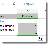
Copy the table below and paste it into cell A1 in an Excel worksheet. Drag the formula from B2 to B4 to see the length of the text in all the cells in column A.
|
Text Strings |
Formulas |
|---|---|
|
The quick brown fox. |
=LEN(A2) |
|
The quick brown fox jumped. |
|
|
The quick brown fox jumped over the lazy dog. |
Count characters in one cell
-
Click cell B2.
-
Enter =LEN(A2).
The formula counts the characters in cell A2, which totals to 27—which includes all spaces and the period at the end of the sentence.
NOTE: LEN counts any spaces after the last character.
Count
characters in
multiple cells
-
Click cell B2.
-
Press Ctrl+C to copy cell B2, then select cells B3 and B4, and then press Ctrl+V to paste its formula into cells B3:B4.
This copies the formula to cells B3 and B4, and the function counts the characters in each cell (20, 27, and 45).
Count a total number of characters
-
In the sample workbook, click cell B6.
-
In the cell, enter =SUM(LEN(A2),LEN(A3),LEN(A4)) and press Enter.
This counts the characters in each of the three cells and totals them (92).
Need more help?
Excel has some amazing text functions that can help you when working with the text data.
In some cases, you may need to calculate the total number of characters in a cell/range or the number of times a specific character occurs in a cell.
While there is the LEN function that can count the number of characters in a cell, you can do the rest as well with a combination of formulas (as we will see later in the examples).
In this tutorial, I will cover different examples where you can count total or specific characters in a cell/range in Excel.
Count All Characters in a Cell
If you simply want to get a total count of all the characters in a cell, you can use the LEN function.
The LEN function takes one argument, which could be the text in double-quotes or the cell reference to a cell that has the text.
For example, suppose you have the dataset as shown below and you want to count the total number of characters in each cell:

Below is the formula that will do this:
=LEN(A2)

By itself, the LEN function may not look like much, but when you combine it with other formulas, it can do some wonderful things (such as get the word count in a cell or split first and last name).
Note: LEN function will count all the characters in a cell, be it a special character, numbers, punctuation marks, and space characters (leading, trailing, and double spaces between words).
Since the LEN function counts every character in a cell, sometimes you may get the wrong result in case you have extra spaces in the cell.
For example, in the below case, the LEN function returns 25 for the text in cell A1, while it should have been 22. But since it’s counting extra space characters as well, you get the wrong result.

To avoid extra spaces being counted, you can first use the TRIM function to remove any leading, trailing and double spaces and then use the LEN function on it to get the real word count.
Below formula will do this:
=LEN(TRIM(A2))

Count All Characters in a Range of Cells
You can also use the LEN function to count the total number of characters in an entire range.
For example, suppose we have the same dataset and this time, instead of getting the number of characters in each cell, I want to know how many are there in the entire range.
You can do that using the below formula:
=SUMPRODUCT(LEN(A2:A7)))

Let me explain how this formula works.
In the above formula, the LEN part of the function takes an entire range of cells and counts the characters in each cell.
The result of the LEN function would be:
{22;21;23;23;23;31}
Each of these numbers represents the character count in the cell.
And when you use the SUMPRODUCT function with it, it would simply add all these numbers.
Now, if you’re wondering why can’t you use SUM instead of SUMPRODUCT, the reason is that this is an array, and SUMPRODUCT can handle array but the SUM function can not.
However, if you still want to use SUM, you can use the below formula (but remember that you need to use the Control + Shift + Enter to get the result instead of a regular Enter)
=SUM(LEN(A2:A7))
Count Specific Characters in a Cell
As I mentioned that the real utility of the LEN function is when it’ used in combination with other formulas.
And if you want to count specific characters in a cell (it could be a letter, number, special character, or space character), you can do that with a formula combination.
For example, suppose you have the dataset as shown below and you want to count the total number of words in each cell.
While there is no in-built formula to get the word count, you can count the space characters and then use it to know the total number of words in the cell.
Below is the formula that will give you the total number of space characters in a cell:
=LEN(A2)-LEN(SUBSTITUTE(A2," ",""))+1

The above formula counts the total number of space characters and then adds 1 to that number to get the word count.
Here is how this formula works:
- SUBSTITUTE function is used to replace all the space characters with a blank. The LEN function is then used to count the total number of characters when there are no space characters.
- The result of the LEN(SUBSTITUTE(A2,” “,””)) is then subtracted from LEN(A2). This gives us the total number of space characters that are there in the cell.
- 1 is added in the formula and the total number of words would be one more than the total number of space characters (as two words are separated with one character).
Note that in case there are any leading, trailing, or double spaces, you are going to get the wrong result. In such a case, it’s best to use the TRIM function along with the LEN function.
You can also use the same logic to find a specific character or word or phrase in a cell.
For example, suppose I have a dataset as shown below where I have different batches, where each batch has an alphabet and number to represent it (such as A1, J2, etc.)

Below is the formula that will give you the total number of times a batch with the alphabet A has been created each month:
=LEN(B2)-LEN(SUBSTITUTE(B2,"A",""))

The above formula again uses the same logic – find the length of the text in a cell with and without the character that you want to count and then take the difference of these two.
In the above formula, I have hardcoded the character that I want to count, but you can also put it in a cell and then use the cell reference. This makes it more convenient as the formula would update the next time you change the text in the cell.
Count Specific Characters Using Case-Insensitive Formula
There is one issue with the formula used to count specific characters in a cell.
The SUBSTITUTE function is case sensitive. This means that you “A” is not equal to “a”. This is why you get the wrong result in cell C5 (the result should have been 3).

So how can you get the character count of a specific character when it could have been in any case (lower or upper).
You do that by making your formula case insensitive. While you can go for a complex formula, I simply added the character count of both the cases (lowercase and uppercase A).
=LEN(B2)-LEN(SUBSTITUTE(B2,"A",""))+LEN(B2)-LEN(SUBSTITUTE(B2,"a",""))

Count Characters/Digits Before and After Decimal
I don’t know why, but this is a common query I get from my readers and have seen in many forums – such as this one
Suppose you have a dataset as shown below and you want to count the characters before the decimal and after the decimal.

Below are the formulas that will do this.
Count characters/numbers before the decimal:
=LEN(INT(A2))
Count characters/numbers after the decimal:
=LEN(A2)-FIND(".",A2)

Note that these formulas are meant only for significant digits in the cell. In case you have leading or trailing zeroes or you have used custom number formatting to show more/fewer numbers, the above formulas would still give you significant digits before and after the decimal.
So these are some of the scenarios where you can use formulas to count characters in a cell or a range of cells in Excel.
I hope you found the tutorial useful!
Other Excel tutorials you may like:
- Count Unique Values in Excel Using COUNTIF Function
- How to Count Cells that Contain Text Strings
- How to Count Colored Cells In Excel
- Count Unique Values in Excel Using COUNTIF Function
- How To Remove Text Before Or After a Specific Character In Excel
While working with Excel, one often needs to count the number of characters in single or multiple cells. Such characters can be numeric, textual or in the form of a special character. To count characters in excel, the LEN function is used either alone or in combination with other functions of Excel. This function counts alphabets, numbers, spaces, special characters, and punctuation marks.
For example, the formula =LEN(“Let’s set the goals for this year.”) returns 34, which includes 26 alphabets, 6 spaces, 1 apostrophe, and 1 period. The quotes within which the text string is enclosed are excluded from the count.
The purpose of counting characters in excel is to ensure that the length of the string does not exceed the word count limitations set for certain worksheets. Moreover, a character count is essential before releasing a brochure, advertisement, business card or Excel report.
Table of contents
- Count Characters in an Excel Cell
- How to Count Characters in Excel?
- Example #1–Count all Characters in Each Cell of a Column
- Example #2–Count the Characters Left in a Cell After Excluding a Specific Character
- Example #3–Count the Occurrence of a Specific Character in a Cell
- Example #4–Count all Characters of a Vertical Range
- Frequently Asked Questions
- Recommended Articles
- How to Count Characters in Excel?
You can download this Count Characters Excel Template here – Count Characters Excel Template
How to Count Characters in Excel?
Let us consider a few examples to understand the technique of counting characters in Excel.
Example #1–Count all Characters in Each Cell of a Column
The succeeding image shows some names in column A. We want to count the number of characters in each cell of the range A2:A15. Use the LEN function of Excel.
The steps to count characters in excel by using the LEN function are listed as follows:
Step 1: Enter the following formula in cell B2.
“=LEN(A2)”
Step 2: Press the “Enter” key. Next, drag the fill handle (bottom-right corner) of cell B2 till cell B15. The formula (of cell B2) and the outputs are shown in the succeeding image.
Hence, the total characters in each cell of column A have been counted and returned in the corresponding cell of column B.
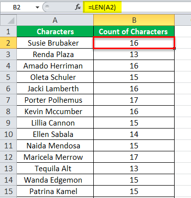
Explanation: Apart from the characters of each name, the count (in column B) includes three spaces. One space is between the first and the last name. The remaining two spaces have been deliberately inserted after the last name in each cell.
Hence, to know only the number of letters of a cell (of column A), one needs to subtract 3 from the respective output (of column B).
Note 1: The syntax of the LEN functionThe Len function returns the length of a given string. It calculates the number of characters in a given string as input. It is a text function in Excel as well as an inbuilt function that can be accessed by typing =LEN( and entering a string as input.read more is “LEN(text).” The “text” is the string whose characters are to be counted. It is a required argument. This argument can either be supplied as a text string within double quotes or as a reference to a cell containing text.
The argument “text” does not mean that the cell should necessarily contain a text string. The LEN function can count any kind of character contained by a cell.
Note 2: The LEN function counts all kinds of spaces, whether leading, trailing, or between the text strings.
Example #2–Count the Characters Left in a Cell After Excluding a Specific Character
Working on the dataset of example #1, we have placed the character “@” between the first and the last names. Count the number of characters in each excel cell of the range A2:A12. The count should exclude the character “@.”
Use the LEN and SUBSTITUTE functions of excel.
The steps to count the number of characters by using the given excel functions are listed as follows:
Step 1: Enter the following formula in cell C2.
“=LEN(SUBSTITUTE(A2,“@”,“”))”
Step 2: Press the “Enter” key. Then, drag the fill handle of cell C2 till cell C12. The formula (of step 1) and the outputs are shown in the following image.
Hence, the length of the string excluding character “@” has been obtained in column C.

Explanation: In the given formula (entered in step 1), the SUBSTITUTE functionSubstitute function in excel is a very useful function which is used to replace or substitute a given text with another text in a given cell, this function is widely used when we send massive emails or messages in a bulk, instead of creating separate text for every user we use substitute function to replace the information.read more is processed first, followed by the LEN function. This formula works as follows:
- The SUBSTITUTE function replaces the character “@” with an empty string. An empty string is represented by a pair of double quotation marks (like “”).
- Next, the LEN function realizes that the character “@” has been excluded from each cell of column A. Consequently, it counts the characters left after such exclusion.
Notice that each output of column C is one less than the corresponding output of column B. This is because, in column B, the LEN function has counted a space between the first and the last names (refer to the “explanation” of example #1). This space has been replaced by the character “@” in the current example. Further, this single character is excluded from the count.
Note 1: The syntax of the SUBSTITUTE function is shown in the following image.
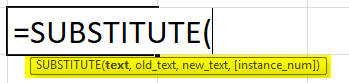
The “text” argument is the text string (or the reference to a cell containing text) in which characters need to be substituted. The “old_text” is the text to be replaced. The “new_text” is the text with which replacement has to be carried out. The “instance_num,” being an optional argument, indicates which occurrence of the “old_text” should be replaced by the “new_text.”
Note 2: In the current example, the reference “A2” is the “text” argument of the SUBSTITUTE function. The “old_text” argument is “@” and the “new_text” argument is an empty string (“”). Since the “instance_num” argument has been omitted, every occurrence of the “old_text” has been replaced with “new_text.”
At present, there is only one occurrence of “@” in each name (of column A). Had there been multiple occurrences of this character in a single name, all instances would have been excluded from the count by the LEN function (as “instance_num” is omitted).
Note 3: The SUBSTITUTE function can be used with numbers too. However, remember that the SUBSTITUTE is a case-sensitive function. This means that “A” and “a” are treated differently. For more details related to the SUBSTITUTE function, click the hyperlink given in the explanation of this example.
Example #3–Count the Occurrence of a Specific Character in a Cell
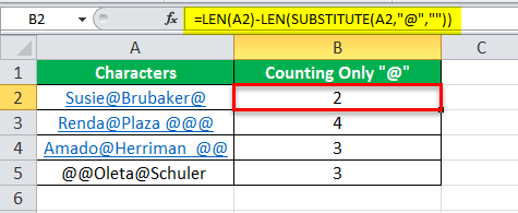
Working on the dataset of example #1, we have inserted character “@” multiple times in four names of column A. Count the number of occurrences of this character in each cell of the range A2:A5.
Use the LEN and SUBSTITUTE functions of Excel.
The steps to count the number of occurrences of the given character are listed as follows:
Step 1: Enter the following formula in cell B2.
“=LEN(A2)-LEN(SUBSTITUTE(A2,“@”,“”))”
Step 2: Press the “Enter” key. Next, drag the formula of cell B2 till cell B5. The formula (of step 1) and the outputs are shown in the following image.
Hence, the number of occurrences of character “@” (in each cell of column A) has been obtained in column B.
Explanation: In the given formula (entered in step 1), we have subtracted the count of characters excluding “@” from the total length of the string.
The count excluding “@” is assessed by the formula “LEN(SUBSTITUTE(A2,“@”,“”).” The count of the entire string is computed by the formula “LEN(A2).” So, when the former is subtracted from the latter, we obtain the count of the character “@.”
Hence, in cell A2, the character “@” appears twice. Likewise, in cell A3, this character appears four times. Irrespective of the placement of this character, it has been counted by the LEN and SUBSTITUTE formula.
Note: For the syntax of the SUBSTITUTE formula, refer to “note 1” given at the end of example #2.
Example #4–Count all Characters of a Vertical Range
Working on the dataset of example #1, we want to sum the characters of the entire range A2:A10. Use the SUMPRODUCT and LEN functions of Excel.
The steps to count the characters of the entire excel range (A2:A10) are listed as follows:
Step 1: Enter the following formula in cell B13.
“=SUMPRODUCT(LEN(A2:A10))”
Step 2: Press the “Enter” key. The formula and the resulting output are shown in the following image.
Hence, the sum of characters of the entire range (A2:A10) is 138.

Explanation: The LEN function alone cannot handle arrays. So, we have enclosed the LEN within the SUMPRODUCT (in step 1) to sum the characters of the entire range (A2:A10).
The formula, entered in step 1, works as follows:
- The LEN function counts the number of characters in each cell of the range A2:A10. This count is returned by the function as an array of numbers.
- The SUMPRODUCT sums the array returned by the LEN function. So, the array of 9 numbers {16,13,16,15,16,17,16,15,14} is summed up by the SUMPRODUCT function.
Notice that the two trailing spaces (after each name) in each cell of the given range have also been counted by the LEN function.
To cross-check the final output returned by the LEN and SUMPRODUCT formulaThe SUMPRODUCT excel function multiplies the numbers of two or more arrays and sums up the resulting products.read more (entered in step 1), one can add the individual outputs given in the range B2:B10. The sum of values of the range B2:B10 is 138.
Note 1: The syntax of the SUMPRODUCT function is shown in the following image.
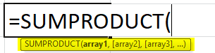
The arguments “array1,” “array2,” “array3,” etc., are the arrays whose values need to be multiplied and then added. “Array1” is required, while the remaining “array” arguments are optional. When a single array is specified, the SUMPRODUCT returns the sum of the values of that array.
Note 2: Alternatively, one can sum the characters of the range A2:A10 by using the formula “=SUM(LEN(A2:A10)).” Enter this formula without the beginning and ending double quotation marks. Once entered, press the keys “Ctrl+Shift+Enter” together.
Frequently Asked Questions
1. What does it mean to count characters and how is it done in Excel?
Each cell of a dataset contains some value that can be numeric, textual or in the form of a special character. One may often need to count these characters (or values) either in certain cells or in the entire dataset.
For counting all characters in a cell of Excel, the LEN function is used. The cell reference, whose characters are to be counted, is supplied to this function as an argument. For counting characters in a range of Excel, the LEN is used in combination with the SUM or the SUMPRODUCT functions of Excel.
Note: For more details related to the syntax and usage of the LEN function, refer to the examples of this article.
2. How to count characters by including and excluding spaces of a cell of Excel?
To count characters by including spaces, use the following formula in Excel:
“=LEN(cell)”
This formula counts all characters of a cell including every space. So, all spaces, whether leading, trailing, or between the words, are counted.
To count characters by excluding spaces, use the following formula in Excel:
“=LEN(SUBSTITUTE(cell,“ ”,“”))”
In this formula, the SUBSTITUTE function replaces all space characters (“ ”) of a cell with an empty text string (“”). Next, the LEN function understands that the spaces have been removed. So, it counts all characters excluding the spaces.
Note: In both the preceding formulas, the argument “cell” is the reference to a cell whose characters are to be counted. When the same cell reference is provided in both formulas and the second formula is subtracted from the first, the count of the space character (in the supplied cell) is obtained.
3. How to count characters in a row of Excel?
The characters of an Excel row can be counted with either of the following formulas:
a. “=SUMPRODUCT(LEN(A1:D1))”
b. “=SUM(LEN(A1:D1))”
After entering the formula in pointer “a,” press the “Enter” key. After entering the formula in pointer “b,” press the keys “Ctrl+Shift+Enter” together.
In both the preceding formulas, the characters of row 1 (from column A to D) have been added. Likewise, to count characters of a column (like column A), enter the respective range (like A1:A4) in any of the given formulas.
Recommended Articles
This has been a guide to counting characters in a cell of Excel. Here we discuss how to count the total characters in an Excel cell by using LEN, SUBSTITUTE, and SUMPRODUCT functions along with Excel examples and downloadable Excel templates. You may also look at these useful functions in Excel–
- Excel Formula for Grade
- Char In Excel
- REPLACE Function in Excel
- TEXT Formula in Excel
- Excel Worksheet Tab
Let’s learn how to count the number of characters in Excel. The count could be performed on a single cell and even a range of cells. While learning that, let’s also shed some light on counting specific characters too. This tutorial will teach you all that is mentioned above using the LEN function with different combos of the SUBSTITUTE, SUMPRODUCT, and SUM functions, working together to do all the monotonous counting for you.
Counting characters or words will at its most be helpful from a designing point of view; How many characters are going onto a business card, the number of words going on a brochure, how many characters will fit according to the size of the object, the font, the design. Having it all counted and sorted gives good perspective!
As for specific embedded characters, you may be looking for certain products via product code, a text symbol that signifies a characteristic, etc. However important or inane your reason, we will find out how to count characters in Excel nonetheless so let’s get counting!
 1")
Count Characters In Excel
We will begin with counting the number of characters in Excel. The example we will use is of inside messages in greeting cards. Depending on the size and design of the greeting card, you will have to see which message can fit where. Hence, it will be helpful to see how many characters a message contains. Below is the example sheet:
 2")
We will go through on how to count characters in a cell and in a range with the LEN function, which you will be seeing a lot of today.
Count Characters in a Cell
Counting characters in excel can be easily done by using the LEN function. The LEN function returns the number of characters in a text string. Let’s see how that pans out:
Here is the formula we will use to count the number of characters in a cell:
=LEN(C4)
And here is what the applied formula looks like:
 3")
The LEN function has been used with a single argument; the reference to the cell for counting the characters in the cell’s text. LEN returns 76 as the number of characters in C4. This count includes space characters. If you want your count to exclude space characters, we’ve got you covered. Read the next segment.
Count Characters in a Cell without Space Characters
If you want the count of the number of characters without space characters, we can slip the SUBSTITUTE function in the LEN function. The SUBSTITUTE function replaces existing text with new text in a text string. The space characters will be swapped for empty text so that the LEN function won’t count the spaces. The formula will look like this:
=LEN(SUBSTITUTE(C4," ",""))
The SUBSTITUTE function replaces the space characters (» «) in C4 with empty text («»). This way, the text that will be left for the LEN function to count will be Maythisbirthdaybejustthebeginningofayearfilledwithhappymemories. The LEN function returns the counted characters as the outcome.
 4")
Count Characters in a Range
If we are to count the number of characters in a range, we may follow something along the lines of adding the individual totals up like:
=LEN(C4)+LEN(C5)+LEN(C6)
But while we’re at it, let’s further explore the potential of the LEN function, shall we? We will now show you how to count the number of characters in a range using the LEN and SUMPRODUCT functions and also the LEN and SUM functions together.
LEN with SUMPRODUCT
Here we will combine the LEN and SUMPRODUCT functions to get a total count of characters in a range. The SUMPRODUCT function calculates the products of ranges and then the sum of the products. Further, we are using the SUMPRODUCT function for summing the LEN function’s count as LEN does not calculate arrays on its own. We have 2 formulas below; one counts characters in the range including space characters, the other excludes space characters:
With spaces:
=SUMPRODUCT(LEN(C4:C6))
The SUMPRODUCT function is used as a helping hand for the LEN function to operate as an array formula. The job of the LEN function is to calculate the total number of characters in the cells C4:C6 which we sum up using the SUMPRODUCT function.
 5")
Without spaces:
=SUMPRODUCT(LEN(SUBSTITUTE(C4:C6," ","")))
Before the LEN and SUMPRODUCT functions get to do their job, the SUBSTITUTE function is used to replace the space characters from C4:C6 with empty characters. The text strings in C4:C6 will then be considered to be without any space characters.
Then the LEN function continues to count the characters and the SUMPRODUCT function sums the values to return 203 as the result.
 6")
LEN with SUM
Instinctively the first function that comes to mind for summations is the SUM function and it works just fine with the LEN function too. In fact, it works just like the SUMPRODUCT function above with a small difference. SUMPRODUCT makes the formula work as an array formula but with LEN and SUM, you need to enclose the formula in curly braces to force the formula into an array formula. Let’s see how to do that using the formula below:
With spaces:
=SUM(LEN(C4:C6))
Once the formula is added, press the Ctrl + Shift + Enter keys and you will notice curly braces bracketing the formula. This turns it into an array formula so that the LEN function can count the characters in C4:C6 as an array with the SUM function.
 7")
Without spaces:
=SUM(LEN(SUBSTITUTE(C4:C6," ","")))
To exclude space characters from the count, we have nested the SUBSTITUTE function to replace all the space characters with empty text. This will leave only letters, numbers, and symbols to be counted. The LEN function counts the characters of each of the cells in C4:C6, the results added by the SUM function. The formula is topped off in the end by hitting the Ctrl + Shift + Enter keys to operate as an array formula and here are the results:
 8")
If you’re wondering what happens if the formula isn’t changed into an array formula, you can try and see the result without adding the curly braces. The formula will only return the count of a single cell; the cell that the result is adjacent to, despite the range present in the formula. The curly braces turn it into an array formula so that it can accept the supplied range.
Recommended Reading: Count Non-Blanks cells from a Range
Count Occurrences of a Specific Character
Sometimes you may need to count out a specific character to differentiate some items from others in the list. You could be looking for certain text, numeric code, or a symbol. We will guide you through counting occurrences of a specific character in a cell and in a range and these are methods you can turn towards when sorting and filtering fail you.
Count Occurrences of a Specific Character in a Cell
As an example, we are looking for products in a dataset that are marked down by an asterisk (*). The marked products will show 1 in the results and the unmarked will show 0. We will use the LEN function for the counting and the SUBSTITUTE function for replacing the text. Let’s put it into Excel action. The formula will be:
=LEN(C3)-LEN(SUBSTITUTE(C3,"*",""))
Using the SUBSTITUTE function, we are replacing the asterisk in C3 with empty text and counting the remnant characters with the LEN function. That brings 7 characters as the count.
It sounds a little questionable up until this point but then we subtract this count from the total character count of C3 which is 8 characters. 8-7=1 which is the result, confirming that C3 does contain an asterisk.
All the codes in our example are 7 characters and a cell not containing an asterisk will compute as 7-7=0.
 9")
All the products resulting in 1 from the formula are the marked products and 0s are the unmarked products.
Count Occurrences of a Specific Character in a Range
Utilizing a formula similar to the one used for counting a specific character in a cell, we will put the SUMPRODUCT function and a range into the works to arrive at the count of a specific character in a range. This means we will be using the LEN and SUBSTITUTE functions again along with the SUMPRODUCT function to bring everything together. The formula put together is:
=SUMPRODUCT(LEN(C3:C18)-LEN(SUBSTITUTE(C3:C18,"*","")))
We can use the above formula in our example to find out how many products have been marked with an asterisk. In the formula, all the asterisks in the range C3:C18 have been substituted with empty text by the SUBSTITUTE function. The LEN function counts all the characters in C3:C18 (excluding the asterisks) which would amount to 16 products multiplied by 7-character code, which equals 112 characters.
In the LEN(C3:C18)-LEN(SUBSTITUTE(C3:C18,»*»,»»)) part of the function, the count of 112 is subtracted from the total character count of C3:C18. If we do a quick check of the total count in the sheet, it amounts to 122 characters. 122-112=10 is the outcome of the formula.
But where does the SUMPRODUCT function come in all of this? SUMPRODUCT is the function working to collate the results of the range in the formula and also works to make the LEN function operate as an array formula.
 10")
Therefore, we have 10 marked products in our dataset.
Counting down to a characteristic close. Today the LEN function has been quite the friend we can count on (count with, actually). Try using some of these methods next time when faced with something as meticulous as character counting; no one should have to do that alone. And making sure you’re never so forlorn in your Excel adventures, we’ll be back with another facet to explore.
After this tutorial you will be able to count total characters in a cell or range, occurrences of specific character or character combination in a cell or range with both case sensitive and insensitive alternatives. Knowledge gained in this tutorial is a really good base for further creative Excel problem-solving.
How to Count Characters in Excel
If you want to learn how to count characters in Excel, you need to use function LEN, using formula =LEN(cell) for counting total characters in a cell, or combination of functions SUMPRODUCT and LEN for counting total characters in a range with formula =SUMPRODUCT(LEN(range)). Additionally, counting of a specific character in a cell or range and specific combination of characters in a cell or a range will be explained in detail.
- Count Total Characters in a Cell
- Count Total Characters in a Range
- Count Specific Character in a Cell
- Count Specific Character in a Range
- Count Specific Combination of Characters in a Cell or Range
Count Total Characters in a Cell
Total characters in a cell can be easily found using Excel function LEN. This function has only one argument, cell reference or text, where total character number would like to be counted:
=LEN(text)
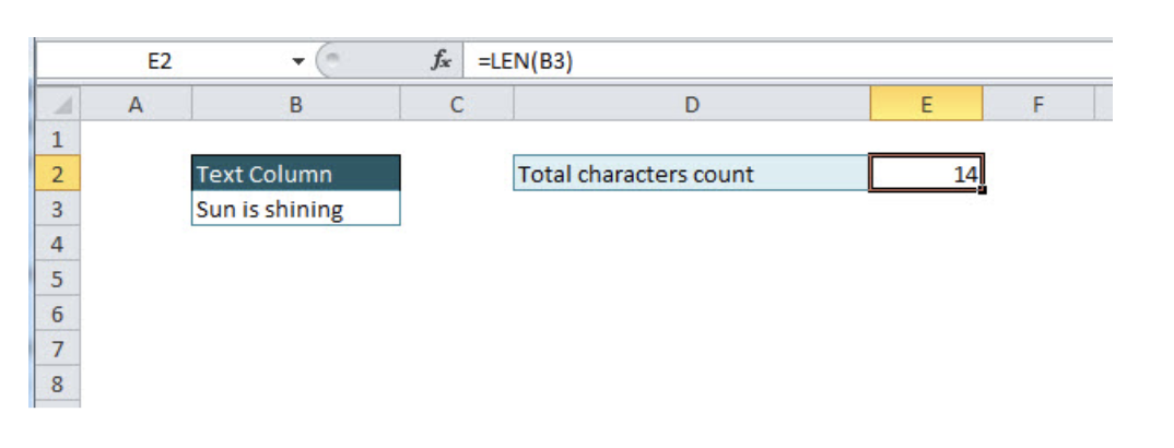
=LEN(B3)
This function counts total characters in a cell, including spaces, punctuation marks, symbols, despite how many times they occur in a string.
If we want to count total characters in a cell, excluding spaces, the combination of formulas LEN and SUBSTITUTE will be required. Let’s take a look in the example below, the formula that excludes spaces looks like:
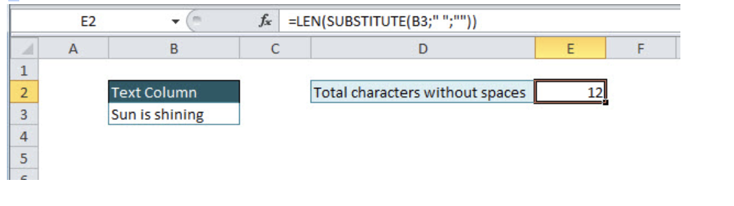
=LEN(SUBSTITUTE(B3;" ";""))
The SUBSTITUTE function changes in a defined cell one character/text with another character/text. If we want to exclude spaces, using this function, they will be eliminated, replacing all occurrences of spaces with an empty string. After SUBSTITUTE, function text in a cell would look like:
=LEN(“Sunisshining”)
After that, it is easy to count total characters with LEN function, with the final result of 12 characters.
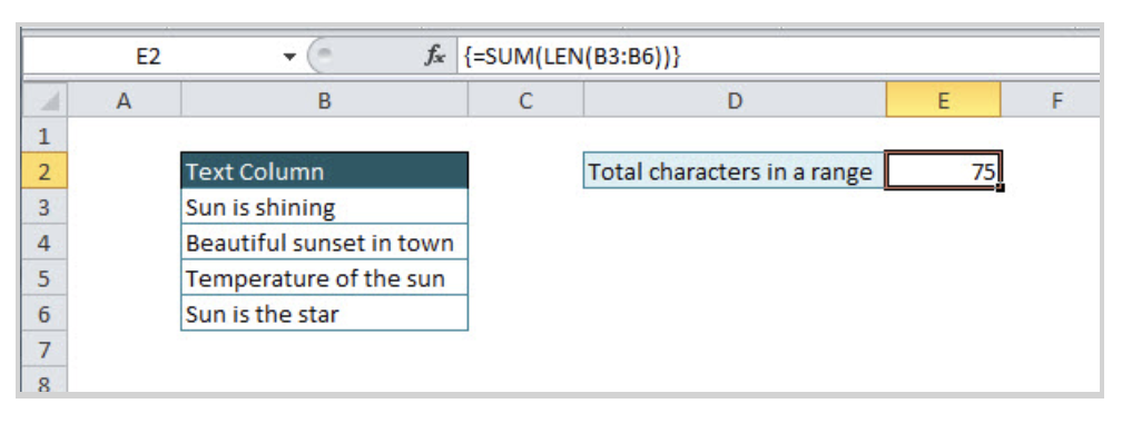
Count Total Characters in a Range
For counting total character number in a defined range, the combination of two functions is needed, SUMPRODUCT and LEN. SUMPRODUCT function usage is elegant solution whenever we are dealing with multiple cells or arrays. Take a look in the example below and a combination of the formulas:
=SUMPRODUCT(LEN(range))
=SUMPRODUCT(LEN(B3:B6))
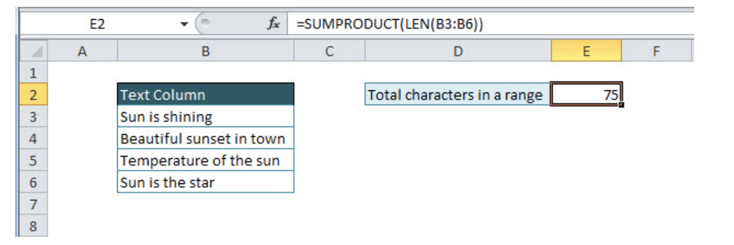
LEN function is related to cell, but for cell ranges usage of summed LEN functions (=LEN(B3)+LEN(B4)+LEN(B5)+LEN(B6)) is not the best solution since we could be dealing with huge ranges. Instead of that, SUMPRODUCT function summarizes results of LEN function in the defined range. In formula evaluation, the result will look like:
=SUMPRODUCT({14;24;22;15})
Numbers from the array are LEN function results from each cell in the defined range B3:B6, giving final character results of 75.
The alternative solution for dealing with ranges is the usage of SUM and LEN function combination. The syntax is almost the same, with the only difference of curly brackets usage, in order to convert SUM function in array formula (Shortcut for creating an array is CTRL+SHIFT+ENTER). In the formula below is the exact syntax for SUM/LEN function combination:
={SUM(LEN(B3:B6))}
Count Specific Character in a Cell
Besides the total character number, there is also the option in Excel for counting the number of occurrences of specific characters. Let’s go through the example of counting number of single character in a specific cell. For this purpose combination of LEN and SUBSTITUTE function is needed, as we did in the similar example of counting the number of characters in the cell without space. Formula syntax will look like:
=LEN(cell)-LEN(SUBSTITUTE(cell;character;""))
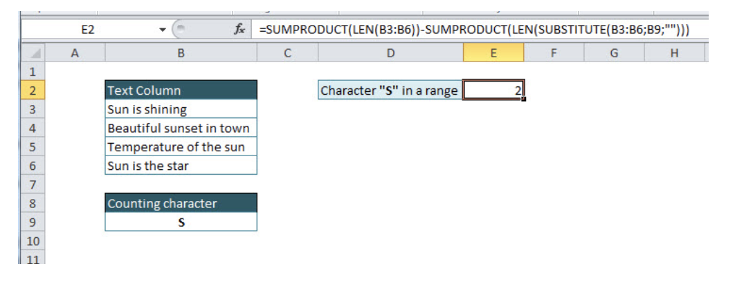
In a specific example, if we want to count the number of character s in a defined cell B3, the formula will look like:
=LEN(B3)-LEN(SUBSTITUTE(B3;"s";""))
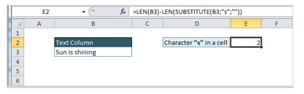
Let’s explain briefly logic of the function combination. Total character number in a cell B3 is subtracted with character number in the same cell, but without specific character that we want to count. As mentioned in tutorial point 1, SUBSTITUTE function is used to change a string in a defined cell in form without specific character, replacing that character with an empty string.
=SUBSTITUTE(cell;"character";"")
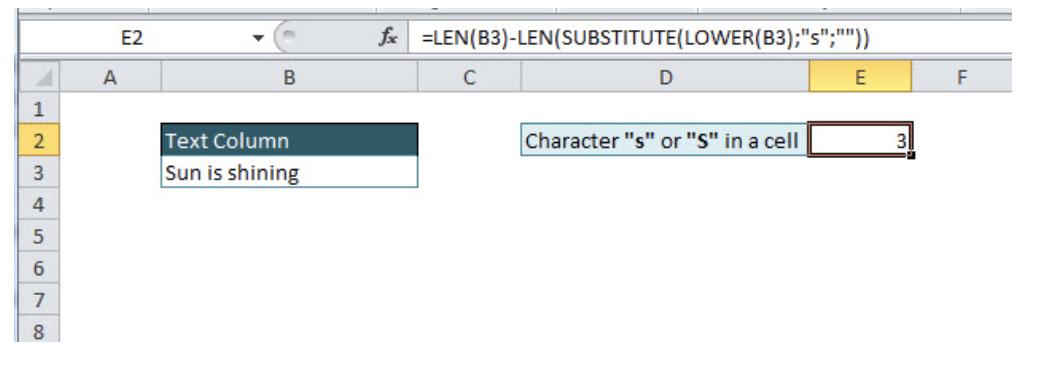
It can be noticed in the final result that function is not counting uppercase characters since LEN function is case sensitive. The solution for counting characters without case sensitive criteria is the usage of UPPER/LOWER function, where all characters will be translated to uppercase/lowercase and function will become case-insensitive.
In the example below, function LOWER is nested into SUBSTITUTE function, changing all string in cell B3 into lowercase, since criteria are defined as lowercase, “s”:
=LEN(cell)-LEN(SUBSTITUTE(LOWER(cell);"lowercase character";""))
=LEN(B3)-LEN(SUBSTITUTE(LOWER(B3);"s";""))
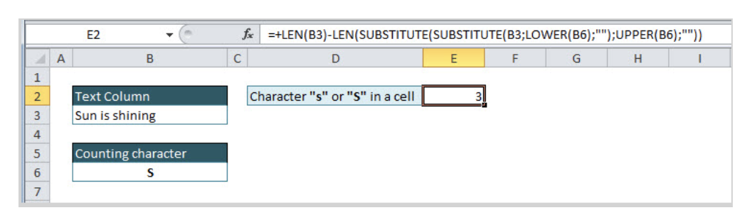
Another solution for making non-case sensitive function is the usage of double nested SUBSTITUTE function in combination with LEN function. In the further example, counting character will be in a specific cell, because sometimes it is not practical to write each time to count a character in the formula, especially if you are dealing with complex ranges and formulas.
Formula with double nested SUBSTITUTE function:
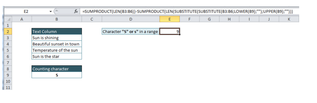
=LEN(cell)-LEN(SUBSTITUTE(SUBSTITUTE(cell;LOWER(character);"");UPPER(character);""))
=LEN(B3)-LEN(SUBSTITUTE(SUBSTITUTE(B3;LOWER(B6);"");UPPER(B6);""))
The formula might be looking complex, but everything will be clear after explanation. Let’s evaluate formula step by step.
First, we want to eliminate the lowercase counting character from the text:
=SUBSTITUTE(B3;LOWER(B6);"")
=SUBSTITUTE(“Sun is shining ”;LOWER(“S”);"")
Function LOWER is put in order to translate counting character into lowercase, and then the +SUBSTITUTE function replaces lowercase character into an empty string. After this step formula result look like: “Sun i hining”.
In the next formula step, the goal is to eliminate the uppercase counting character from the defined text/cell. This is solved by nested SUBSTITUTE function:
=SUBSTITUTE(SUBSTITUTE(B3;LOWER(B6);"");UPPER(B6);"")
We have already explained inside SUBSTITUTE function result “Sun i hining”, and will put it in the function below to make the situation clearer. In first SUBSTITUTE function lowercase character has been replaced with an empty string, and in the second SUBSTITUTE function uppercase counting character is replaced with an empty string, resulting in the text without counting characters “s” and “S”: “un i hining”.
=SUBSTITUTE(“Sun i hining”;UPPER(“S”);"")
LEN function then just counts the number of characters from a modified text:
=LEN(SUBSTITUTE(SUBSTITUTE(B3;LOWER(B6);"");UPPER(B6);""))
=LEN(“un i hining”)
In the final step, evaluated formula result, text without “s” and “S”, is subtracted by the total number of characters in a defined cell:
=LEN(B3)-LEN(SUBSTITUTE(SUBSTITUTE(B3;LOWER(B6);"");UPPER(B6);""))
=LEN(“Sun is shining”) - LEN(“un i hining”)
Count Specific Character in a Range
Whenever we are dealing with cell ranges and arrays, SUMPRODUCT function is needed in combination with other functions. For counting the specific character in a range, for case, sensitive counting, the combination of three functions is used: SUMPRODUCT, LEN, and SUBSTITUTE. For case-insensitive counting, additional formulas should be added: UPPER/LOWER.
First, we will explain counting the number of occurrence of character “S” in a defined range (case insensitive version). A formula is almost similar to formula explaining counting characters. The difference is coming from LEN function nested in SUMPRODUCT function and in counting area, instead of the cell is defined range of cells:
=SUMPRODUCT(LEN(B3:B6))-SUMPRODUCT(LEN(SUBSTITUTE(B3:B6;B9;"")))
For case-insensitive character counting in a defined range, we can use the detailed explained function for case-insensitive character counting in a specific cell in tutorial point 3, with two changes: nesting LEN function in SUMPRODUCT function, and replacing the cell with cell range:
=SUMPRODUCT(LEN(B3:B6))-SUMPRODUCT(LEN(SUBSTITUTE(SUBSTITUTE(B3:B6;LOWER(B9);"");UPPER(B9);"")))
Remember, whenever you are dealing with cell ranges, you will have to use SUMPRODUCT function. For case-sensitive character counting in range combination of functions is needed: SUMPRODUCT, LEN and SUBSTITUTE, and for case-insensitive counting: SUMPRODUCT, LEN, SUBSTITUTE, and UPPER/LOWER functions.
Count Specific Combination of Characters in a Cell or Range
There is also the possibility to count specific character combination in a defined cell or range. In previous tutorial points, we covered single character counting in a cell or range with case sensitive/insensitive alternatives. The formula for counting the combination of characters is the same, only we have to divide it with the number of characters in the character combination.
Let’s take a look in the example below, for counting specific combination of characters in a cell (case insensitive version):
=(LEN(B3)-LEN(SUBSTITUTE(SUBSTITUTE(B3;LOWER(B6);"");UPPER(B6);"")))/LEN(B6)
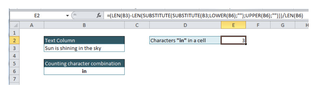
Logic is the same as for counting single character, only we had to divide regular formula with the number of specific characters that we are counting, easily using the formula: LEN(“in”). Without dividing formula with LEN(“in”), the result would be multiplied with the number of characters in character combination (in our example with 2, since “in” has two characters)
For counting specific combination of characters in a cell (case sensitive version) formula will look like:
=(LEN(B3)-LEN(SUBSTITUTE(B3;B6;"")))/LEN(B6)
Counting combination of characters in a range has the same logic as counting single character, and for the case, sensitive version formula will look like:
=(SUMPRODUCT(LEN(B3:B6))-SUMPRODUCT(LEN(SUBSTITUTE(SUBSTITUTE(B3:B6;LOWER(B9);"");UPPER(B9);""))))/LEN(B9)
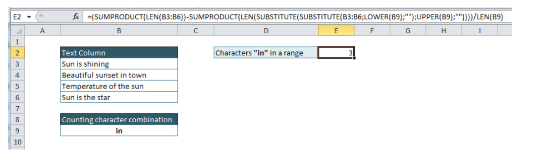
Regular formula explained in tutorials topic 4, is divided with the number of specific characters that we are counting, using function LEN.
If we want the case-insensitive version, then formula syntax will look like:
=(SUMPRODUCT(LEN(B3:B6))-SUMPRODUCT(LEN(SUBSTITUTE(B3:B6;B9;""))))/LEN(B9)
Still need some help with Excel formatting or have other questions about Excel? Connect with a live Excel expert here for some 1 on 1 help. Your first session is always free.