Count of cells with value excel

COUNTIF function

Use COUNTIF, one of the statistical functions, to count the number of cells that meet a criterion; for example, to count the number of times a particular city appears in a customer list.

In its simplest form, COUNTIF says:

• =COUNTIF(Where do you want to look?, What do you want to look for?)

For example:

• =COUNTIF(A2:A5,»London»)

• =COUNTIF(A2:A5,A4)

COUNTIF(range, criteria)

Argument name	Description
range    (required)	The group of cells you want to count. Range can contain numbers, arrays, a named range, or references that contain numbers. Blank and text values are ignored. Learn how to select ranges in a worksheet.
criteria    (required)	A number, expression, cell reference, or text string that determines which cells will be counted. For example, you can use a number like 32, a comparison like «>32», a cell like B4, or a word like «apples». COUNTIF uses only a single criteria. Use COUNTIFS if you want to use multiple criteria.

Examples

To use these examples in Excel, copy the data in the table below, and paste it in cell A1 of a new worksheet.

Data	Data
apples	32
oranges	54
peaches	75
apples	86
Formula	Description
=COUNTIF(A2:A5,»apples»)	Counts the number of cells with apples in cells A2 through A5. The result is 2.
=COUNTIF(A2:A5,A4)	Counts the number of cells with peaches (the value in A4) in cells A2 through A5. The result is 1.
=COUNTIF(A2:A5,A2)+COUNTIF(A2:A5,A3)	Counts the number of apples (the value in A2), and oranges (the value in A3) in cells A2 through A5. The result is 3. This formula uses COUNTIF twice to specify multiple criteria, one criteria per expression. You could also use the COUNTIFS function.
=COUNTIF(B2:B5,»>55″)	Counts the number of cells with a value greater than 55 in cells B2 through B5. The result is 2.
=COUNTIF(B2:B5,»<>»&B4)	Counts the number of cells with a value not equal to 75 in cells B2 through B5. The ampersand (&) merges the comparison operator for not equal to (<>) and the value in B4 to read =COUNTIF(B2:B5,»<>75″). The result is 3.
=COUNTIF(B2:B5,»>=32″)-COUNTIF(B2:B5,»<=85″)	Counts the number of cells with a value greater than (>) or equal to (=) 32 and less than (<) or equal to (=) 85 in cells B2 through B5. The result is 1.
=COUNTIF(A2:A5,»*»)	Counts the number of cells containing any text in cells A2 through A5. The asterisk (*) is used as the wildcard character to match any character. The result is 4.
=COUNTIF(A2:A5,»?????es»)	Counts the number of cells that have exactly 7 characters, and end with the letters «es» in cells A2 through A5. The question mark (?) is used as the wildcard character to match individual characters. The result is 2.

Common Problems

Problem	What went wrong
Wrong value returned for long strings.	The COUNTIF function returns incorrect results when you use it to match strings longer than 255 characters. To match strings longer than 255 characters, use the CONCATENATE function or the concatenate operator &. For example, =COUNTIF(A2:A5,»long string»&»another long string»).
No value returned when you expect a value.	Be sure to enclose the criteria argument in quotes.
A COUNTIF formula receives a #VALUE! error when referring to another worksheet.	This error occurs when the formula that contains the function refers to cells or a range in a closed workbook and the cells are calculated. For this feature to work, the other workbook must be open.

Best practices

Do this	Why
Be aware that COUNTIF ignores upper and lower case in text strings.	Criteria aren’t case sensitive. In other words, the string «apples» and the string «APPLES» will match the same cells.
Use wildcard characters.	Wildcard characters —the question mark (?) and asterisk (*)—can be used in criteria. A question mark matches any single character. An asterisk matches any sequence of characters. If you want to find an actual question mark or asterisk, type a tilde (~) in front of the character. For example, =COUNTIF(A2:A5,»apple?») will count all instances of «apple» with a last letter that could vary.
Make sure your data doesn’t contain erroneous characters.	When counting text values, make sure the data doesn’t contain leading spaces, trailing spaces, inconsistent use of straight and curly quotation marks, or nonprinting characters. In these cases, COUNTIF might return an unexpected value. Try using the CLEAN function or the TRIM function.
For convenience, use named ranges	COUNTIF supports named ranges in a formula (such as =COUNTIF(fruit,»>=32″)-COUNTIF(fruit,»>85″). The named range can be in the current worksheet, another worksheet in the same workbook, or from a different workbook. To reference from another workbook, that second workbook also must be open.

Note: The COUNTIF function will not count cells based on cell background or font color. However, Excel supports User-Defined Functions (UDFs) using the Microsoft Visual Basic for Applications (VBA) operations on cells based on background or font color. Here is an example of how you can Count the number of cells with specific cell color by using VBA.

Need more help?

You can always ask an expert in the Excel Tech Community or get support in the Answers community.

See also

COUNTIFS function

IF function

COUNTA function

Overview of formulas in Excel

IFS function

SUMIF function

In this example, the goal is to count cells in a range that contain text values. This could be hardcoded text like «apple» or «red», numbers entered as text, or formulas that return text values. Empty cells, and cells that contain numeric values or errors should not be included in the count. This problem can be solved with the COUNTIF function or the SUMPRODUCT function. Both approaches are explained below. For convenience, data is the named range B5:B15.

COUNTIF function

The simplest way to solve this problem is with the COUNTIF function and the asterisk (*) wildcard. The asterisk (*) matches zero or more characters of any kind. For example, to count cells in a range that begin with «a», you can use COUNTIF like this:

=COUNTIF(range,"a*") // begins with "a"

In this example however we don’t want to match any specific text value. We want to match all text values. To do this, we provide the asterisk (*) by itself for criteria. The formula in H5 is:

=COUNTIF(data,"*") // any text value

The result is 4, because there are four cells in data (B5:B15) that contain text values.

To reverse the operation of the formula and count all cells that do not contain text, add the not equal to (<>) logical operator like this:

=COUNTIF(data,"<>*") // non-text values

This is the formula used in cell H6. The result is 7, since there are seven cells in data (B5:B15) that do not contain text values.

COUNTIFS function

To apply more specific criteria, you can switch to the COUNTIFs function, which supports multiple conditions. For example, to count cells with text, but exclude cells that contain only a space character, you can use a formula like this:

=COUNTIFS(range,"*",range,"<> ")

This formula will count cells that contain any text value except a single space (» «).

SUMPRODUCT function

Another way to solve this problem is to use the SUMPRODUCT function with the ISTEXT function.  SUMPRODUCT makes it easy to perform a logical test on a range, then count the results. The test is performed with the ISTEXT function. True to its name, the ISTEXT function only returns TRUE when given a text value:

=ISTEXT("apple")// returns TRUE
=ISTEXT(70) // returns FALSE

To count cells with text values in the example shown, you can use a formula like this:

=SUMPRODUCT(--ISTEXT(data))

Working from the inside out, the logical test is based on the ISTEXT function:

ISTEXT(data)

Because data (B5:B15) contains 11 values, ISTEXT returns 11 results in an array like this:

{TRUE;TRUE;TRUE;FALSE;FALSE;TRUE;FALSE;FALSE;FALSE;FALSE;FALSE}

In this array, the TRUE values correspond to cells that contain text values, and the FALSE values represent cells that do not contain text. To convert the TRUE and FALSE values to 1s and 0s, we use a double negative (—):

--{TRUE;TRUE;TRUE;FALSE;FALSE;TRUE;FALSE;FALSE;FALSE;FALSE;FALSE}

The resulting array inside the SUMPRODUCT function looks like this:

=SUMPRODUCT({1;1;1;0;0;1;0;0;0;0;0}) // returns 4

With a single array to process, SUMPRODUCT sums the array and returns 4 as the result.

To reverse the formula and count all cells that do not contain text, you can nest the ISTEXT function inside the NOT function like this:

=SUMPRODUCT(--NOT(ISTEXT(data)))

The NOT function reverses the results from ISTEXT. The double negative (—) converts the array to numbers, and the array inside SUMPRODUCT looks like this:

=SUMPRODUCT({0;0;0;1;1;0;1;1;1;1;1}) // returns 7

The result is 7, since there are seven cells in data (B5:B15) that do not contain text values.

Note: the SUMPRODUCT formulas above may seem complex, but using Boolean operations in array formulas is powerful and flexible. It is also an important skill in modern functions like FILTER and XLOOKUP, which often use this technique to select the right data. The syntax used by COUNTIF on the other hand is unique to a group of eight functions and is therefore not as useful or portable.

Home > Microsoft Excel > How to Count Cells with Text in Excel? 3 Different Use Cases

(Note: This guide on how to count cells with text in Excel is suitable for all Excel versions including Office 365)

Excel deals with a variety of data of diverse data types. Excel can accept data in the form of numbers, text, characters, and operators. When storing large amounts of data, sorting and retrieving one particular type of data can be quite difficult.

In a spreadsheet consisting of different data types, you might sometimes have to pinpoint the cells with text and count them to perform any function or operation. 

In this article, I will tell you how to count cells with text in Excel along with their use cases.

You’ll Learn:

• What Is Count in Excel?
• How to Count Cells with Text in Excel?
  • Count All the Text Values
  • Count Cells with Text Value Without Blank Spaces
  • Count Cells with a Particular Text Value
• Reminders

Watch our video on how to count cells with text in Excel

Related Reads:

How to Count Unique Values in Excel? 3 Easy Ways to Count Unique and Distinct Values

How to Apply the Accounting Number Format in Excel? (3 Best methods)

How to Use Excel COUNTIFS: The Best Guide

What Is Count in Excel?

Before we learn how to count cells with text in Excel, let us refresh the concept of COUNT in Excel. Let us see what COUNT is and how Excel counts the values. 

Counting is one of the most commonly used functions in Excel which provides a numerical summary of the total values which might be useful in a variety of places. In simpler terms, Excel counts how many times a value appears in a column or row.

In Excel, you can count the number of cells or the values it houses by using functions. Excel has a variety of functions that help in counting. Functions like COUNT and COUNTA are used to count all the cells in a particular range or select cells which house a particular value. On the other hand, COUNTIF and COUNTIFS functions count cells only if they satisfy a particular value. 

In the case where we want to count the number of cells with text in Excel, the function COUNTIF/COUNTIFS is the best choice. Using these functions, you can set criteria to the function so it counts only the cells which house the text values in the cell.

How to Count Cells with Text in Excel?

Texts are also called strings in Excel. When it comes to technological terms, strings are a block of text which might contain any identifying values. They can be individual values like name or address, or they can be a variable that points to another constant.

In Excel, they are usually written with alphanumeric characters which are enclosed by double quotation marks or can be written with an apostrophe. Additionally, they can be a result of logical functions like TRUE or FALSE, or may even be special characters like !, @, #, and $.

Count All the Text Values

To count all the text values in the given Excel sheet, you can use the COUNTIF function along with a wildcard character. This function with a wildcard counts all the text values in a given range.

To count the cells with text in Excel, choose a destination cell and enter the formula =COUNTIF(range,criteria). Here, the range denotes the array of cells within which you want the function to act. The criteria variable denotes the condition to satisfy when counting the values.

Consider the below given example. To find the cells with text values in a given range, enter the formula =COUNTIF(A3:A10,”*”). The function COUNTIF acts on the cell range A3 to A10 and finds the text values. The * represents the wildcard element. The * symbol specifies anything other than numbers to be counted, including blank spaces and special characters. However, this method does not count logical values.

The cells with text within a given range are found to be 7. If you count the values manually, you will notice that the cells with text values are 5. But, the cells A11 and A12 also contain characters like space ( ) and apostrophe (‘) which do not show up in the cell.

Also Read:

How to Hide Formulas in Excel? 2 Different Approaches

How to Select Non Adjacent Cells in Excel? 5 Simple Ways

How to Rotate Text in Excel? 3 Effective Ways

Count Cells with Text Value Without Blank Spaces

You can use the same COUNTIF function and wildcards to count the number of cells with text in them. This method only counts cells that hold any text value and does not count any blank cell in the given range.

To count the cells which have text value in them, enter the formula =COUNTIF(range,criteria) in the destination cell. This is the same as the previous case, but adding wildcard “?” together with “*” only counts the cells which have text values.

Consider the below given example. To find the cells with text values in a given range, enter the formula =COUNTIF(A3:A12,”?*”). Here, the function COUNTIF counts the number of cells in the range of cells A3 to A12. Whereas for the criteria parameter, instead of just passing “*” which counts all the cells with text values, adding the “?” wildcard to the criteria counts the cells which have at least one character. 

As result, the cells which have text values are found to be 6. You can see the text values aligned to the left of the cell whereas the numerical values are aligned to the right of the cell. This function also counts the apostrophe as a text character, but it does not count the blank spaces.

Count Cells with a Particular Text Value

With the help of wildcards and the COUNTIF function, you can also count the cells with any specific text values in Excel. 

Using this method, you’ll learn how to count specific words in Excel. To count the cells with the specific value, you can just enter the text to count within quotations when you pass the criteria parameter. 

Let me show you an example. Suppose you want to count the occurrences of the word “two” in a range of cells. You can just enter the formula in the =COUNTIF(A3:A12,”two”) to count the occurrences of the word “two” in the given range of cells A3 to A12.  

Wildcards can be used to count cells with a specific text value. 

Imagine you want to count the number of cells that contain the text starting with any particular letter or character. Say, you want to count the number of cells that starts with the letter “t”, then you can use the “*” wildcard.

Consider the example, in the cell range A3 to A12 you want to count the number of cells which start with the letter “t”. Then, enter the function =COUNTIF(A3:A12,“t*”) in the destination cell.

The resultant value is 2. This denotes that when you want to find the cells which start with the letter “t”, you can enter the value “t*” in the criteria parameter. As a result, the COUNTIF function counts the cells which start with the letter “t” irrespective of the number of characters that follow them. 

Another case to use the wildcard is to count any one particular value. For example, if you want to find the occurrences of a three-letter word that have the starting letter “t” and ends with “o”, you can use the “?” wildcard. As the “*” wildcard replaces any number of characters, the “?” wildcard only replaces one character.

In this case, the count function only counts the cells with three characters which start with “t” and end with “o” and counts them.

Suggested Reads:

How to Use SUMPRODUCT Function in Excel? 5 Easy Examples

How to Use the PROPER Function in Excel? 3 Easy Examples

Excel DATEVALUE – A Step-by-Step Guide

Reminders

• Wildcards can take the place of characters and are of three types: *, ?, and ~. Use the * wildcard when you want to replace more than one character, use the ? wildcard to replace exactly one character, and ~ to replace and search for the exact character. Wildcards are not case-sensitive. Additionally, wildcards only work on text and not on numbers.
• Sometimes when a cell appears blank, it does not necessarily mean that the cell is empty. Characters like space ( ), apostrophe (‘), and double quotation marks(””) also make the cell look empty. But technically, they are considered text.
• When looking for cells with text manually, you can easily distinguish the text from the number in Excel. Numbers are aligned to the right of the cell, whereas text is aligned to the left of the cell.

Frequently Asked Questions

Closing Thoughts

In this article, we saw how to count cells with text in Excel. Additionally, we saw all the ways you can use the COUNTIF function to count the text values without including the blank spaces and counting cells with particular words. 

If you need more high-quality Excel guides, please check out our free Excel resources center. Simon Sez IT has been teaching Excel for over ten years. For a low, monthly fee you can get access to 130+ IT training courses. Click here for advanced Excel courses with in-depth training modules.

EXPLANATION

This tutorial shows and explains how to count cells that contain a specific value by using Excel formulas or VBA.

This tutorial provides two Excel methods that can be applied to count cells that contain a specific value in a selected range by using an Excel COUNTIF function. The first method reference to a cell that capture the value that we want to count for, whilst the second method has the value (Exceldome) directly entered into the formula.

This tutorial provides two VBA methods that can be applied to count cells that contain a specific value in a selected range. The first method reference to a cell that capture the value that we want to count for, whilst the second method has the value (Exceldome) directly entered into the VBA code.

By including asterisk (*) in front and behind the value that we are searching for it will ensure that the formula will still count a cell if there is other content, in addition to the specified value, in the cell.

FORMULA (value manually entered)
=COUNTIF(range, «*value*»)

FORMULA (value sourced from cell reference)
=COUNTIF(range, «*»&value&»*»)

ARGUMENTS
range: The range of cells you want to count from.
value: The value that is used to determine which of the cells should be counted, from a specified range, if the cells contain this value.

Watch Video – How to Count Cells that Contain Text Strings

Counting is one of the most common tasks people do in Excel. It’s one of the metric that is often used to summarize the data. For example, count sales done by Bob, or sales more than 500K or quantity of Product X sold.

Excel has a variety of count functions, and in most cases, these inbuilt Excel functions would suffice. Below are the count functions in Excel:

• COUNT – To count the number of cells that have numbers in it.
• COUNTA – To count the number of cells that are not empty.
• COUNTBLANK – To count blank cell.
• COUNTIF/COUNTIFS – To count cells when the specified criteria are met.

There may sometimes be situations where you need to create a combination of functions to get the counting done in Excel.

One such case is to count cells that contain text strings.

Count Cells that Contain Text in Excel

Text values can come in many forms. It could be:

• Text String
  • Text Strings or Alphanumeric characters. Example – Trump Excel or Trump Excel 123.
• Empty String
  • A cell that looks blank but contains =”” or ‘ (if you just type an apostrophe in a cell, it looks blank).
• Logical Values
  • Example – TRUE and FALSE.
• Special characters
  • Example – @, !, $ %.

Have a look at the data set shown below:

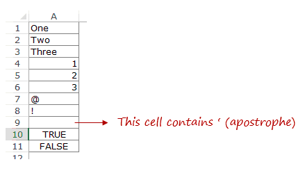
It has all the combinations of text, numbers, blank, special characters, and logical values.

To count cells that contain text values, we will use the wildcard characters:

• Asterisk (*): An asterisk represents any number of characters in excel. For example, ex* could mean excel, excels, example, expert, etc.
• Question Mark (?): A question mark represents one single character. For example, Tr?mp could mean Trump or Tramp.
• Tilde (~): To identify wildcard characters in a string.

See Also: Examples of using Wildcard Characters in Excel.

Now let’s create formulas to count different combinations.

Count Cells that Contain Text in Excel (including Blanks)

Here is the formula:

=COUNTIF(A1:A11,”*”)

This formula uses COUNTIF function with a wildcard character in the criteria. Since asterisk (*) represents any number of characters, it counts all the cells that have text characters in it.

It even counts cells that have an empty string in it (an empty string can be a result of formula returning =”” or a cell that contains an apostrophe). While a cell with empty string looks blank, it is counted by this formula.

Logical Values are not counted.

Count Cells that Contain Text in Excel (excluding Blanks)

Here is the formula:

=COUNTIF(A1:A11,”?*”)

In this formula, the criteria argument is made up of a combination of two wildcard characters (question mark and asterisk). This means that there should, at least, be one character in the cell.

This formula does not count cells that contain an empty string (an apostrophe or =””). Since an empty string has no character in it, it fails the criteria and is not counted.

Logical Values are also not counted.

Count Cells that Contain Text (excluding Blanks, including Logical Values)

Here is the formula:

=COUNTIF(A1:A11,”?*”) + SUMPRODUCT(–(ISLOGICAL(A1:A11))

The first part of the formula uses a combination of wildcard characters (* and ?). This returns the number of cells that have at least one text character in it (counts text and special characters, but does not count cells with empty strings).

The second part of the formula checks for logical values. Excel ISLOGICAL function returns TRUE if there is a logical value and FALSE if there isn’t. A double negative sign ensures that TRUEs are converted into 1 and FALSEs into 0. Excel SUMPRODUCT function then simply returns the number of cells that have a logical value in it.

These above examples demonstrate how to use a combination of formulas and wildcard characters to count cells. In a similar fashion, you can also construct formulas to find the SUM or AVERAGE of a range of cells based on the data type in it.

You May Also Like the Following Excel Tutorials:

• Count the Number of Words in a Text String.
• Using Multiple Criteria in Excel COUNTIF and COUNTIFS Function.
• How to Count Colored Cells in Excel.
• Count Characters in a Cell (or Range of Cells) Using Formulas in Excel