
Excel для Microsoft 365 Excel для Microsoft 365 для Mac Excel для Интернета Excel 2021 Excel 2021 для Mac Excel 2019 Excel 2019 для Mac Excel 2016 Excel 2016 для Mac Excel 2013 Excel 2010 Excel 2007 Excel для Mac 2011 Excel Starter 2010 Еще…Меньше
Функция СЧЁТ подсчитывает количество ячеек, содержащих числа, и количество чисел в списке аргументов. Функция СЧЁТ используется для определения количества числовых ячеек в диапазонах и массивах чисел. Например, для вычисления количества чисел в диапазоне A1:A20 можно ввести следующую формулу: =СЧЁТ(A1:A20). Если в данном примере пять ячеек из диапазона содержат числа, то результатом будет значение 5.

Синтаксис
СЧЁТ(значение1;[значение2];…)
Аргументы функции СЧЁТ указаны ниже.
-
Значение1 — обязательный аргумент. Первый элемент, ссылка на ячейку или диапазон, для которого требуется подсчитать количество чисел.
-
Значение2; … — необязательный аргумент. До 255 дополнительных элементов, ссылок на ячейки или диапазонов, в которых требуется подсчитать количество чисел.
Примечание: Аргументы могут содержать данные различных типов или ссылаться на них, но при подсчете учитываются только числа.
Замечания
-
Учитываются аргументы, являющиеся числами, датами или текстовым представлением чисел (например, число, заключенное в кавычки, такое как «1»).
-
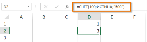
Логические значения и текстовые представления чисел, введенные непосредственно в списке аргументов, также учитываются.
-
Аргументы, являющиеся значениями ошибок или текстом, который нельзя преобразовать в числа, пропускаются.
-
Если аргумент является массивом или ссылкой, то учитываются только числа. Пустые ячейки, логические значения, текст и значения ошибок в массиве или ссылке пропускаются.
-
Если необходимо подсчитать логические значения, элементы текста или значения ошибок, используйте функцию СЧЁТЗ.
-
Если требуется подсчитать только те числа, которые соответствуют определенным критериям, используйте функцию СЧЁТЕСЛИ или СЧЁТЕСЛИМН.
Пример
Скопируйте образец данных из следующей таблицы и вставьте их в ячейку A1 нового листа Excel. Чтобы отобразить результаты формул, выделите их и нажмите клавишу F2, а затем — клавишу ВВОД. При необходимости измените ширину столбцов, чтобы видеть все данные.
|
Данные |
||
|
08.12.2008 |
||
|
19 |
||
|
22,24 |
||
|
ИСТИНА |
||
|
#ДЕЛ/0! |
||
|
Формула |
Описание |
Результат |
|
=СЧЁТ(A2:A7) |
Подсчитывает количество ячеек, содержащих числа, в диапазоне A2:A7. |
3 |
|
=СЧЁТ(A5:A7) |
Подсчитывает количество ячеек, содержащих числа, в диапазоне A5:A7. |
2 |
|
=СЧЁТ(A2:A7;2) |
Подсчитывает количество ячеек, содержащих числа, в диапазоне A2:A7 с учетом числа 2. |
4 |
Нужна дополнительная помощь?
Содержание
- Функция СЧЁТ
- Синтаксис
- Замечания
- Пример
- COUNT function
- Syntax
- Remarks
- Example
- Ways to count values in a worksheet
- Download our examples
- In this article
- Simple counting
- Video: Count cells by using the Excel status bar
- Use AutoSum
- Add a Subtotal row
- Count cells in a list or Excel table column by using the SUBTOTAL function
- Counting based on one or more conditions
- Video: Use the COUNT, COUNTIF, and COUNTA functions
- Count cells in a range by using the COUNT function
- Count cells in a range based on a single condition by using the COUNTIF function
- Count cells in a column based on single or multiple conditions by using the DCOUNT function
- Count cells in a range based on multiple conditions by using the COUNTIFS function
- Count based on criteria by using the COUNT and IF functions together
- Count how often multiple text or number values occur by using the SUM and IF functions together
- Count cells in a column or row in a PivotTable
- Counting when your data contains blank values
- Count nonblank cells in a range by using the COUNTA function
- Count nonblank cells in a list with specific conditions by using the DCOUNTA function
- Count blank cells in a contiguous range by using the COUNTBLANK function
- Count blank cells in a non-contiguous range by using a combination of SUM and IF functions
- Counting unique occurrences of values
- Count the number of unique values in a list column by using Advanced Filter
- Count the number of unique values in a range that meet one or more conditions by using IF, SUM, FREQUENCY, MATCH, and LEN functions
- Special cases (count all cells, count words)
- Count the total number of cells in a range by using ROWS and COLUMNS functions
- Count words in a range by using a combination of SUM, IF, LEN, TRIM, and SUBSTITUTE functions
- Displaying calculations and counts on the status bar
- Need more help?
Функция СЧЁТ
Функция СЧЁТ подсчитывает количество ячеек, содержащих числа, и количество чисел в списке аргументов. Функция СЧЁТ используется для определения количества числовых ячеек в диапазонах и массивах чисел. Например, для вычисления количества чисел в диапазоне A1:A20 можно ввести следующую формулу: =СЧЁТ(A1:A20). Если в данном примере пять ячеек из диапазона содержат числа, то результатом будет значение 5.
Синтаксис
Аргументы функции СЧЁТ указаны ниже.
Значение1 — обязательный аргумент. Первый элемент, ссылка на ячейку или диапазон, для которого требуется подсчитать количество чисел.
Значение2; . — необязательный аргумент. До 255 дополнительных элементов, ссылок на ячейки или диапазонов, в которых требуется подсчитать количество чисел.
Примечание: Аргументы могут содержать данные различных типов или ссылаться на них, но при подсчете учитываются только числа.
Замечания
Учитываются аргументы, являющиеся числами, датами или текстовым представлением чисел (например, число, заключенное в кавычки, такое как «1»).
Логические значения и текстовые представления чисел, введенные непосредственно в списке аргументов, также учитываются.
Аргументы, являющиеся значениями ошибок или текстом, который нельзя преобразовать в числа, пропускаются.
Если аргумент является массивом или ссылкой, то учитываются только числа. Пустые ячейки, логические значения, текст и значения ошибок в массиве или ссылке пропускаются.
Если необходимо подсчитать логические значения, элементы текста или значения ошибок, используйте функцию СЧЁТЗ.
Если требуется подсчитать только те числа, которые соответствуют определенным критериям, используйте функцию СЧЁТЕСЛИ или СЧЁТЕСЛИМН.
Пример
Скопируйте образец данных из следующей таблицы и вставьте их в ячейку A1 нового листа Excel. Чтобы отобразить результаты формул, выделите их и нажмите клавишу F2, а затем — клавишу ВВОД. При необходимости измените ширину столбцов, чтобы видеть все данные.
Источник
COUNT function
The COUNT function counts the number of cells that contain numbers, and counts numbers within the list of arguments. Use the COUNT function to get the number of entries in a number field that is in a range or array of numbers. For example, you can enter the following formula to count the numbers in the range A1:A20: =COUNT(A1:A20). In this example, if five of the cells in the range contain numbers, the result is 5.

Syntax
The COUNT function syntax has the following arguments:
value1 Required. The first item, cell reference, or range within which you want to count numbers.
value2, . Optional. Up to 255 additional items, cell references, or ranges within which you want to count numbers.
Note: The arguments can contain or refer to a variety of different types of data, but only numbers are counted.
Arguments that are numbers, dates, or a text representation of numbers (for example, a number enclosed in quotation marks, such as «1») are counted.
Logical values and text representations of numbers that you type directly into the list of arguments are counted.
Arguments that are error values or text that cannot be translated into numbers are not counted.
If an argument is an array or reference, only numbers in that array or reference are counted. Empty cells, logical values, text, or error values in the array or reference are not counted.
If you want to count logical values, text, or error values, use the COUNTA function.
If you want to count only numbers that meet certain criteria, use the COUNTIF function or the COUNTIFS function.
Example
Copy the example data in the following table, and paste it in cell A1 of a new Excel worksheet. For formulas to show results, select them, press F2, and then press Enter. If you need to, you can adjust the column widths to see all the data.
Источник
Ways to count values in a worksheet
Counting is an integral part of data analysis, whether you are tallying the head count of a department in your organization or the number of units that were sold quarter-by-quarter. Excel provides multiple techniques that you can use to count cells, rows, or columns of data. To help you make the best choice, this article provides a comprehensive summary of methods, a downloadable workbook with interactive examples, and links to related topics for further understanding.
Note: Counting should not be confused with summing. For more information about summing values in cells, columns, or rows, see Summing up ways to add and count Excel data.
Download our examples
You can download an example workbook that gives examples to supplement the information in this article. Most sections in this article will refer to the appropriate worksheet within the example workbook that provides examples and more information.
In this article
Simple counting
You can count the number of values in a range or table by using a simple formula, clicking a button, or by using a worksheet function.
Excel can also display the count of the number of selected cells on the Excel status bar. See the video demo that follows for a quick look at using the status bar. Also, see the section Displaying calculations and counts on the status bar for more information. You can refer to the values shown on the status bar when you want a quick glance at your data and don’t have time to enter formulas.
Video: Count cells by using the Excel status bar
Watch the following video to learn how to view count on the status bar.
Use AutoSum
Use AutoSum by selecting a range of cells that contains at least one numeric value. Then on the Formulas tab, click AutoSum > Count Numbers.

Excel returns the count of the numeric values in the range in a cell adjacent to the range you selected. Generally, this result is displayed in a cell to the right for a horizontal range or in a cell below for a vertical range.
Add a Subtotal row
You can add a subtotal row to your Excel data. Click anywhere inside your data, and then click Data > Subtotal.
Note: The Subtotal option will only work on normal Excel data, and not Excel tables, PivotTables, or PivotCharts.

Also, refer to the following articles:
Count cells in a list or Excel table column by using the SUBTOTAL function
Use the SUBTOTAL function to count the number of values in an Excel table or range of cells. If the table or range contains hidden cells, you can use SUBTOTAL to include or exclude those hidden cells, and this is the biggest difference between SUM and SUBTOTAL functions.
The SUBTOTAL syntax goes like this:

To include hidden values in your range, you should set the function_num argument to 2.
To exclude hidden values in your range, set the function_num argument to 102.
Counting based on one or more conditions
You can count the number of cells in a range that meet conditions (also known as criteria) that you specify by using a number of worksheet functions.
Video: Use the COUNT, COUNTIF, and COUNTA functions
Watch the following video to see how to use the COUNT function and how to use the COUNTIF and COUNTA functions to count only the cells that meet conditions you specify.
Count cells in a range by using the COUNT function
Use the COUNT function in a formula to count the number of numeric values in a range.

In the above example, A2, A3, and A6 are the only cells that contains numeric values in the range, hence the output is 3.
Note: A7 is a time value, but it contains text ( a.m.), hence COUNT does not consider it a numerical value. If you were to remove a.m. from the cell, COUNT will consider A7 as a numerical value, and change the output to 4.
Count cells in a range based on a single condition by using the COUNTIF function
Use the COUNTIF function function to count how many times a particular value appears in a range of cells.

Count cells in a column based on single or multiple conditions by using the DCOUNT function
DCOUNT function counts the cells that contain numbers in a field (column) of records in a list or database that match conditions that you specify.
In the following example, you want to find the count of the months including or later than March 2016 that had more than 400 units sold. The first table in the worksheet, from A1 to B7, contains the sales data.

DCOUNT uses conditions to determine where the values should be returned from. Conditions are typically entered in cells in the worksheet itself, and you then refer to these cells in the criteria argument. In this example, cells A10 and B10 contain two conditions—one that specifies that the return value must be greater than 400, and the other that specifies that the ending month should be equal to or greater than March 31st, 2016.
You should use the following syntax:
DCOUNT checks the data in the range A1 through B7, applies the conditions specified in A10 and B10, and returns 2, the total number of rows that satisfy both conditions (rows 5 and 7).
Count cells in a range based on multiple conditions by using the COUNTIFS function
The COUNTIFS function is similar to the COUNTIF function with one important exception: COUNTIFS lets you apply criteria to cells across multiple ranges and counts the number of times all criteria are met. You can use up to 127 range/criteria pairs with COUNTIFS.
The syntax for COUNTIFS is:
COUNTIFS(criteria_range1, criteria1, [criteria_range2, criteria2],…)
See the following example:

Count based on criteria by using the COUNT and IF functions together
Let’s say you need to determine how many salespeople sold a particular item in a certain region or you want to know how many sales over a certain value were made by a particular salesperson. You can use the IF and COUNT functions together; that is, you first use the IF function to test a condition and then, only if the result of the IF function is True, you use the COUNT function to count cells.
The formulas in this example must be entered as array formulas. If you have opened this workbook in Excel for Windows or Excel 2016 for Mac and want to change the formula or create a similar formula, press F2, and then press Ctrl+Shift+Enter to make the formula return the results you expect. In earlier versions of Excel for Mac, use  +Shift+Enter.
For the example formulas to work, the second argument for the IF function must be a number.

Count how often multiple text or number values occur by using the SUM and IF functions together
In the examples that follow, we use the IF and SUM functions together. The IF function first tests the values in some cells and then, if the result of the test is True, SUM totals those values that pass the test.

The above function says if C2:C7 contains the values Buchanan and Dodsworth, then the SUM function should display the sum of records where the condition is met. The formula finds three records for Buchanan and one for Dodsworth in the given range, and displays 4.

The above function says if D2:D7 contains values lesser than $9000 or greater than $19,000, then SUM should display the sum of all those records where the condition is met. The formula finds two records D3 and D5 with values lesser than $9000, and then D4 and D6 with values greater than $19,000, and displays 4.

The above function says if D2:D7 has invoices for Buchanan for less than $9000, then SUM should display the sum of records where the condition is met. The formula finds that C6 meets the condition, and displays 1.
Important: The formulas in this example must be entered as array formulas. That means you press F2 and then press Ctrl+Shift+Enter. In earlier versions of Excel for Mac use +Shift+Enter.
See the following Knowledge Base articles for additional tips:
Count cells in a column or row in a PivotTable
A PivotTable summarizes your data and helps you analyze and drill down into your data by letting you choose the categories on which you want to view your data.
You can quickly create a PivotTable by selecting a cell in a range of data or Excel table and then, on the Insert tab, in the Tables group, clicking PivotTable.

Let’s look at a sample scenario of a Sales spreadsheet, where you can count how many sales values are there for Golf and Tennis for specific quarters.
Note: For an interactive experience, you can run these steps on the sample data provided in the PivotTable sheet in the downloadable workbook.
Enter the following data in an Excel spreadsheet.

Click Insert > PivotTable.
In the Create PivotTable dialog box, click Select a table or range, then click New Worksheet, and then click OK.
An empty PivotTable is created in a new sheet.
In the PivotTable Fields pane, do the following:
Drag Sport to the Rows area.
Drag Quarter to the Columns area.
Drag Sales to the Values area.
The field name displays as SumofSales2 in both the PivotTable and the Values area.
At this point, the PivotTable Fields pane looks like this:

In the Values area, click the dropdown next to SumofSales2 and select Value Field Settings.
In the Value Field Settings dialog box, do the following:
In the Summarize value field by section, select Count.
In the Custom Name field, modify the name to Count.

The PivotTable displays the count of records for Golf and Tennis in Quarter 3 and Quarter 4, along with the sales figures.

Counting when your data contains blank values
You can count cells that either contain data or are blank by using worksheet functions.
Count nonblank cells in a range by using the COUNTA function
Use the COUNTA function function to count only cells in a range that contain values.
When you count cells, sometimes you want to ignore any blank cells because only cells with values are meaningful to you. For example, you want to count the total number of salespeople who made a sale (column D).

COUNTA ignores the blank values in D3, D4, D8, and D11, and counts only the cells containing values in column D. The function finds six cells in column D containing values and displays 6 as the output.
Count nonblank cells in a list with specific conditions by using the DCOUNTA function
Use the DCOUNTA function to count nonblank cells in a column of records in a list or database that match conditions that you specify.
The following example uses the DCOUNTA function to count the number of records in the database that is contained in the range A1:B7 that meet the conditions specified in the criteria range A9:B10. Those conditions are that the Product ID value must be greater than or equal to 2000 and the Ratings value must be greater than or equal to 50.

DCOUNTA finds two rows that meet the conditions- rows 2 and 4, and displays the value 2 as the output.
Count blank cells in a contiguous range by using the COUNTBLANK function
Use the COUNTBLANK function function to return the number of blank cells in a contiguous range (cells are contiguous if they are all connected in an unbroken sequence). If a cell contains a formula that returns empty text («»), that cell is counted.
When you count cells, there may be times when you want to include blank cells because they are meaningful to you. In the following example of a grocery sales spreadsheet. suppose you want to find out how many cells don’t have the sales figures mentioned.

Note: The COUNTBLANK worksheet function provides the most convenient method for determining the number of blank cells in a range, but it doesn’t work very well when the cells of interest are in a closed workbook or when they do not form a contiguous range. The Knowledge Base article XL: When to Use SUM(IF()) instead of CountBlank() shows you how to use a SUM(IF()) array formula in those cases.
Count blank cells in a non-contiguous range by using a combination of SUM and IF functions
Use a combination of the SUM function and the IF function. In general, you do this by using the IF function in an array formula to determine whether each referenced cell contains a value, and then summing the number of FALSE values returned by the formula.
See a few examples of SUM and IF function combinations in an earlier section Count how often multiple text or number values occur by using the SUM and IF functions together in this topic.
Counting unique occurrences of values
You can count unique values in a range by using a PivotTable, COUNTIF function, SUM and IF functions together, or the Advanced Filter dialog box.
Count the number of unique values in a list column by using Advanced Filter
Use the Advanced Filter dialog box to find the unique values in a column of data. You can either filter the values in place or you can extract and paste them to a new location. Then you can use the ROWS function to count the number of items in the new range.
To use Advanced Filter, click the Data tab, and in the Sort & Filter group, click Advanced.
The following figure shows how you use the Advanced Filter to copy only the unique records to a new location on the worksheet.

In the following figure, column E contains the values that were copied from the range in column D.

If you filter your data in place, values are not deleted from your worksheet — one or more rows might be hidden. Click Clear in the Sort & Filter group on the Data tab to display those values again.
If you only want to see the number of unique values at a quick glance, select the data after you have used the Advanced Filter (either the filtered or the copied data) and then look at the status bar. The Count value on the status bar should equal the number of unique values.
Count the number of unique values in a range that meet one or more conditions by using IF, SUM, FREQUENCY, MATCH, and LEN functions
Use various combinations of the IF, SUM, FREQUENCY, MATCH, and LEN functions.
For more information and examples, see the section «Count the number of unique values by using functions» in the article Count unique values among duplicates.
Special cases (count all cells, count words)
You can count the number of cells or the number of words in a range by using various combinations of worksheet functions.
Count the total number of cells in a range by using ROWS and COLUMNS functions
Suppose you want to determine the size of a large worksheet to decide whether to use manual or automatic calculation in your workbook. To count all the cells in a range, use a formula that multiplies the return values using the ROWS and COLUMNS functions. See the following image for an example:

Count words in a range by using a combination of SUM, IF, LEN, TRIM, and SUBSTITUTE functions
You can use a combination of the SUM, IF, LEN, TRIM, and SUBSTITUTE functions in an array formula. The following example shows the result of using a nested formula to find the number of words in a range of 7 cells (3 of which are empty). Some of the cells contain leading or trailing spaces — the TRIM and SUBSTITUTE functions remove these extra spaces before any counting occurs. See the following example:

Now, for the above formula to work correctly, you have to make this an array formula, otherwise the formula returns the #VALUE! error. To do that, click on the cell that has the formula, and then in the Formula bar, press Ctrl + Shift + Enter. Excel adds a curly bracket at the beginning and the end of the formula, thus making it an array formula.
For more information on array formulas, see Overview of formulas in Excel and Create an array formula.
Displaying calculations and counts on the status bar
When one or more cells are selected, information about the data in those cells is displayed on the Excel status bar. For example, if four cells on your worksheet are selected, and they contain the values 2, 3, a text string (such as «cloud»), and 4, all of the following values can be displayed on the status bar at the same time: Average, Count, Numerical Count, Min, Max, and Sum. Right-click the status bar to show or hide any or all of these values. These values are shown in the illustration that follows.

Need more help?
You can always ask an expert in the Excel Tech Community or get support in the Answers community.
Источник
На чтение 1 мин
Функция СЧЁТ (COUNT) в Excel используется для подсчета ячеек с числовыми значениями.
Содержание
- Что возвращает функция
- Синтаксис
- Аргументы функции
- Дополнительная информация
- Примеры использования функции СЧЕТ в Excel
Что возвращает функция
Возвращает значение количества ячеек с числами.
 Больше лайфхаков в нашем Telegram Подписаться
Синтаксис
=COUNT(value1, [value2], …) — английская версия
=СЧЁТ(значение1;[значение2];…) — русская версия
Аргументы функции
- value1 (значение1) — ссылка на ячейку или диапазон, в котором вы хотите посчитать количество чисел;
- [value2],…([значение2]) — (необязательный аргумент) до 255 дополнительных ячеек со значениями, по которым вы хотите посчитать количество чисел.
Дополнительная информация
- Функция считает только ячейки с числовыми значениями (1,2,3…и.т.д.);
- Значения даты или текст в виде чисел в кавычках (например единица в кавычках — «1») учитываются функцией;
- Логические значения в ячейках не подсчитываются;
- Ячейки с ошибками и текстом не участвуют в подсчете;
- Пустые ячейки, логические значения, текст или ячейки с ошибками в массиве или ссылке не учитываются.
Примеры использования функции СЧЕТ в Excel
На чтение 2 мин Опубликовано 11.01.2015
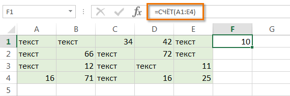
Функция СЧЕТ в Excel подсчитывает количество числовых значений в списке аргументов. Самым традиционным способом применения данной функции является подсчет количества ячеек в Excel, содержащих числа. К примеру, следующая формула возвращает количество ячеек в диапазоне A1:E4, которые содержат числа.
Содержание
- Синтаксис функции СЧЕТ
- Какие значения считаются числовыми
- Полезная информация
- Примеры использования функции СЧЕТ в Excel
Синтаксис функции СЧЕТ
СЧЕТ(значение1; [значение2]; …)
COUNT(value1, [value2], …)
В качестве аргументов функции СЧЕТ могут выступать любые значения, ссылки на ячейки и диапазоны, массивы данных, а также формулы и функции.
Значение1 (value1) – обязательный аргумент функции СЧЕТ, все остальные аргументы являются необязательными и могут быть опущены.
Начиная с версии Excel 2007, Вы можете использовать до 255 аргументов, каждый из которых способен содержать огромное количество данных. В более ранних версиях Excel (например, Excel 2003 года), функция СЧЕТ обрабатывала лишь 30 аргументов.
Какие значения считаются числовыми
В Microsoft Excel аргументы функции СЧЕТ могут содержать самые различные данные, либо ссылаться на них. При этом важно понимать какие значения функция СЧЕТ принимает за числовые, а какие просто игнорирует.
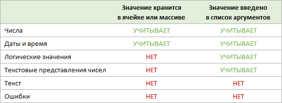
- Числа, даты и время всегда учитываются функцией СЧЕТ как числовые.
- Пустые ячейки, ошибки и текст, который не может быть преобразован в числа, функция СЧЕТ игнорирует.
- Логические значения, а также текстовые представления чисел (например, число, заключенное в кавычки), учитываются функцией СЧЕТ по-разному. Все зависит от того, где хранится значение: в ячейке, массиве или введено непосредственно в список аргументов.
В таблице ниже представлено, какие значения функция СЧЕТ учитывает, как числовые, а какие нет.
Полезная информация
- Чтобы посчитать количество непустых ячеек в диапазоне, воспользуйтесь функцией СЧЕТЗ.
- Если требуется посчитать количество пустых ячеек в Excel, используйте функцию СЧИТАТЬПУСТОТЫ.
- Для подсчета количества ячеек по условию Вы можете применить функции СЧЕТЕСЛИ и СЧЕТЕСЛИМН.
Примеры использования функции СЧЕТ в Excel
- Следующая формула подсчитывает количество ячеек, содержащих числовые значения. Подсчет ведется сразу по двум диапазонам. Красным выделены ячейки, которые учитываются функцией СЧЕТ.

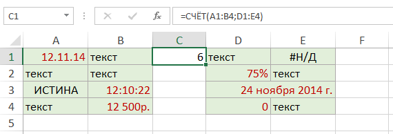
- Данная формула подсчитывает количество чисел в массиве данных, который состоит из трех значений. Логическое значение и текстовое представление числа функция СЧЕТ не учла.
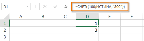
- Если эти же три значения подставить прямо на место аргументов функции, то все они будут учтены, и результат окажется другим.
Оцените качество статьи. Нам важно ваше мнение:
Usage notes
The COUNT function returns the count of numeric values in the list of supplied arguments. COUNT takes multiple arguments in the form value1, value2, value3, etc. Arguments can be individual hardcoded values, cell references, or ranges up to a total of 255 arguments. All numbers are counted, including negative numbers, percentages, dates, times, fractions, and formulas that return numbers. Empty cells and text values are ignored.
Examples
The COUNT function counts numeric values and ignores text values:
=COUNT(1,2,3) // returns 3
=COUNT(1,"a","b") // returns 1
=COUNT("apple",100,125,150,"orange") // returns 3
Typically, the COUNT function is used on a range. For example, to count numeric values in the range A1:A10:
=COUNT(A1:A100) // count numbers in A1:A10
In the example shown, COUNT is set up to count numbers in the range B5:B15:
=COUNT(B5:B15) // returns 6
COUNT returns 6, since there are 6 numeric values in the range B5:B15. Text values and blank cells are ignored. Note that dates and times are numbers, and therefore included in the count.
The COUNTA function works like the COUNT function, but COUNTA includes numbers and text in the count.
Functions for counting
- To count numbers only, use the COUNT function.
- To count numbers and text, use the COUNTA function.
- To count with one condition, use the COUNTIF function
- To count with multiple conditions, use the COUNTIFS function.
- To count empty cells, use the COUNTBLANK function.
Notes
- COUNT can handle up to 255 arguments.
- COUNT ignores the logical values TRUE and FALSE.
- COUNT ignores text values and empty cells.