
Counting is an integral part of data analysis, whether you are tallying the head count of a department in your organization or the number of units that were sold quarter-by-quarter. Excel provides multiple techniques that you can use to count cells, rows, or columns of data. To help you make the best choice, this article provides a comprehensive summary of methods, a downloadable workbook with interactive examples, and links to related topics for further understanding.
Download our examples
You can download an example workbook that gives examples to supplement the information in this article. Most sections in this article will refer to the appropriate worksheet within the example workbook that provides examples and more information.
Download examples to count values in a spreadsheet
In this article
-
Simple counting
-
Use AutoSum
-
Add a Subtotal row
-
Count cells in a list or Excel table column by using the SUBTOTAL function
-
-
Counting based on one or more conditions
-
Video: Use the COUNT, COUNTIF, and COUNTA functions
-
Count cells in a range by using the COUNT function
-
Count cells in a range based on a single condition by using the COUNTIF function
-
Count cells in a column based on single or multiple conditions by using the DCOUNT function
-
Count cells in a range based on multiple conditions by using the COUNTIFS function
-
Count based on criteria by using the COUNT and IF functions together
-
Count how often multiple text or number values occur by using the SUM and IF functions together
-
Count cells in a column or row in a PivotTable
-
-
Counting when your data contains blank values
-
Count nonblank cells in a range by using the COUNTA function
-
Count nonblank cells in a list with specific conditions by using the DCOUNTA function
-
Count blank cells in a contiguous range by using the COUNTBLANK function
-
Count blank cells in a non-contiguous range by using a combination of SUM and IF functions
-
-
Counting unique occurrences of values
-
Count the number of unique values in a list column by using Advanced Filter
-
Count the number of unique values in a range that meet one or more conditions by using IF, SUM, FREQUENCY, MATCH, and LEN functions
-
-
Special cases (count all cells, count words)
-
Count the total number of cells in a range by using ROWS and COLUMNS functions
-
Count words in a range by using a combination of SUM, IF, LEN, TRIM, and SUBSTITUTE functions
-
-
Displaying calculations and counts on the status bar
Simple counting
You can count the number of values in a range or table by using a simple formula, clicking a button, or by using a worksheet function.
Excel can also display the count of the number of selected cells on the Excel status bar. See the video demo that follows for a quick look at using the status bar. Also, see the section Displaying calculations and counts on the status bar for more information. You can refer to the values shown on the status bar when you want a quick glance at your data and don’t have time to enter formulas.
Video: Count cells by using the Excel status bar
Watch the following video to learn how to view count on the status bar.

Use AutoSum
Use AutoSum by selecting a range of cells that contains at least one numeric value. Then on the Formulas tab, click AutoSum > Count Numbers.

Excel returns the count of the numeric values in the range in a cell adjacent to the range you selected. Generally, this result is displayed in a cell to the right for a horizontal range or in a cell below for a vertical range.
Top of Page
Add a Subtotal row
You can add a subtotal row to your Excel data. Click anywhere inside your data, and then click Data > Subtotal.
Note: The Subtotal option will only work on normal Excel data, and not Excel tables, PivotTables, or PivotCharts.

Also, refer to the following articles:
-
Outline (group) data in a worksheet
-
Insert subtotals in a list of data in a worksheet
Top of Page
Count cells in a list or Excel table column by using the SUBTOTAL function
Use the SUBTOTAL function to count the number of values in an Excel table or range of cells. If the table or range contains hidden cells, you can use SUBTOTAL to include or exclude those hidden cells, and this is the biggest difference between SUM and SUBTOTAL functions.
The SUBTOTAL syntax goes like this:
SUBTOTAL(function_num,ref1,[ref2],…)

To include hidden values in your range, you should set the function_num argument to 2.
To exclude hidden values in your range, set the function_num argument to 102.
Top of Page
Counting based on one or more conditions
You can count the number of cells in a range that meet conditions (also known as criteria) that you specify by using a number of worksheet functions.
Video: Use the COUNT, COUNTIF, and COUNTA functions
Watch the following video to see how to use the COUNT function and how to use the COUNTIF and COUNTA functions to count only the cells that meet conditions you specify.
Top of Page
Count cells in a range by using the COUNT function
Use the COUNT function in a formula to count the number of numeric values in a range.

In the above example, A2, A3, and A6 are the only cells that contains numeric values in the range, hence the output is 3.
Note: A7 is a time value, but it contains text (a.m.), hence COUNT does not consider it a numerical value. If you were to remove a.m. from the cell, COUNT will consider A7 as a numerical value, and change the output to 4.
Top of Page
Count cells in a range based on a single condition by using the COUNTIF function
Use the COUNTIF function function to count how many times a particular value appears in a range of cells.

Top of Page
Count cells in a column based on single or multiple conditions by using the DCOUNT function
DCOUNT function counts the cells that contain numbers in a field (column) of records in a list or database that match conditions that you specify.
In the following example, you want to find the count of the months including or later than March 2016 that had more than 400 units sold. The first table in the worksheet, from A1 to B7, contains the sales data.

DCOUNT uses conditions to determine where the values should be returned from. Conditions are typically entered in cells in the worksheet itself, and you then refer to these cells in the criteria argument. In this example, cells A10 and B10 contain two conditions—one that specifies that the return value must be greater than 400, and the other that specifies that the ending month should be equal to or greater than March 31st, 2016.
You should use the following syntax:
=DCOUNT(A1:B7,»Month ending»,A9:B10)
DCOUNT checks the data in the range A1 through B7, applies the conditions specified in A10 and B10, and returns 2, the total number of rows that satisfy both conditions (rows 5 and 7).
Top of Page
Count cells in a range based on multiple conditions by using the COUNTIFS function
The COUNTIFS function is similar to the COUNTIF function with one important exception: COUNTIFS lets you apply criteria to cells across multiple ranges and counts the number of times all criteria are met. You can use up to 127 range/criteria pairs with COUNTIFS.
The syntax for COUNTIFS is:
COUNTIFS(criteria_range1, criteria1, [criteria_range2, criteria2],…)
See the following example:

Top of Page
Count based on criteria by using the COUNT and IF functions together
Let’s say you need to determine how many salespeople sold a particular item in a certain region or you want to know how many sales over a certain value were made by a particular salesperson. You can use the IF and COUNT functions together; that is, you first use the IF function to test a condition and then, only if the result of the IF function is True, you use the COUNT function to count cells.
Notes:
-
The formulas in this example must be entered as array formulas. If you have opened this workbook in Excel for Windows or Excel 2016 for Mac and want to change the formula or create a similar formula, press F2, and then press Ctrl+Shift+Enter to make the formula return the results you expect. In earlier versions of Excel for Mac, use
 +Shift+Enter.
 -
For the example formulas to work, the second argument for the IF function must be a number.

Top of Page
Count how often multiple text or number values occur by using the SUM and IF functions together
In the examples that follow, we use the IF and SUM functions together. The IF function first tests the values in some cells and then, if the result of the test is True, SUM totals those values that pass the test.
Example 1

The above function says if C2:C7 contains the values Buchanan and Dodsworth, then the SUM function should display the sum of records where the condition is met. The formula finds three records for Buchanan and one for Dodsworth in the given range, and displays 4.
Example 2

The above function says if D2:D7 contains values lesser than $9000 or greater than $19,000, then SUM should display the sum of all those records where the condition is met. The formula finds two records D3 and D5 with values lesser than $9000, and then D4 and D6 with values greater than $19,000, and displays 4.
Example 3

The above function says if D2:D7 has invoices for Buchanan for less than $9000, then SUM should display the sum of records where the condition is met. The formula finds that C6 meets the condition, and displays 1.
Important: The formulas in this example must be entered as array formulas. That means you press F2 and then press Ctrl+Shift+Enter. In earlier versions of Excel for Mac use  +Shift+Enter.
See the following Knowledge Base articles for additional tips:
-
XL: Using SUM(IF()) As an Array Function Instead of COUNTIF() with AND
-
XL: How to Count the Occurrences of a Number or Text in a Range
Top of Page
Count cells in a column or row in a PivotTable
A PivotTable summarizes your data and helps you analyze and drill down into your data by letting you choose the categories on which you want to view your data.
You can quickly create a PivotTable by selecting a cell in a range of data or Excel table and then, on the Insert tab, in the Tables group, clicking PivotTable.

Let’s look at a sample scenario of a Sales spreadsheet, where you can count how many sales values are there for Golf and Tennis for specific quarters.
Note: For an interactive experience, you can run these steps on the sample data provided in the PivotTable sheet in the downloadable workbook.
-
Enter the following data in an Excel spreadsheet.
-
Select A2:C8
-
Click Insert > PivotTable.
-
In the Create PivotTable dialog box, click Select a table or range, then click New Worksheet, and then click OK.
An empty PivotTable is created in a new sheet.
-
In the PivotTable Fields pane, do the following:
-
Drag Sport to the Rows area.
-
Drag Quarter to the Columns area.
-
Drag Sales to the Values area.
-
Repeat step c.
The field name displays as SumofSales2 in both the PivotTable and the Values area.
At this point, the PivotTable Fields pane looks like this:
-
In the Values area, click the dropdown next to SumofSales2 and select Value Field Settings.
-
In the Value Field Settings dialog box, do the following:
-
In the Summarize value field by section, select Count.
-
In the Custom Name field, modify the name to Count.
-
Click OK.
-
The PivotTable displays the count of records for Golf and Tennis in Quarter 3 and Quarter 4, along with the sales figures.
-


Top of Page
Counting when your data contains blank values
You can count cells that either contain data or are blank by using worksheet functions.
Count nonblank cells in a range by using the COUNTA function
Use the COUNTA function function to count only cells in a range that contain values.
When you count cells, sometimes you want to ignore any blank cells because only cells with values are meaningful to you. For example, you want to count the total number of salespeople who made a sale (column D).

COUNTA ignores the blank values in D3, D4, D8, and D11, and counts only the cells containing values in column D. The function finds six cells in column D containing values and displays 6 as the output.
Top of Page
Count nonblank cells in a list with specific conditions by using the DCOUNTA function
Use the DCOUNTA function to count nonblank cells in a column of records in a list or database that match conditions that you specify.
The following example uses the DCOUNTA function to count the number of records in the database that is contained in the range A1:B7 that meet the conditions specified in the criteria range A9:B10. Those conditions are that the Product ID value must be greater than or equal to 2000 and the Ratings value must be greater than or equal to 50.

DCOUNTA finds two rows that meet the conditions- rows 2 and 4, and displays the value 2 as the output.
Top of Page
Count blank cells in a contiguous range by using the COUNTBLANK function
Use the COUNTBLANK function function to return the number of blank cells in a contiguous range (cells are contiguous if they are all connected in an unbroken sequence). If a cell contains a formula that returns empty text («»), that cell is counted.
When you count cells, there may be times when you want to include blank cells because they are meaningful to you. In the following example of a grocery sales spreadsheet. suppose you want to find out how many cells don’t have the sales figures mentioned.

Note: The COUNTBLANK worksheet function provides the most convenient method for determining the number of blank cells in a range, but it doesn’t work very well when the cells of interest are in a closed workbook or when they do not form a contiguous range. The Knowledge Base article XL: When to Use SUM(IF()) instead of CountBlank() shows you how to use a SUM(IF()) array formula in those cases.
Top of Page
Count blank cells in a non-contiguous range by using a combination of SUM and IF functions
Use a combination of the SUM function and the IF function. In general, you do this by using the IF function in an array formula to determine whether each referenced cell contains a value, and then summing the number of FALSE values returned by the formula.
See a few examples of SUM and IF function combinations in an earlier section Count how often multiple text or number values occur by using the SUM and IF functions together in this topic.
Top of Page
Counting unique occurrences of values
You can count unique values in a range by using a PivotTable, COUNTIF function, SUM and IF functions together, or the Advanced Filter dialog box.
Count the number of unique values in a list column by using Advanced Filter
Use the Advanced Filter dialog box to find the unique values in a column of data. You can either filter the values in place or you can extract and paste them to a new location. Then you can use the ROWS function to count the number of items in the new range.
To use Advanced Filter, click the Data tab, and in the Sort & Filter group, click Advanced.
The following figure shows how you use the Advanced Filter to copy only the unique records to a new location on the worksheet.

In the following figure, column E contains the values that were copied from the range in column D.

Notes:
-
If you filter your data in place, values are not deleted from your worksheet — one or more rows might be hidden. Click Clear in the Sort & Filter group on the Data tab to display those values again.
-
If you only want to see the number of unique values at a quick glance, select the data after you have used the Advanced Filter (either the filtered or the copied data) and then look at the status bar. The Count value on the status bar should equal the number of unique values.
For more information, see Filter by using advanced criteria
Top of Page
Count the number of unique values in a range that meet one or more conditions by using IF, SUM, FREQUENCY, MATCH, and LEN functions
Use various combinations of the IF, SUM, FREQUENCY, MATCH, and LEN functions.
For more information and examples, see the section «Count the number of unique values by using functions» in the article Count unique values among duplicates.
Top of Page
Special cases (count all cells, count words)
You can count the number of cells or the number of words in a range by using various combinations of worksheet functions.
Count the total number of cells in a range by using ROWS and COLUMNS functions
Suppose you want to determine the size of a large worksheet to decide whether to use manual or automatic calculation in your workbook. To count all the cells in a range, use a formula that multiplies the return values using the ROWS and COLUMNS functions. See the following image for an example:

Top of Page
Count words in a range by using a combination of SUM, IF, LEN, TRIM, and SUBSTITUTE functions
You can use a combination of the SUM, IF, LEN, TRIM, and SUBSTITUTE functions in an array formula. The following example shows the result of using a nested formula to find the number of words in a range of 7 cells (3 of which are empty). Some of the cells contain leading or trailing spaces — the TRIM and SUBSTITUTE functions remove these extra spaces before any counting occurs. See the following example:

Now, for the above formula to work correctly, you have to make this an array formula, otherwise the formula returns the #VALUE! error. To do that, click on the cell that has the formula, and then in the Formula bar, press Ctrl + Shift + Enter. Excel adds a curly bracket at the beginning and the end of the formula, thus making it an array formula.
For more information on array formulas, see Overview of formulas in Excel and Create an array formula.
Top of Page
Displaying calculations and counts on the status bar
When one or more cells are selected, information about the data in those cells is displayed on the Excel status bar. For example, if four cells on your worksheet are selected, and they contain the values 2, 3, a text string (such as «cloud»), and 4, all of the following values can be displayed on the status bar at the same time: Average, Count, Numerical Count, Min, Max, and Sum. Right-click the status bar to show or hide any or all of these values. These values are shown in the illustration that follows.

Top of Page
Need more help?
You can always ask an expert in the Excel Tech Community or get support in the Answers community.
Data analysis usually involves large data sets, and at some point, one may need to find out the number of values that appear only once in the dataset. In this case, you will be counting without duplicates. Unique values are values that appear only once in a dataset.
If you are faced with mountains of data, then counting without duplicates might be very arduous. More so, Excel does not have a special formula for counting without duplicates. However, there is always a way out! This tutorial will serve as a guide on how to count unique and distinct values without duplicating them.

Take a look at the numbers in the table above; the unique values are not duplicated. They don’t appear more than once. Whereas, distinct values are the different numbers in the collection. In the table below, we have separated the unique values from distinct values.

1. Using the array COUNTIF formula
The COUNTIF function counts the frequency of occurrence of each value within the range. To get the number of the unique values, you have to sum them up. You can do this efficiently by combining SUM and COUNTIF functions. A combo of two functions can count unique values without duplication.
Below is the syntax:
=SUM(IF(COUNTIF(data, data)=1,1,0)).
The formula contains three separate functions – SUM, IF, and COUNTIF.
COUNTIF function» counts how many times a particular number appears within the range.
«IF function» analysis the results returned by the «COUNTIF» function. It maintains the 1’s for unique values and replaces other values with «0.»
Note: Always press Ctrl + Shift + Enter when entering your array formula.

CTRL+SHIFT+ENTER allow excel to recognize the formula as an array function. unique value= =SUM(IF(COUNTIF(A2:A10, A2:A10)=1,1,0))
Alternatively, you can use the SUMPRODUCT formula to avoid the use of CTRL+SHIFT+ENTER.
Below is the syntax:
=SUMPRODUCT(1/COUNTIF(range, criteria)).
In the example below, we have a list of items with duplicates.

If we use the SUM formula to count the total number of items, there will be duplicates. To exclude the duplicates, you have to follow these steps.
Step 1: Go to cell D1 and enter this formula “=SUMPRODUCT(1/COUNTIF( B1:B11,B1:B11)). B1:B11 is the array range you want to count the total number of unique values in the list.

Step 2: Press enter and the results will be displayed in cell D1. From the displayed results (6) we can see there are no duplicates.

The above formula counts the values of the six items A/B/C/D/E/F.
2. Using a combination of SUM, IF, FREQUENCY, MATCH, and ROW Function
If we want to count unique values that exclude all duplicates (that appear in more than one product), use the combination of these functions.
- The sum function allows you to add the values.
- For each true condition of IF function, assign value 1.
- The FREQUENCY function allows you to count the number of values ignoring texts and zeros. In the first occurrence of the distinct value, it returns an equal number to the number of occurrences of that value. It returns zero for the occurrences that have the same value after the first occurrence.
- The MATCH function returns the position of the text value in an array range. The return value acts as the function argument for FREQUENCY.
- The ROW function returns the row reference number.
Example: Enter the following formula to count unique values by excluding all duplicates
=SUM(IF(FREQUENCY(MATCH(B1:B11,B1:B11,0),ROW(B1:B11)-ROW(B1)+1)=1,1))

Press enter. The unique value is 3 (Item D/E/F).

3. Using ISNUMBER Function to count numeric numbers
The function we used earlier counts, both texts and numbers, without duplicating. To count only numerals without duplicating, you have to include ISNUMBER function in the formula for finding unique values.
=SUM(IF(ISNUMBER(A2:A10)*COUNTIF(A2:A10,A2:A10)=1,1,0))
Note: Always press Ctrl + Shift + Enter when entering your array formula.
Meanwhile, the lowdown in this function is that it also counts dates and times.

4. Using ISTEXT Function to count text values
You can count the number of texts without duplicating by including the ISTEXT function in the array formula as stated below:
=SUM(IF(ISTEXT(A2:A10)*COUNTIF(A2:A10,A2:A10)=1,1,0))
This formula will display the number of unique texts. It excludes errors, blank cells, logical numbers, numbers, etc.
Always press Ctrl + Shift + Enter when entering your array formula.

5. Using Pivot Table to count text values
Easies way to count the value is by creating the pivot table and using the Count of items
1. Create a pivot table

2. Use Count of Items

3. Output Table

6. Using A Filter
The Filter method is the simplest approach that allows you to remove duplicates and remain with unique values. You can, therefore, use two tricks to get unique values as discussed below.
6.1: Filtering for Unique Values
Steps:
1. Select and make sure the range of cells you want to make unique is in a table.
2. Click on Data then select the Advanced option in the soft & filter group.

3. When the Advanced Filter box pops up, you can filter the range of cells or tables by clicking on the Filer the List, in-place option.

4. You can also copy the result of the filter to another location by clicking on the Copy to another location option.
5. Enter a cell reference in the Copy To box.

6. Alternatively, you can click the Collapse Dialog option to hide the popup window temporarily, select a cell on the worksheet, and then click the Expand option.
7. Finish by checking the Unique Records Only and click OK.

6.2: Removing The Duplicates
The method only affects the values in the range of cells or tables and not values outside. After removing the duplicates, you will keep the first occurrence of the value in the list, while the identical values will be deleted. Therefore, remember to copy the original range of cells to the table to another worksheet before deleting duplicates.
Steps:
1. Start by selecting the active range of cells in a table.
2. Select the Data Tab and click Remove Duplicates in the Data Tools group.
3. You can select one or more columns under the Columns face. Alternatively, you can click Select All to select all columns quickly or Unselect All to clear all columns quickly.
4. Click OK and a message will pop up showing how many duplicates you have removed or how many unique values remain. To dismiss the message, click OK.
5. You can undo the change by clicking Undo or pressing Ctrl + Z
7. Using Amazing Excel Tools
Another simple way to count without duplicates in excel is tools like Kutools by the following steps.
1. Select a blank cell to output the result.
2. Click Kutools>Formula>Helper>Formula Helper.
3. Do the following steps in the formula helper dialog;
- Check and select Count unique values in the Choose a formula box. You can check the filter box and type some words to filter the formula names.
- Then choose the range in which you want to count unique values in the range box.
- Press the OK button.
8. Using A Data Model with A Pivot Table to Count Unique Values
The method applies to newer versions of Microsoft Excel, including Microsoft 365, Excel 2019, Excel 2016, and Excel 2013. To count unique values using this approach, follow these steps:
1. Select any cell in the data and click on the Insert tab in the ribbon.
2. Click on Pivot Table to open a dialogue box.
3. Select the Add this data to the Data Model at the bottom and click OK.
4. In the resulting window, drag the Name column into the Name field and the Profession column or any other in the dataset into the Values field.

5. Click on the small arrow next to the Count of Profession option in the Pivot Table fields.
6. Select the Value Field Settings at the bottom.

7. Finish by selecting the Distinct Count or Unique Count option and click OK.

8. You will have your unique values in the Pivot Table.

9. Using Power Pivot
Power Pivot is also another powerful method you can use to count unique values. However, you will need an enabled Power Pivot tab in your ribbon. That means if your Excel version does not have an already-enabled Power Pivot add-in, you will have to enable it first. Once you have enabled it, you can proceed with the following steps:
1. Go to the Data Model and select the Manage Button.

2. This will open a new blank window if it is your first time importing data.
3. Click on Home Tab and select the “Get External Data” option.

4. You will see various sources and options to upload data. Since you want to upload simple Excel, select the «From Other Sources» option.
5. Scroll down to the end of a new dialogue box opened, select “Excel File”, and click Next.

6. You will need to rename the connection created. For simplicity, you can rename it “Excel”. After that, click on “Browse” to choose an Excel file path.
7. You can click on the “Use the first row as column header” option to make the top column the header. Click on the Next Button to finish.

8. You will see the file imported to the Data Model. Click the Finish button.

9. After importing all the rows successfully, hit the Close Button.

10. With your new worksheet, you will have to create a Pivot Table by clicking on Home and then Pivot Table.

11. Click on the small triangle next to it to expand the columns. That is because you already have the data on the first sheet.

12. After dragging and dropping all the data in their respective fields, you will get a simple Pivot Table.

13. Go back to the Power Pivot window and select the Measure option to create a New Measure.

14. Add your desired description name by typing in the box and the suggestions will pop up automatically. Since you want to count unique values, select the Unique Count function.
15. Press the Tab button or use the bracket to select which column you need the unique count for. For example, if you want the unique count for Profession, your formula will be like this;
=DISTINCTCOUNT (Sheet1[Profession]))
16. Select the Number category since you want to count unique values.
17. Change the format to “Whole Number’ and hit OK to create a new column with unique entries.


I hope this tutorial is comprehensive. Kindly share with friends & thanks for reading!
If you just want a quick count of the number of items in a list or a range of cells you can simply select the range (with your mouse), and look at the Status Bar at the bottom right of your Excel window.

This will count all cells that are NOT blank in your selected range.
Or for something more permanent you could use the COUNT, COUNTA or COUNTBLANK function depending on your needs.
They’re all very straight forward so let’s take a quick look at each one and I’ll show you some examples at the end.
Excel COUNT Function
COUNT Function Syntax
=COUNT(value1, [value2], …)
Where ‘value’ can be a single cell (you wouldn’t do this though as I hope you can already count to 1, if not my 2 year old can teach you, or for advanced counting my 5 year old says he can count to infinity!) or, more likely you will enter a range of cells in place of each ‘value’.
For example; you can count one range of cells:
=COUNT(A1:A500)
Or multiple ranges of non contiguous cells:
=COUNT(A1:A500,C1:C500,E1:G500)
There can be up to 30 ‘values’.
COUNT Function Rules
- It only counts cells containing numbers
- It ignores blank cells
- It ignores cells containing anything but a number
Ok, that’s 3 ways to say the same thing but it leads me nicely onto the COUNTA function.
Excel COUNTA Function
Excel’s COUNTA function counts cells that are not empty.
That means it includes error values, like #VALUE!, numbers and blank spaces. I don’t mean blank cells, I mean cells with empty text like for example if you entered a space in a cell then COUNTA would count that cell.
COUNTA doesn’t count empty or blank cells. You need the COUNTBLANK function for that. More on COUNTBLANK below.
COUNTA Function Syntax
=COUNTA(value1, [value2], …)
Ditto COUNT function formula examples. That is; the ‘value’ in the COUNTA function syntax works the same as they do for the COUNT function.
Excel’s COUNTBLANK Function
COUNTBLANK Function Syntax
=COUNTBLANK(range)
You’ll notice that the syntax is ‘range’ and there’s only one of them. This is because unlike COUNT and COUNTA, the COUNTBLANK function cannot handle non-contiguous ranges.
The solution to this is to add COUNTBLANK functions together like this:
=COUNTBLANK(A4:B10)+COUNTBLANK(D4:D10)
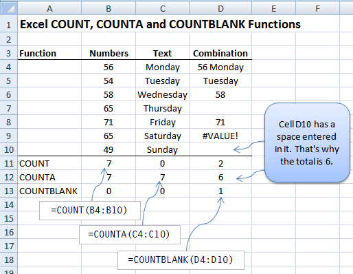
In rows 11-13 you can see the different results each formula returns depending on the Function used.
Enter your email address below to download the sample workbook.
By submitting your email address you agree that we can email you our Excel newsletter.
Other ways to COUNT in Excel
- Use a Pivot Table
- Use an Excel Table and insert a COUNT total
- Use the SUBTOTAL Function
Or, if you want to count cells that match specific criteria then take a look at the COUNTIF and COUNTIFS functions.
Usage notes
The COUNT function returns the count of numeric values in the list of supplied arguments. COUNT takes multiple arguments in the form value1, value2, value3, etc. Arguments can be individual hardcoded values, cell references, or ranges up to a total of 255 arguments. All numbers are counted, including negative numbers, percentages, dates, times, fractions, and formulas that return numbers. Empty cells and text values are ignored.
Examples
The COUNT function counts numeric values and ignores text values:
=COUNT(1,2,3) // returns 3
=COUNT(1,"a","b") // returns 1
=COUNT("apple",100,125,150,"orange") // returns 3
Typically, the COUNT function is used on a range. For example, to count numeric values in the range A1:A10:
=COUNT(A1:A100) // count numbers in A1:A10
In the example shown, COUNT is set up to count numbers in the range B5:B15:
=COUNT(B5:B15) // returns 6
COUNT returns 6, since there are 6 numeric values in the range B5:B15. Text values and blank cells are ignored. Note that dates and times are numbers, and therefore included in the count.
The COUNTA function works like the COUNT function, but COUNTA includes numbers and text in the count.
Functions for counting
- To count numbers only, use the COUNT function.
- To count numbers and text, use the COUNTA function.
- To count with one condition, use the COUNTIF function
- To count with multiple conditions, use the COUNTIFS function.
- To count empty cells, use the COUNTBLANK function.
Notes
- COUNT can handle up to 255 arguments.
- COUNT ignores the logical values TRUE and FALSE.
- COUNT ignores text values and empty cells.

Recently, I visited a friend who was working on a printout that was obviously generated by a spreadsheet application. It was a list of customer names and addresses sorted by ZIP Code, and my friend was manually counting how many customers were in each ZIP Code region. I hate to see users waste time doing something manually that could be done with software.
SEE: Google Workspace vs. Microsoft 365: A side-by-side analysis w/checklist (TechRepublic Premium)
Naturally, I had to stick my nose into the process and point out that there’s a much better way to get those numbers. In this tutorial, I’ll show you what I showed them: How to use Excel’s COUNTIF() function to return the number of times a specific value — in this case, ZIP Codes — occurs in a list. Along the way, you’ll also learn the basics of COUNTIF() so you can use this versatile function with your own work. Then, we’ll use SUBTOTAL() to count when filtering.
For this demonstration, I’m using Microsoft 365 on a Windows 10 64-bit system, but you can also use this function with earlier versions of Excel. Microsoft Excel for the web supports both of the functions we’ll be working with here.
If you’re interested in following along more closely, you can download our project demo file here.
Jump to:
- COUNTIF arguments
- How to use the COUNTIF function in Excel
- How do I count multiple items in Excel?
- How do I count filtered lists in Excel?
- Additional resources
COUNTIF arguments
Before we use either function, let’s look at the COUNTIF() arguments. COUNTIF() returns the number of cells that meet a specific condition that you specify. In our case, we’re counting the number of times a specific ZIP code occurs in a specified range.
COUNTIF() uses the following syntax:
COUNTIF(range,criteria)
where “range” identifies the list of values you are counting and “criteria” expresses the condition for counting.
Before we go any further, it’s important to know that COUNTIF() has one limitation. The criteria argument is limited to 255 characters when using a literal string value. It’s doubtful you’ll run into this limitation, but if you do, you can concatenate strings using the concatenation operator & to build a longer string.
Troubleshooting COUNTIF
If the COUNTIF() function returns nothing and you know the values exist, consider the following actions and tips:
- Be sure to delimit values: For example, “apples” will count the number of times the word apple appears in the referenced range; if you omit the quotation marks, it won’t work. Numeric values don’t require a delimiter, except for dates, which use the
#delimiter. - Check the values: Your referenced range may have an unnecessary space character before or after other characters. Use TRIM() to return only the values you want.
- Check if your file is open: If COUNTIF() refers to another workbook, that file must be open. Otherwise, the function returns the #VALUE! error.
- Take a closer look at your criteria text: COUNTIF() criteria values aren’t case sensitive. However, curly quotes in criteria will return an error, so if you’re pasting a value, be careful. In general, this shouldn’t be an issue.
- Don’t rely on cell formatting: COUNTIF() can’t count cells based on fill or font color values.
Now that you’re familiar with this function, let’s put it to use with a simple example.
How to use the COUNTIF function in Excel
Let’s start with a simple use of COUNTIF(). As you can see in Figure A, the function
=COUNTIF(Table1[ZIPS],10123)
returns the value of 2.
Figure A
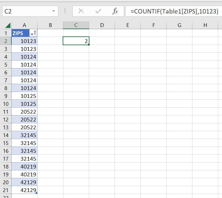
That’s because the ZIP Code value, 10123, occurs twice in the Table named Table1. If you’re not using a Table object, use the range reference as follows:
=COUNTIF(A2:A21,10123)
If you’re not familiar with structured referencing, Table1[ZIPS] might confuse you. The example data is formatted as an Excel Table object. Table1 is the Table object’s name and [ZIPS] is the column name.
Specifying a single ZIP Code is easy, but you’ll likely want to expand on this count by including all of them.
How do I count multiple items in Excel?
You can specify a literal value when using COUNTIF(), but the criteria argument supports a cell or range reference.
To demonstrate this function’s flexibility, we’ll count the number of occurrences of each ZIP Code in the sample data. Usually, ZIP Codes will accompany other address values such as name, address, city and state. We’re keeping our example simple on purpose, because those values are irrelevant when you’re counting only ZIP Code values.
SEE: Microsoft 365 Services Usage Policy (TechRepublic Premium)
If you’re using Microsoft 365, use the following expression to generate a unique list of sorted ZIP Code values (Figure B):
=SORT(UNIQUE(Table1[ZIPS]))
Figure B
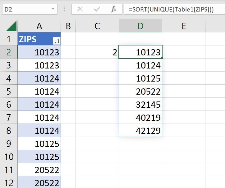
SORT() and UNIQUE() are both dynamic array functions, available only in Excel 365. In our example, there’s only one expression, which is in D2. However, the expression spills over into the cells below to fulfill the returned values as an array. If you get a spill error, there’s something blocking the array in the cells below the expression.
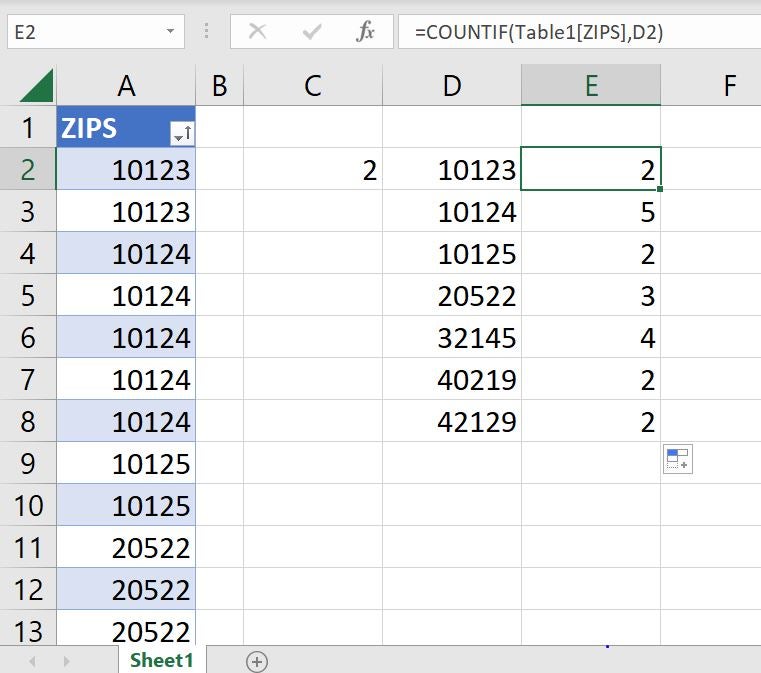
Once you have a unique list of ZIP Codes, you can use COUNTIF() to return the count of each ZIP Code value, as shown in Figure C, using
=COUNTIF(Table1[ZIPS],D2)
and copying it to the remaining cells.
Figure C
To learn more about dynamic arrays, you can read How to create a sorted unique list in an Excel spreadsheet.
How do I count multiple items in Excel pre-365?
For users who are using an earlier version of Excel than Excel 365, you’ll have to work a bit harder for the same results. If it’s important to you that the unique list of ZIP Codes is sorted, sort the source data before going any further.
To do so, you can simply click on any of the cells in column A and click the Sort Ascending button in the Sort & Filter group on the Data tab. Alternatively, you can click Sort & Filter in the Editing group on the Home tab.
To create a unique list of ZIP Codes from the values in column A, do the following:
- Click any group of cells in the dataset — in this example, we’ve selected A1:A21.
- Click the Data tab and then click Advanced in the Sort & Filter group.
- Click the Copy to Another Location option.
- Excel will display $A$1:$A$21 as the List Range. If it does not do this, you can fix it manually.
- Remove the Criteria Range if there is one.
- Click Copy To control and then click an unselected cell, such as G1.
- Check the Unique Records Only option (Figure D).
Figure D
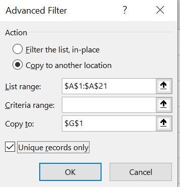
- Click OK.
This feature also copies the heading text from A1 and the formatting. There’s no way around either of these copies, but that’s okay, because neither interferes with our task.
At this point, all that’s left is the function for counting unique entries in column A based on entries in the unique list in column G. Now it’s time to enter the following function into cell H2:
=COUNTIF(Table1[ZIPS],G2)
You’ll then copy it to the remaining cells. As you can see in Figure E, this function returns the same counts as the first.
Figure E
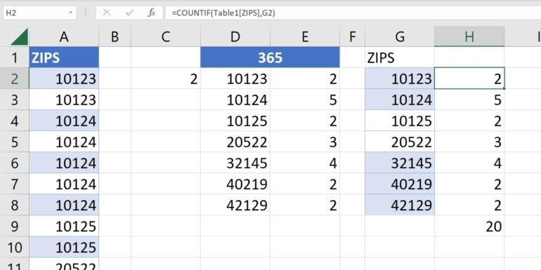
Did you notice the bold 20 in cell H9? That’s a SUM() function, which ensures the number of counted entries equals the number of original entries. Since we had 20 entries in our source data in column A, we’d expect the total number of unique entries counted to be the same.
COUNTIF() is a helpful way to count specific values in a list, but you may also run into situations where you want to count items in a filtered list. Let’s cover how to do that next.
How do I count filtered lists in Excel?
Using COUNTIF() works great in many situations, but what if you want a count based on the results of a filtered list? In this situation, the COUNTIF() function won’t work for you. The function will continue to return the correct results, but it won’t return the correct count for the filtered set. Instead, you’ll want to use the SUBTOTAL() function to count a filtered list.
Excel’s SUBTOTAL() function is rather special, as it accommodates filtering. Specifically, regardless of the mathematical calculation, this function evaluates only the values that make it to the filtered list. This function uses the following syntax:
SUBTOTAL(number,reference)
“Number” identifies the mathematical calculation and “reference” specifies the values. By default, number is 109, which is SUM(). Refer to Table A for a complete list of number values:
Table A
| Includes hidden rows | Excludes hidden rows | Function |
|---|---|---|
| 1 | 101 | AVERAGE |
| 2 | 102 | COUNT |
| 3 | 103 | COUNTA |
| 4 | 104 | MAX |
| 5 | 105 | MIN |
| 6 | 106 | PRODUCT |
| 7 | 107 | STDEV |
| 8 | 108 | STDEVP |
| 9 | 109 | SUM |
| 10 | 110 | VAR |
| 11 | 111 | VARP |
In the last section, COUNTIF() didn’t care whether the source data was a normal data range or a Table object. For this solution to work, you must work with a Table object. To convert a data range into a Table object, click anywhere inside the data range and press Ctrl + T and click OK to confirm the conversion. Doing so automatically displays a filter dropdown in the header cell.
Before we start filtering, we must add a special row to the Table as follows:
- Click anywhere inside the Table.
- Click the contextual Table Design tab.
- In the Table Style Options group, click the Total Row item (Figure F).
Figure F
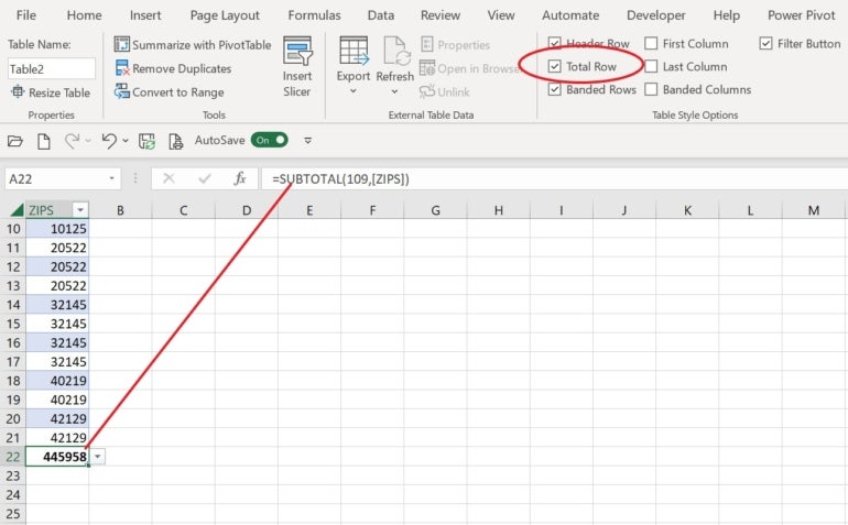
As you can see in Figure F, this row defaults to a SUBTOTAL() function that totals values by default. In this case, we don’t want a total but rather a count. To change the SUBTOTAL() function’s argument, click A22 and choose Count from the dropdown list shown in Figure G.
Figure G
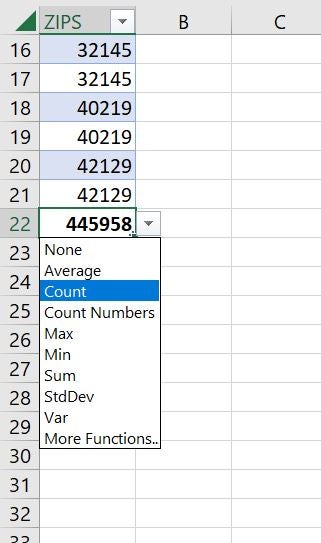
As you can see, there are many different functions you can choose. Figure H shows the count, which is 20.
Figure H
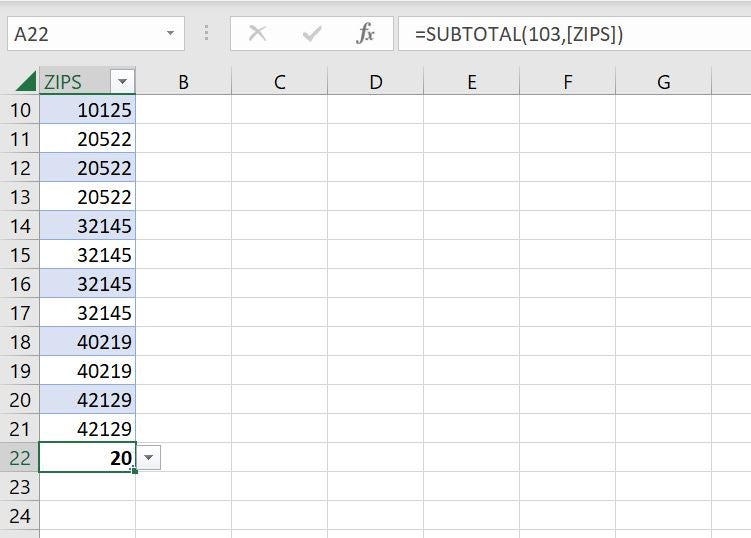
The original SUBTOTAL() function’s first argument is 109, which represents SUM(). When you change the total function to Count, SUBTOTAL() updates that argument to 103, which represents COUNT().
Start the filtering process
Once the total row is in place and displaying the count, you’re ready to begin filtering. To start, try clicking the filtering dropdown in A1 and do the following:
- Uncheck (Select All).
- Check the 10125 option (Figure I).
Figure I
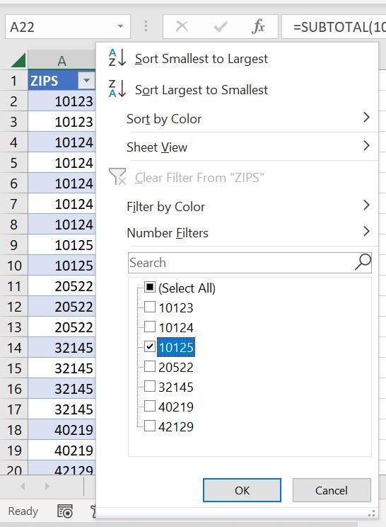
- Click OK.
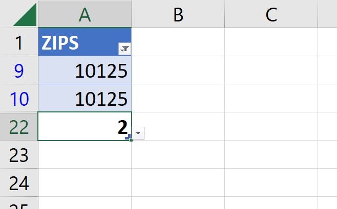
As you can see in Figure J, the filtered set includes two items, and the SUBTOTAL() function now returns two instead of 20. This function is special because, unlike other functions, SUBTOTAL() updates when you apply a filter.
Figure J
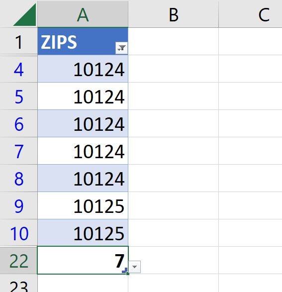
Let’s try it again, only this time, check two ZIP Codes (Figure K).
Figure K
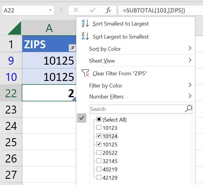
As you can see in Figure L, SUBTOTAL() returns the count of both ZIP Code values, which is 7. SUBTOTAL() is flexible enough to handle any filter you apply using the advanced filter feature.
Figure L
Additional resources
Whether you use COUNTIF() or SUBTOTAL() via a Table object’s total row, counting values is easy work. To learn more about counting, this other TechRepublic tutorial can help: How to use the UNIQUE() function to return a count of unique values in Excel.
Read next: The 8 best alternatives to Microsoft Project (Free & Paid) (TechRepublic)