Count in excel by name - Word и Excel - помощь в работе с программами

Ways to count cells in a range of data

Select the cell where you want the result to appear.
On the Formulas tab, click More Functions, point to Statistical, and then click one of the following functions: COUNTA: To count cells that are not empty.
Select the range of cells that you want, and then press RETURN.

Contents

1 How do I count a list of names in Excel?
2 How do I count text names in Excel?
3 How do I count how many times a name appears in Excel?
4 How do I count the same name in Excel cell?
5 How do I count numbers in Excel?
6 How do you count text in a cell?
7 How do I count the number of items in a column in Excel?
8 How do I count only duplicate names in Excel?
9 How do I count text in Excel without duplicates?
10 How do I count multiple values in Excel?
11 Can you count characters in Excel?
12 How do I count partial text in Excel?
13 How do you count cells with only values?

How do I count a list of names in Excel?

Counting items in an Excel list

Sort the list by the appropriate column.
Use Advanced Filter to create a list of the unique entries in the appropriate column.
Use the =Countif function to count the number of times each unique entry appears in the original list.

How do I count text names in Excel?

How to Count Text in Excel

If you want to learn how to count text in Excel, you need to use function COUNTIF with the criteria defined using wildcard *, with the formula: =COUNTIF(range;”*”) .
Text Cells can be easily found in Excel using COUNTIF or COUNTIFS functions.

How do I count how many times a name appears in Excel?

Count a Specific Word in a Range using COUNTIF

Select the cell that you want to write the count in (cell D3 in our case).
In this cell, type the formula: =COUNTIF(A2:A10,”Peter”)
Press the return key.

How do I count the same name in Excel cell?

How to Count the Total Number of Duplicates in a Column

Go to cell B2 by clicking on it.
Assign the formula =IF(COUNTIF($A$2:A2,A2)>1,”Yes”,””) to cell B2.
Press Enter.
Drag down the formula from B2 to B8.
Select cell B9.
Assign the formula =COUNTIF(B2:B8,”Yes”) to cell B9.
Hit Enter.

How do I count numbers in Excel?

Use the COUNT function to get the number of entries in a number field that is in a range or array of numbers. For example, you can enter the following formula to count the numbers in the range A1:A20: =COUNT(A1:A20). In this example, if five of the cells in the range contain numbers, the result is 5.

How do you count text in a cell?

To use the function, enter =LEN(cell) in the formula bar, then press Enter on your keyboard. Multiple cells: To apply the same formula to multiple cells, enter the formula in the first cell and then drag the fill handle down (or across) the range of cells.

How do I count the number of items in a column in Excel?

Count Numbers, All Data, or Blank Cells

Enter the sample data on your worksheet.
In cell A7, enter an COUNT formula, to count the numbers in column A: =COUNT(A1:A5)
Press the Enter key, to complete the formula.
The result will be 3, the number of cells that contain numbers.

How do I count only duplicate names in Excel?

Part 2: Count Duplicate Values Once with Case Insensitive
This time we count number with case insensitive. Step 1: In B2 enter the formula =SUMPRODUCT((A2:A11<>””)/COUNTIF(A2:A11,A2:A11&””)). Step 2: Press Enter directly to get result.

How do I count text in Excel without duplicates?

You can do this efficiently by combining SUM and COUNTIF functions. A combo of two functions can count unique values without duplication. Below is the syntax: =SUM(IF(1/COUNTIF(data, data)=1,1,0)).

How do I count multiple values in Excel?

To get a count of values between two values, we need to use multiple criteria in the COUNTIF function. You can also use a combination of cells references and operators (where the operator is entered directly in the formula). When you combine an operator and a cell reference, the operator is always in double quotes.

Can you count characters in Excel?

When you need to count the characters in cells, use the LEN function. The function counts letters, numbers, characters, and all spaces.To use the function, enter =LEN(cell) in the formula bar and press Enter.

How do I count partial text in Excel?

Select a blank cell you will place the counting result at, type the formula =COUNTIF(A1:A16,”*Anne*”) (A1:A16 is the range you will count cells, and Anne is the certain partial string) into it, and press the Enter key. And then it counts out the total number of cells containing the partial string.

How do you count cells with only values?

Use the COUNTA function function to count only cells in a range that contain values. When you count cells, sometimes you want to ignore any blank cells because only cells with values are meaningful to you. For example, you want to count the total number of salespeople who made a sale (column D).

Источник

Count Names in Excel (Table of Contents)

Overview of Count Names in Excel
How to Count Names in Excel?

Overview of Count Names in Excel

COUNT is an in-built function in MS Excel that will count the number of cells that contain numbers. It comes under the statistical function category and is used to return an integer as output. There are many ways to count the cells in the given range with several user criteria. Examples are COUNTIF, DCOUNT, COUNTA, etc.

Formula: There are many value parameters in the simple count function, which will count all cells which contain numbers.

There are some specific in-built Count functions which are listed below:

COUNT: It will count the number of cells that contain the numbers.
COUNTIF: It will count the number of cells containing the numbers and satisfy the user’s criteria.
DCOUNT: It will count the cells containing some number in the selected database and satisfy the user criteria.
DCOUNTA: It will count the non-blank cells in the selected database which satisfy the user criteria.

How to Count Names in Excel?

Counting Names in excel is very simple and easy. So, here are some examples that can help you to Count Names in Excel.

You can download this Count Names Excel Template here – Count Names Excel Template

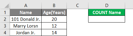
Example #1 – Count Name which has Age Data

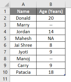
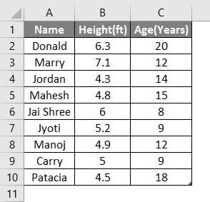
Let’s assume a user has some people’s data like Name and Age, where the user wants to calculate the count of the name with age data in the table.

Let’s see how we can do this with the count function.

Step 1: Open MS Excel from the start menu >> Go to Sheet1, where the user keeps the data.

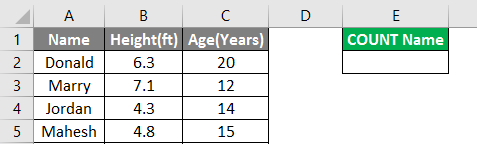
Step 2: Now create headers for the Count name where the user wants the count name, which has age data.

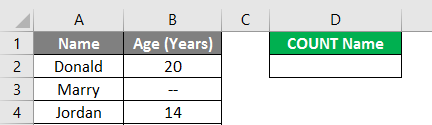
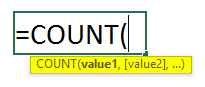
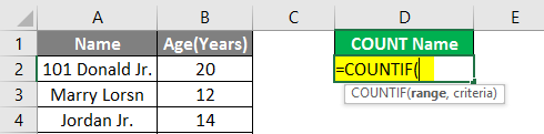
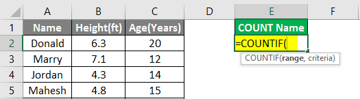
Step 3: Now calculate the count of a name in the given data by the Count function>> use the equal sign to calculate >> Write in D2 Cell and use COUNT>> “=COUNT (”

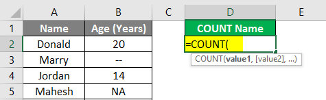
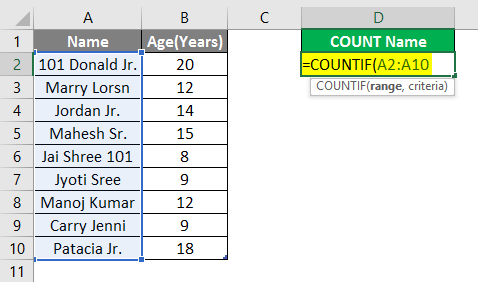
Step 4: Now, it will ask for the value1 which are given in B2 to B10 cell >> select B2 to B10 cell >> “=COUNT (B2: A10)”

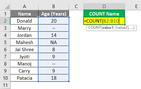
Step 5: Now press the Enter key.

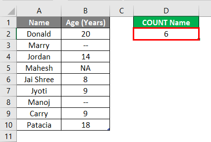
Summary of Example #1: The user wants to calculate the name count, which has age data in the table. So, 6 names in the above example have age data in the table.

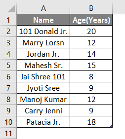
Example #2 – Count Name which has Some Common String

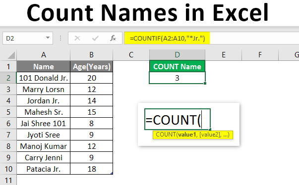
Let’s assume a user has some people’s personal data like Name and Age, where the user wants to calculate the count of the name with the “Jr.” string common in their name. Let’s see how we can do this with the COUNTIF function.

Step 1: Open MS Excel from the start menu >> Go to Sheet2, where the user keeps the data.

Step 2: Create a header for the Count name, with a “Jr.” string common in their name.

Step 3: Now calculate the count of a name in the given data by the COUNTIF function>> use the equal sign to calculate >> Write in D2 Cell and use COUNTIF>> “=COUNTIF (”

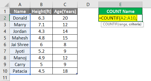
Step 4: Now, it will ask for value1 which are given in A2 to A10 cell >> select A2 to A10 cell >> “=COUNTIF (A2: A10,”

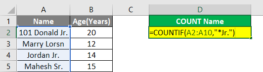
Step 5: Now it will ask for criteria which are to search only for the “Jr.” string in the name >>so write in D2 cell >> “=COUNTIF (A2: A10,” *Jr.”)”

Step 6: Now press the Enter key.

Summary of Example #2: The user wants to count the name with the “Jr.” string common in their name in the table. So, three names in the above example have the “Jr.” string in their name.

Example #3 – Number of Letters with Ending a Specific String

Let’s assume a user wants to count the names with 5 letters and the “ry” string common in their name. Let’s see how we can do this with the COUNTIF function.

Step 1: Open MS Excel from the start menu >> Go to Sheet3, where the user keeps the data.

Step 2: Create a header for the Count name, with 5 letters and a “ry” string common in their name.

Step 3: Now calculate the count of a name in the given data by the COUNTIF function>> use the equal sign to calculate >> Write in E2 Cell and use COUNTIF>> “=COUNTIF (”

Step 4: Now, it will ask for value1 which are given in A2 to A10 cell >> select A2 to A10 cell >> “=COUNTIF (A2: A10,”

Step 5: Now it will ask for criteria which are to search only for the “ry” string in the name with 5 letters>>so write in E2 cell >> “=COUNTIF (A2: A10,”???ry”)”

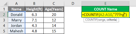
Step 6: Now press the Enter key.

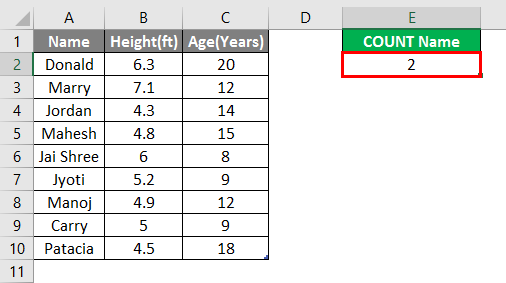
Summary of Example #3: The user wants to count the names with 5 letters in the Name and the “ry” string common in their name in the table. So, 2 names in the above example have a “ry” string in their name with five letters.

Things to Remember About Count Names in Excel

The Count function comes under the statistical function category and is used to return an integer as output.
If a cell contains any value that is not numeric, like text or #NA, it will not be counted by the count function.
The asterisk (*) matches any set of characters in the COUNTIF criteria.
The question mark (?) is used as the wildcard character to match any single character in the criteria of the function.
In the criteria, a user can use greater than “>,” less than “<” or equal to the “=” symbol to create criteria in the function. As an example, “=COUNTIF (A2:A5,” >=10″)” here as the output will return the count of the cell, which has a value greater than or equal to 10.

Example 1: Count Cells with Exact Name

We can use the following formula to count the number of cells in column A that contain the exact name “Bob Johnson”:

=COUNTIF(A2:A11, "Bob Johnson")

The following screenshot shows how to use this formula in practice:

We can see that there are 2 cells that contain “Bob Johnson” as the exact name.

Example 2: Count Cells with Partial Name

We can use the following formula to count the number of cells in column A that contain “Johnson” anywhere in the name:

=COUNTIF(A2:A11, "*Johnson*")

The following screenshot shows how to use this formula in practice:

We can see that there are 4 cells that contain “Johnson” somewhere in the name.

Example 3: Count Cells with One of Several Names

We can use the following formula to count the number of cells in column A that contain “Johnson” or “Smith” somewhere in the name:

=COUNTIF(A2:A11, "*Johnson*") + COUNTIF(A2:A11, "*Smith*")

The following screenshot shows how to use this formula in practice:

We can see that there are 6 cells that contain either “Johnson” or “Smith” somewhere in the name.

Additional Resources

The following tutorials explain how to perform other common tasks in Excel:

How to Count Specific Words in Excel
How to Count Unique Values by Group in Excel
How to Use COUNTIF with Multiple Ranges in Excel

Источник

Counting is an integral part of data analysis, whether you are tallying the head count of a department in your organization or the number of units that were sold quarter-by-quarter. Excel provides multiple techniques that you can use to count cells, rows, or columns of data. To help you make the best choice, this article provides a comprehensive summary of methods, a downloadable workbook with interactive examples, and links to related topics for further understanding.

Download our examples

You can download an example workbook that gives examples to supplement the information in this article. Most sections in this article will refer to the appropriate worksheet within the example workbook that provides examples and more information.

Download examples to count values in a spreadsheet

Simple counting
- Use AutoSum
- Add a Subtotal row
- Count cells in a list or Excel table column by using the SUBTOTAL function
Counting based on one or more conditions
- Video: Use the COUNT, COUNTIF, and COUNTA functions
- Count cells in a range by using the COUNT function
- Count cells in a range based on a single condition by using the COUNTIF function
- Count cells in a column based on single or multiple conditions by using the DCOUNT function
- Count cells in a range based on multiple conditions by using the COUNTIFS function
- Count based on criteria by using the COUNT and IF functions together
- Count how often multiple text or number values occur by using the SUM and IF functions together
- Count cells in a column or row in a PivotTable
Counting when your data contains blank values
- Count nonblank cells in a range by using the COUNTA function
- Count nonblank cells in a list with specific conditions by using the DCOUNTA function
- Count blank cells in a contiguous range by using the COUNTBLANK function
- Count blank cells in a non-contiguous range by using a combination of SUM and IF functions
Counting unique occurrences of values
- Count the number of unique values in a list column by using Advanced Filter
- Count the number of unique values in a range that meet one or more conditions by using IF, SUM, FREQUENCY, MATCH, and LEN functions
Special cases (count all cells, count words)
- Count the total number of cells in a range by using ROWS and COLUMNS functions
- Count words in a range by using a combination of SUM, IF, LEN, TRIM, and SUBSTITUTE functions
Displaying calculations and counts on the status bar

Simple counting

You can count the number of values in a range or table by using a simple formula, clicking a button, or by using a worksheet function.

Excel can also display the count of the number of selected cells on the Excel status bar. See the video demo that follows for a quick look at using the status bar. Also, see the section Displaying calculations and counts on the status bar for more information. You can refer to the values shown on the status bar when you want a quick glance at your data and don’t have time to enter formulas.

Video: Count cells by using the Excel status bar

Watch the following video to learn how to view count on the status bar.

Use AutoSum

Use AutoSum by selecting a range of cells that contains at least one numeric value. Then on the Formulas tab, click AutoSum > Count Numbers.

Excel returns the count of the numeric values in the range in a cell adjacent to the range you selected. Generally, this result is displayed in a cell to the right for a horizontal range or in a cell below for a vertical range.

Top of Page

Add a Subtotal row

You can add a subtotal row to your Excel data. Click anywhere inside your data, and then click Data > Subtotal.

Note: The Subtotal option will only work on normal Excel data, and not Excel tables, PivotTables, or PivotCharts.

Also, refer to the following articles:

Outline (group) data in a worksheet
Insert subtotals in a list of data in a worksheet

Top of Page

Count cells in a list or Excel table column by using the SUBTOTAL function

Use the SUBTOTAL function to count the number of values in an Excel table or range of cells. If the table or range contains hidden cells, you can use SUBTOTAL to include or exclude those hidden cells, and this is the biggest difference between SUM and SUBTOTAL functions.

The SUBTOTAL syntax goes like this:

SUBTOTAL(function_num,ref1,[ref2],…)

To include hidden values in your range, you should set the function_num argument to 2.

To exclude hidden values in your range, set the function_num argument to 102.

Top of Page

Counting based on one or more conditions

You can count the number of cells in a range that meet conditions (also known as criteria) that you specify by using a number of worksheet functions.

Video: Use the COUNT, COUNTIF, and COUNTA functions

Watch the following video to see how to use the COUNT function and how to use the COUNTIF and COUNTA functions to count only the cells that meet conditions you specify.

Top of Page

Count cells in a range by using the COUNT function

Use the COUNT function in a formula to count the number of numeric values in a range.

In the above example, A2, A3, and A6 are the only cells that contains numeric values in the range, hence the output is 3.

Note: A7 is a time value, but it contains text (a.m.), hence COUNT does not consider it a numerical value. If you were to remove a.m. from the cell, COUNT will consider A7 as a numerical value, and change the output to 4.

Top of Page

Count cells in a range based on a single condition by using the COUNTIF function

Use the COUNTIF function function to count how many times a particular value appears in a range of cells.

Top of Page

Count cells in a column based on single or multiple conditions by using the DCOUNT function

DCOUNT function counts the cells that contain numbers in a field (column) of records in a list or database that match conditions that you specify.

In the following example, you want to find the count of the months including or later than March 2016 that had more than 400 units sold. The first table in the worksheet, from A1 to B7, contains the sales data.

DCOUNT uses conditions to determine where the values should be returned from. Conditions are typically entered in cells in the worksheet itself, and you then refer to these cells in the criteria argument. In this example, cells A10 and B10 contain two conditions—one that specifies that the return value must be greater than 400, and the other that specifies that the ending month should be equal to or greater than March 31st, 2016.

You should use the following syntax:

=DCOUNT(A1:B7,»Month ending»,A9:B10)

DCOUNT checks the data in the range A1 through B7, applies the conditions specified in A10 and B10, and returns 2, the total number of rows that satisfy both conditions (rows 5 and 7).

Top of Page

Count cells in a range based on multiple conditions by using the COUNTIFS function

The COUNTIFS function is similar to the COUNTIF function with one important exception: COUNTIFS lets you apply criteria to cells across multiple ranges and counts the number of times all criteria are met. You can use up to 127 range/criteria pairs with COUNTIFS.

The syntax for COUNTIFS is:

COUNTIFS(criteria_range1, criteria1, [criteria_range2, criteria2],…)

See the following example:

Top of Page

Count based on criteria by using the COUNT and IF functions together

Let’s say you need to determine how many salespeople sold a particular item in a certain region or you want to know how many sales over a certain value were made by a particular salesperson. You can use the IF and COUNT functions together; that is, you first use the IF function to test a condition and then, only if the result of the IF function is True, you use the COUNT function to count cells.

Notes:

The formulas in this example must be entered as array formulas. If you have opened this workbook in Excel for Windows or Excel 2016 for Mac and want to change the formula or create a similar formula, press F2, and then press Ctrl+Shift+Enter to make the formula return the results you expect. In earlier versions of Excel for Mac, use +Shift+Enter.
For the example formulas to work, the second argument for the IF function must be a number.

Top of Page

Count how often multiple text or number values occur by using the SUM and IF functions together

In the examples that follow, we use the IF and SUM functions together. The IF function first tests the values in some cells and then, if the result of the test is True, SUM totals those values that pass the test.

Example 1

The above function says if C2:C7 contains the values Buchanan and Dodsworth, then the SUM function should display the sum of records where the condition is met. The formula finds three records for Buchanan and one for Dodsworth in the given range, and displays 4.

Example 2

The above function says if D2:D7 contains values lesser than $9000 or greater than $19,000, then SUM should display the sum of all those records where the condition is met. The formula finds two records D3 and D5 with values lesser than $9000, and then D4 and D6 with values greater than $19,000, and displays 4.

Example 3

The above function says if D2:D7 has invoices for Buchanan for less than $9000, then SUM should display the sum of records where the condition is met. The formula finds that C6 meets the condition, and displays 1.

Important: The formulas in this example must be entered as array formulas. That means you press F2 and then press Ctrl+Shift+Enter. In earlier versions of Excel for Mac use +Shift+Enter.

See the following Knowledge Base articles for additional tips:

XL: Using SUM(IF()) As an Array Function Instead of COUNTIF() with AND
XL: How to Count the Occurrences of a Number or Text in a Range

Top of Page

Count cells in a column or row in a PivotTable

A PivotTable summarizes your data and helps you analyze and drill down into your data by letting you choose the categories on which you want to view your data.

You can quickly create a PivotTable by selecting a cell in a range of data or Excel table and then, on the Insert tab, in the Tables group, clicking PivotTable.

Let’s look at a sample scenario of a Sales spreadsheet, where you can count how many sales values are there for Golf and Tennis for specific quarters.

Note: For an interactive experience, you can run these steps on the sample data provided in the PivotTable sheet in the downloadable workbook.

Enter the following data in an Excel spreadsheet.
Select A2:C8
Click Insert > PivotTable.
In the Create PivotTable dialog box, click Select a table or range, then click New Worksheet, and then click OK.

An empty PivotTable is created in a new sheet.
In the PivotTable Fields pane, do the following:
1. Drag Sport to the Rows area.
2. Drag Quarter to the Columns area.
3. Drag Sales to the Values area.
4. Repeat step c.
  
  The field name displays as SumofSales2 in both the PivotTable and the Values area.
  
  At this point, the PivotTable Fields pane looks like this:
5. In the Values area, click the dropdown next to SumofSales2 and select Value Field Settings.
6. In the Value Field Settings dialog box, do the following:
  1. In the Summarize value field by section, select Count.
  2. In the Custom Name field, modify the name to Count.
  3. Click OK.
The PivotTable displays the count of records for Golf and Tennis in Quarter 3 and Quarter 4, along with the sales figures.

Top of Page

Counting when your data contains blank values

You can count cells that either contain data or are blank by using worksheet functions.

Count nonblank cells in a range by using the COUNTA function

Use the COUNTA function function to count only cells in a range that contain values.

When you count cells, sometimes you want to ignore any blank cells because only cells with values are meaningful to you. For example, you want to count the total number of salespeople who made a sale (column D).

COUNTA ignores the blank values in D3, D4, D8, and D11, and counts only the cells containing values in column D. The function finds six cells in column D containing values and displays 6 as the output.

Top of Page

Count nonblank cells in a list with specific conditions by using the DCOUNTA function

Use the DCOUNTA function to count nonblank cells in a column of records in a list or database that match conditions that you specify.

The following example uses the DCOUNTA function to count the number of records in the database that is contained in the range A1:B7 that meet the conditions specified in the criteria range A9:B10. Those conditions are that the Product ID value must be greater than or equal to 2000 and the Ratings value must be greater than or equal to 50.

DCOUNTA finds two rows that meet the conditions- rows 2 and 4, and displays the value 2 as the output.

Top of Page

Count blank cells in a contiguous range by using the COUNTBLANK function

Use the COUNTBLANK function function to return the number of blank cells in a contiguous range (cells are contiguous if they are all connected in an unbroken sequence). If a cell contains a formula that returns empty text («»), that cell is counted.

When you count cells, there may be times when you want to include blank cells because they are meaningful to you. In the following example of a grocery sales spreadsheet. suppose you want to find out how many cells don’t have the sales figures mentioned.

Note: The COUNTBLANK worksheet function provides the most convenient method for determining the number of blank cells in a range, but it doesn’t work very well when the cells of interest are in a closed workbook or when they do not form a contiguous range. The Knowledge Base article XL: When to Use SUM(IF()) instead of CountBlank() shows you how to use a SUM(IF()) array formula in those cases.

Top of Page

Count blank cells in a non-contiguous range by using a combination of SUM and IF functions

Use a combination of the SUM function and the IF function. In general, you do this by using the IF function in an array formula to determine whether each referenced cell contains a value, and then summing the number of FALSE values returned by the formula.

See a few examples of SUM and IF function combinations in an earlier section Count how often multiple text or number values occur by using the SUM and IF functions together in this topic.

Top of Page

Counting unique occurrences of values

You can count unique values in a range by using a PivotTable, COUNTIF function, SUM and IF functions together, or the Advanced Filter dialog box.

Count the number of unique values in a list column by using Advanced Filter

Use the Advanced Filter dialog box to find the unique values in a column of data. You can either filter the values in place or you can extract and paste them to a new location. Then you can use the ROWS function to count the number of items in the new range.

To use Advanced Filter, click the Data tab, and in the Sort & Filter group, click Advanced.

The following figure shows how you use the Advanced Filter to copy only the unique records to a new location on the worksheet.

In the following figure, column E contains the values that were copied from the range in column D.

Notes:

If you filter your data in place, values are not deleted from your worksheet — one or more rows might be hidden. Click Clear in the Sort & Filter group on the Data tab to display those values again.
If you only want to see the number of unique values at a quick glance, select the data after you have used the Advanced Filter (either the filtered or the copied data) and then look at the status bar. The Count value on the status bar should equal the number of unique values.

For more information, see Filter by using advanced criteria

Top of Page

Count the number of unique values in a range that meet one or more conditions by using IF, SUM, FREQUENCY, MATCH, and LEN functions

Use various combinations of the IF, SUM, FREQUENCY, MATCH, and LEN functions.

For more information and examples, see the section «Count the number of unique values by using functions» in the article Count unique values among duplicates.

Top of Page

Special cases (count all cells, count words)

You can count the number of cells or the number of words in a range by using various combinations of worksheet functions.

Count the total number of cells in a range by using ROWS and COLUMNS functions

Suppose you want to determine the size of a large worksheet to decide whether to use manual or automatic calculation in your workbook. To count all the cells in a range, use a formula that multiplies the return values using the ROWS and COLUMNS functions. See the following image for an example:

Top of Page

Count words in a range by using a combination of SUM, IF, LEN, TRIM, and SUBSTITUTE functions

You can use a combination of the SUM, IF, LEN, TRIM, and SUBSTITUTE functions in an array formula. The following example shows the result of using a nested formula to find the number of words in a range of 7 cells (3 of which are empty). Some of the cells contain leading or trailing spaces — the TRIM and SUBSTITUTE functions remove these extra spaces before any counting occurs. See the following example:

Now, for the above formula to work correctly, you have to make this an array formula, otherwise the formula returns the #VALUE! error. To do that, click on the cell that has the formula, and then in the Formula bar, press Ctrl + Shift + Enter. Excel adds a curly bracket at the beginning and the end of the formula, thus making it an array formula.

For more information on array formulas, see Overview of formulas in Excel and Create an array formula.

Top of Page

Displaying calculations and counts on the status bar

When one or more cells are selected, information about the data in those cells is displayed on the Excel status bar. For example, if four cells on your worksheet are selected, and they contain the values 2, 3, a text string (such as «cloud»), and 4, all of the following values can be displayed on the status bar at the same time: Average, Count, Numerical Count, Min, Max, and Sum. Right-click the status bar to show or hide any or all of these values. These values are shown in the illustration that follows.

Top of Page

Need more help?

You can always ask an expert in the Excel Tech Community or get support in the Answers community.

Источник

In this example, the goal is to count cells that contain a specific substring. This problem can be solved with the SUMPRODUCT function or the COUNTIF function. Both approaches are explained below. The SUMPRODUCT version can also perform a case-sensitive count.

COUNTIF function

The COUNTIF function counts cells in a range that meet supplied criteria. For example, to count the number of cells in a range that contain «apple» you can use COUNTIF like this:

=COUNTIF(range,"apple") // equal to "apple"

Notice this is an exact match. To be included in the count, a cell must contain «apple» and only «apple». If a cell contains any other characters, it will not be counted.

In the example shown, the goal is to count cells that contain specific text, meaning the text is a substring that can be anywhere in the cell. To do this, we need to use the asterisk (*) character as a wildcard. To count cells that contain the substring «apple», we can use a formula like this:

=COUNTIF(range,"*apple*")

The asterisk (*) wildcard matches zero or more characters of any kind, so this formula will count cells that contain «apple» anywhere in the cell. The formulas used in the worksheet shown follow the same pattern:

=COUNTIF(B5:B15,"*a*") // contains "a"
=COUNTIF(B5:B15,"*2*") // contains "2"
=COUNTIF(B5:B15,"*-S*") // contains "-s"
=COUNTIF(B5:B15,"*x*") // contains "x"

You can easily adjust this formula to use a cell reference in criteria. For example, if A1 contains the text you want to match, you can use:

=COUNTIF(range,"*"&A1&"*")

Inside COUNTIF, the two asterisks are concatenated to the value in A1, and the formula works as before. The COUNTIF function supports three different wildcards, see this page for more details.

Note the COUNTIF formula above won’t work if you are looking for a particular number and cells contain numeric data. This is because the wildcard automatically causes COUNTIF to look for text only (i.e. to look for «2» instead of just 2). Because a text value won’t ever be found in a true number, COUNTIF will return zero. In addition, COUNTIF is not case-sensitive, so you can’t perform a case-sensitive count. The SUMPRODUCT alternative below can handle both cases.

SUMPRODUCT function

Another way to solve this problem is with the SUMPRODUCT function and Boolean algebra. This approach has the benefit of being case-sensitive if needed. In addition, you can use this technique to find a number inside of a number, something you can’t do with COUNTIF.

To count cells that contain specific text with SUMPRODUCT, you can use the SEARCH function. SEARCH returns the position of text in a text string as a number. For example, the formula below returns 6 since the «a» appears first as the sixth character in the string:

=SEARCH( "a","The cat sat") // returns 6

If the text is not found, SEARCH returns a #VALUE! error:

=SEARCH( "x","The cat sat") // returns #VALUE!

To count cells that contain «a» in the worksheet shown with SUMPRODUCT, you can use the ISNUMBER and SEARCH functions like this:

=SUMPRODUCT(--ISNUMBER(SEARCH("a",B5:B15)))

Working from the inside out, the logical test inside SUMPRODUCT is based on SEARCH:

SEARCH("a",B5:B15)

Because the range B5:B15 contains 11 cells, the result from SEARCH is an array with 11 results:

{1;1;1;1;2;2;#VALUE!;#VALUE!;#VALUE!;#VALUE!;#VALUE!}

In this array, numbers indicate the position of «a» in cells where «a» is found. The #VALUE! errors indicate cells where «a» was not found. To convert these results into a simple array of TRUE and FALSE values, the SEARCH function is nested in the ISNUMBER function:

ISNUMBER(SEARCH("a",B5:B15))

ISNUMBER returns TRUE for any number and FALSE for errors. SEARCH delivers the array of results to ISNUMBER, and ISNUMBER converts the results to an array that contains only TRUE and FALSE values:

{TRUE;TRUE;TRUE;TRUE;TRUE;TRUE;FALSE;FALSE;FALSE;FALSE;FALSE}

In this array, TRUE corresponds to cells that contain «a» and FALSE corresponds to cells that do not contain «a». We want to count these results, but we first need to convert the TRUE and FALSE values to their numeric equivalents, 1 and 0. To do this, we use a double negative (—):

--ISNUMBER(SEARCH("a",B5:B15))

The result inside of SUMPRODUCT looks like this:

=SUMPRODUCT({1;1;1;1;1;1;0;0;0;0;0}) // returns 6

With a single array to process, SUMPRODUCT sums the array and returns 6 as a final result.

One benefit of this formula is it will find a number inside a numeric value. In addition, there is no need to use wildcards to indicate position, because SEARCH will automatically look through all text in a cell.

Case-sensitive option

For a case-sensitive count, you can replace the SEARCH function with the FIND function like this:

=SUMPRODUCT(--(ISNUMBER(FIND(text,range))))

The FIND function works just like the SEARCH function, but is case-sensitive. You can use a formula like this to count cells that contain «APPLE» and not «apple». This example provides more detail.

Источник

How do I count a list of names in Excel?

How do I count text names in Excel?

How do I count how many times a name appears in Excel?

How do I count the same name in Excel cell?

How do I count numbers in Excel?

How do you count text in a cell?

How do I count the number of items in a column in Excel?

How do I count only duplicate names in Excel?

How do I count text in Excel without duplicates?

How do I count multiple values in Excel?

Can you count characters in Excel?

How do I count partial text in Excel?

How do you count cells with only values?

Overview of Count Names in Excel

How to Count Names in Excel?

Example #1 – Count Name which has Age Data

Example #2 – Count Name which has Some Common String

Example #3 – Number of Letters with Ending a Specific String

Things to Remember About Count Names in Excel

Recommended Articles

Example 1: Count Cells with Exact Name

Example 2: Count Cells with Partial Name

Example 3: Count Cells with One of Several Names

Additional Resources

Download our examples

In this article

Simple counting

Video: Count cells by using the Excel status bar

Use AutoSum

Add a Subtotal row

Count cells in a list or Excel table column by using the SUBTOTAL function

Counting based on one or more conditions

Video: Use the COUNT, COUNTIF, and COUNTA functions

Count cells in a range by using the COUNT function

Count cells in a range based on a single condition by using the COUNTIF function

Count cells in a column based on single or multiple conditions by using the DCOUNT function

Count cells in a range based on multiple conditions by using the COUNTIFS function

Count based on criteria by using the COUNT and IF functions together

Count how often multiple text or number values occur by using the SUM and IF functions together

Count cells in a column or row in a PivotTable

Counting when your data contains blank values

Count nonblank cells in a range by using the COUNTA function

Count nonblank cells in a list with specific conditions by using the DCOUNTA function

Count blank cells in a contiguous range by using the COUNTBLANK function

Count blank cells in a non-contiguous range by using a combination of SUM and IF functions

Counting unique occurrences of values

Count the number of unique values in a list column by using Advanced Filter

Count the number of unique values in a range that meet one or more conditions by using IF, SUM, FREQUENCY, MATCH, and LEN functions

Special cases (count all cells, count words)

Count the total number of cells in a range by using ROWS and COLUMNS functions

Count words in a range by using a combination of SUM, IF, LEN, TRIM, and SUBSTITUTE functions

Displaying calculations and counts on the status bar

Need more help?

COUNTIF function

SUMPRODUCT function

Case-sensitive option