Count in excel but not duplicates - Word и Excel - помощь в работе с программами

Data analysis usually involves large data sets, and at some point, one may need to find out the number of values that appear only once in the dataset. In this case, you will be counting without duplicates. Unique values are values that appear only once in a dataset.

If you are faced with mountains of data, then counting without duplicates might be very arduous. More so, Excel does not have a special formula for counting without duplicates. However, there is always a way out! This tutorial will serve as a guide on how to count unique and distinct values without duplicating them.

Take a look at the numbers in the table above; the unique values are not duplicated. They don’t appear more than once. Whereas, distinct values are the different numbers in the collection. In the table below, we have separated the unique values from distinct values.

1. Using the array COUNTIF formula

The COUNTIF function counts the frequency of occurrence of each value within the range. To get the number of the unique values, you have to sum them up. You can do this efficiently by combining SUM and COUNTIF functions. A combo of two functions can count unique values without duplication.

Below is the syntax:

=SUM(IF(COUNTIF(data, data)=1,1,0)).

The formula contains three separate functions – SUM, IF, and COUNTIF.

COUNTIF function» counts how many times a particular number appears within the range.

«IF function» analysis the results returned by the «COUNTIF» function. It maintains the 1’s for unique values and replaces other values with «0.»

Note: Always press Ctrl + Shift + Enter when entering your array formula.

CTRL+SHIFT+ENTER allow excel to recognize the formula as an array function. unique value= =SUM(IF(COUNTIF(A2:A10, A2:A10)=1,1,0))

Alternatively, you can use the SUMPRODUCT formula to avoid the use of CTRL+SHIFT+ENTER.

Below is the syntax:

=SUMPRODUCT(1/COUNTIF(range, criteria)).

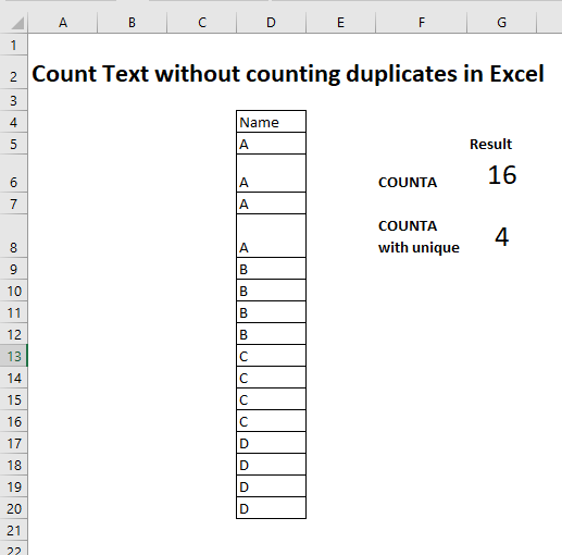
In the example below, we have a list of items with duplicates.

If we use the SUM formula to count the total number of items, there will be duplicates. To exclude the duplicates, you have to follow these steps.

Step 1: Go to cell D1 and enter this formula “=SUMPRODUCT(1/COUNTIF( B1:B11,B1:B11)). B1:B11 is the array range you want to count the total number of unique values in the list.

Step 2: Press enter and the results will be displayed in cell D1. From the displayed results (6) we can see there are no duplicates.

The above formula counts the values of the six items A/B/C/D/E/F.

2. Using a combination of SUM, IF, FREQUENCY, MATCH, and ROW Function

If we want to count unique values that exclude all duplicates (that appear in more than one product), use the combination of these functions.

The sum function allows you to add the values.
For each true condition of IF function, assign value 1.
The FREQUENCY function allows you to count the number of values ignoring texts and zeros. In the first occurrence of the distinct value, it returns an equal number to the number of occurrences of that value. It returns zero for the occurrences that have the same value after the first occurrence.
The MATCH function returns the position of the text value in an array range. The return value acts as the function argument for FREQUENCY.
The ROW function returns the row reference number.

Example: Enter the following formula to count unique values by excluding all duplicates

=SUM(IF(FREQUENCY(MATCH(B1:B11,B1:B11,0),ROW(B1:B11)-ROW(B1)+1)=1,1))

Press enter. The unique value is 3 (Item D/E/F).

3. Using ISNUMBER Function to count numeric numbers

The function we used earlier counts, both texts and numbers, without duplicating. To count only numerals without duplicating, you have to include ISNUMBER function in the formula for finding unique values.

=SUM(IF(ISNUMBER(A2:A10)*COUNTIF(A2:A10,A2:A10)=1,1,0))

Note: Always press Ctrl + Shift + Enter when entering your array formula.

Meanwhile, the lowdown in this function is that it also counts dates and times.

4. Using ISTEXT Function to count text values

You can count the number of texts without duplicating by including the ISTEXT function in the array formula as stated below:

=SUM(IF(ISTEXT(A2:A10)*COUNTIF(A2:A10,A2:A10)=1,1,0))

This formula will display the number of unique texts. It excludes errors, blank cells, logical numbers, numbers, etc.

Always press Ctrl + Shift + Enter when entering your array formula.

5. Using Pivot Table to count text values

Easies way to count the value is by creating the pivot table and using the Count of items

1. Create a pivot table

2. Use Count of Items

3. Output Table

6. Using A Filter

The Filter method is the simplest approach that allows you to remove duplicates and remain with unique values. You can, therefore, use two tricks to get unique values as discussed below.

6.1: Filtering for Unique Values

Steps:

1. Select and make sure the range of cells you want to make unique is in a table.

2. Click on Data then select the Advanced option in the soft & filter group.

3. When the Advanced Filter box pops up, you can filter the range of cells or tables by clicking on the Filer the List, in-place option.

4. You can also copy the result of the filter to another location by clicking on the Copy to another location option.

5. Enter a cell reference in the Copy To box.

6. Alternatively, you can click the Collapse Dialog option to hide the popup window temporarily, select a cell on the worksheet, and then click the Expand option.

7. Finish by checking the Unique Records Only and click OK.

6.2: Removing The Duplicates

The method only affects the values in the range of cells or tables and not values outside. After removing the duplicates, you will keep the first occurrence of the value in the list, while the identical values will be deleted. Therefore, remember to copy the original range of cells to the table to another worksheet before deleting duplicates.

Steps:

1. Start by selecting the active range of cells in a table.

2. Select the Data Tab and click Remove Duplicates in the Data Tools group.

3. You can select one or more columns under the Columns face. Alternatively, you can click Select All to select all columns quickly or Unselect All to clear all columns quickly.

4. Click OK and a message will pop up showing how many duplicates you have removed or how many unique values remain. To dismiss the message, click OK.

5. You can undo the change by clicking Undo or pressing Ctrl + Z

7. Using Amazing Excel Tools

Another simple way to count without duplicates in excel is tools like Kutools by the following steps.

1. Select a blank cell to output the result.

2. Click Kutools>Formula>Helper>Formula Helper.

3. Do the following steps in the formula helper dialog;

Check and select Count unique values in the Choose a formula box. You can check the filter box and type some words to filter the formula names.
Then choose the range in which you want to count unique values in the range box.
Press the OK button.

8. Using A Data Model with A Pivot Table to Count Unique Values

The method applies to newer versions of Microsoft Excel, including Microsoft 365, Excel 2019, Excel 2016, and Excel 2013. To count unique values using this approach, follow these steps:

1. Select any cell in the data and click on the Insert tab in the ribbon.

2. Click on Pivot Table to open a dialogue box.

3. Select the Add this data to the Data Model at the bottom and click OK.

4. In the resulting window, drag the Name column into the Name field and the Profession column or any other in the dataset into the Values field.

5. Click on the small arrow next to the Count of Profession option in the Pivot Table fields.

6. Select the Value Field Settings at the bottom.

7. Finish by selecting the Distinct Count or Unique Count option and click OK.

8. You will have your unique values in the Pivot Table.

9. Using Power Pivot

Power Pivot is also another powerful method you can use to count unique values. However, you will need an enabled Power Pivot tab in your ribbon. That means if your Excel version does not have an already-enabled Power Pivot add-in, you will have to enable it first. Once you have enabled it, you can proceed with the following steps:

1. Go to the Data Model and select the Manage Button.

2. This will open a new blank window if it is your first time importing data.

3. Click on Home Tab and select the “Get External Data” option.

4. You will see various sources and options to upload data. Since you want to upload simple Excel, select the «From Other Sources» option.

5. Scroll down to the end of a new dialogue box opened, select “Excel File”, and click Next.

6. You will need to rename the connection created. For simplicity, you can rename it “Excel”. After that, click on “Browse” to choose an Excel file path.

7. You can click on the “Use the first row as column header” option to make the top column the header. Click on the Next Button to finish.

8. You will see the file imported to the Data Model. Click the Finish button.

9. After importing all the rows successfully, hit the Close Button.

10. With your new worksheet, you will have to create a Pivot Table by clicking on Home and then Pivot Table.

11. Click on the small triangle next to it to expand the columns. That is because you already have the data on the first sheet.

12. After dragging and dropping all the data in their respective fields, you will get a simple Pivot Table.

13. Go back to the Power Pivot window and select the Measure option to create a New Measure.

14. Add your desired description name by typing in the box and the suggestions will pop up automatically. Since you want to count unique values, select the Unique Count function.

15. Press the Tab button or use the bracket to select which column you need the unique count for. For example, if you want the unique count for Profession, your formula will be like this;

=DISTINCTCOUNT (Sheet1[Profession]))

16. Select the Number category since you want to count unique values.

17. Change the format to “Whole Number’ and hit OK to create a new column with unique entries.

I hope this tutorial is comprehensive. Kindly share with friends & thanks for reading!

Источник

Jul

Microsoft Excel provides several functions purposed for counting different kinds of cells, such as blanks or non-blanks, with number, date or text values, containing specific words or character, etc.

In this article, we will focus on the Excel COUNTIF function that is purposed for counting cells with the condition you specify. First, we will briefly cover the syntax and general usage, and then I provide a number of examples and warn about possible quirks when using this function with multiple criteria and specific types of cells.

In essence, COUNTIF formulas are identical in all Excel versions, so you can use the examples from this tutorial in Excel 2016, 2013, 2010 and 2007.

Excel COUNTIF function — syntax and usage
Examples of how to use COUNTIF in Excel
- COUNTIF formula for text and numbers (exact match)
- COUNTIF with wildcard characters (partial match)
- Count if blank or not blank
- Count if greater than, less than or equal to
- COUNTIF formulas for dates
- Excel COUNTIF with multiple criteria
- Count duplicates and unique values
Excel COUNTIF — frequently asked questions and issues

COUNTIF function in Excel — syntax and usage

Excel COUNTIF function is used for counting cells within a specified range that meet a certain criterion, or condition.

For example, you can write a COUNTIF formula to find out how many cells in your worksheet contain a number greater than or less than the number you specify. Another typical use of COUNTIF in Excel is for counting cells with a specific word or starting with a particular letter(s).

The syntax of the COUNTIF function is very simple:

COUNTIF(range, criteria)

As you see, there are only 2 arguments, both of which are required:

range — defines one or several cells to count. You put the range in a formula like you usually do in Excel, e.g. A1:A20.
criteria — defines the condition that tells the function which cells to count. It can be a number, text string, cell reference or expression. For instance, you can use the criteria like these: «10», A2, «>=10», «some text».

And here is the simplest example of Excel COUNTIF function. What you see in the image below is the list of the best tennis players for the last 14 years. The formula =COUNTIF(C2:C15,»Roger Federer») counts how many times Roger Federer’s name is on the list:

Note. A criterion is case insensitive, meaning that if you type «roger federer» as the criteria in the above formula, this will produce the same result.

Excel COUNTIF function examples

As you have just seen, the syntax of the COUNTIF function is very simple. However, it allows for many possible variations of the criteria, including wildcard characters, the values of other cells, and even other Excel functions. This diversity makes the COUNTIF function really powerful and fit for many tasks, as you will see in the examples that follow.

COUNTIF formula for text and numbers (exact match)

In fact, we discussed the COUNTIF function that counts text values matching a specified criterion exactly a moment ago. Let me remind you that formula for cells containing an exact string of text: =COUNTIF(C2:C15,»Roger Federer»). So, you enter:

A range as the first parameter;
A comma as the delimiter;
A word or several words enclosed in quotes as the criteria.

Instead of typing text, you can use a reference to any cell containing that word or words and get absolutely the same results, e.g. =COUNTIF(C1:C9,C7).

Similarly, COUNTIF formulas work for numbers. As shown in the screenshot below, the formula =COUNTIF(D2:D9,5) perfectly counts cells with quantity 5 in Column D.

COUNTIF formulas with wildcard characters (partial match)

In case your Excel data include several variations of the keyword(s) you want to count, then you can use a wildcard character to count all the cells containing a certain word, phrase or letters as part of the cell’s contents.

Suppose, you have a list of tasks assigned to different persons, and you want to know the number of tasks assigned to Danny Brown. Because Danny’s name is written in several different ways, we enter «*Brown*» as the search criteria =COUNTIF(D2:D10, «*Brown*»).

An asterisk (*) is used to find cells with any sequence of leading and trailing characters, as illustrated in the above example. If you need to match any single character, enter a question mark (?) instead, as demonstrated below.

Tip. It is also possible to use wildcards with cell references with the help of the concatenation operator (&). For example, instead of supplying «*Brown*» directly in the formula, you can type it in some cell, say F1, and use the following formula to count cells containing «Brown»: =COUNTIF(D2:D10, «*»&F1&»*»)

Count cells beginning or ending with certain characters

You can use either wildcard character, asterisk (*) or question mark (?), with the criterion depending on which exactly result you want to achieve.

If you want to know the number of cells that start or end with certain text no matter how many other characters a cell contains, use these formulas:

=COUNTIF(C2:C10,»Mr*») — count cells that begin with «Mr».

=COUNTIF(C2:C10,»*ed») — count cells that end with the letters «ed».

The image below demonstrates the second formula in action:

If you are looking for a count of cells that start or end with certain letters and contain the exact number of characters, you use the Excel COUNTIF function with the question mark character (?) in the criteria:

=COUNTIF(D2:D9,»??own») — counts the number of cells ending with the letters «own» and having exactly 5 characters in cells D2 through D9, including spaces.

=COUNTIF(D2:D9,»Mr??????») — counts the number of cells starting with the letters «Mr» and having exactly 8 characters in cells D2 through D9, including spaces.

Tip. To find the number of cells containing an actual question mark or asterisk, type a tilde (~) before the ? or * character in the formula. For example, =COUNTIF(D2:D9,»*~?*») will count all cells containing the question mark in the range D2:D9.

Excel COUNTIF for blank and non-blank cells

These formula examples demonstrate how you can use the COUNTIF function in Excel to count the number of empty or non-empty cells in a specified range.

COUNTIF not blank

In some of other Excel COUNTIF tutorials, you may come across formulas for counting non-blank cells in Excel similar to this one:

COUNTIF(range,»*»)

But the fact is, the above formula counts only cells containing any text values, meaning that cells with dates and numbers will be treated as blank cells and not included in the count!

If you need a universal COUNTIF formula for counting all non-blank cells in a specified range, here you go:

COUNTIF(range,»<>»)

COUNTIF(range,»<>»&»»)

This formula works correctly with all value types — text, dates and numbers — as you can see in the screenshot below.

COUNTIF blank

If you want the opposite, i.e. count blank cells in a certain range, you should adhere to the same approach — use a formula with a wildcard character for text values and with the «» criteria to count all empty cells.

Formula to count cells not containing any text:

COUNTIF(range,»<>»&»*»)

Since an asterisk (*) matches any sequence of text characters, the formula counts cells not equal to *, i.e. not containing any text in the specified range.

Universal COUNTIF formula for blanks (all value types):

COUNTIF(range,»»)

The above formula correctly handles numbers, dates and text values. For example, here’s how you can get the number of empty cells in the range C2:C11:

=COUNTIF(C2:C11,»»)

Please be aware that Microsoft Excel has another function for counting blank cells, COUNTBLANK. For instance, the following formulas will produce exactly the same results as the COUNTIF formulas you see in the screenshot above:

Count blanks: =COUNTBLANK(C2:C11)

Count non-blanks: =ROWS(C2:C11)*COLUMNS(C2:C11)-COUNTBLANK(C2:C11)

Also, please keep in mind that both COUNTIF and COUNTBLANK count cells with empty strings that only look blank. If you do not want to treat such cells as blanks, use this formula instead:

=ROWS(C2:C11)*COLUMNS(C2:C11)-COUNTIF(C2:C11,»<>»&»»)

For more information about counting blanks and not blanks in Excel, please see:

3 ways to count empty cells in Excel
How to count non-empty cells in Excel

COUNTIF greater than, less than or equal to

To count cells with values greater than, less than or equal to the number you specify, you simply add a corresponding operator to the criteria, as shown in the table below.

Please pay attention that in COUNTIF formulas, an operator with a number are always enclosed in quotes.

CriteriaFormula ExampleDescriptionCount if greater than=COUNTIF(A2:A10,»>5″)Count cells where value is greater than 5.Count if less than=COUNTIF(A2:A10,»<5″)Count cells with values less than 5.Count if equal to=COUNTIF(A2:A10,»=5″)Count cells where value is equal to 5.Count if not equal to=COUNTIF(A2:A10,»<>5″)Count cells where value is not equal to 5.Count if greater than or equal to=COUNTIF(C2:C8,»>=5″)Count cells where value is greater than or equal to 5.Count if less than or equal to=COUNTIF(C2:C8,»<=5″)Count cells where value is less than or equal to 5.

You can also use all of the above formulas to count cells based on another cell value, you will just need to replace the number in the criteria with a cell reference.

Note. In case of a cell reference, you have to enclose the operator in quotes and add an ampersand (&) before the cell reference. For example, to count cells in the range D2:D9 with values greater than a value in cell D3, you use this formula =COUNTIF(D2:D9,»>»&D3):

If you want to count cells that contain an actual operator as part of the cell’s contents, i.e. the characters «>», «<» or «=», then use a wildcard character with the operator in the criteria. Such criteria will be treated as a text string rather than a numeric expression. For example, the formula =COUNTIF(D2:D9,»*>5*») will count all cells in the range D2:D9 with contents like this «Delivery >5 days» or «>5 available».

Using Excel COUNTIF function with dates

If you want to count cells with dates that are greater than, less than or equal to the date you specify or date in another cell, you proceed in the already familiar way using formulas similar to the ones we discussed a moment ago. All of the above formulas work for dates as well as for numbers. Let me give you just a few examples:

CriteriaFormula ExampleDescriptionCount dates equal to the specified date.=COUNTIF(B2:B10,»6/1/2014″)Counts the number of cells in the range B2:B10 with the date 1-Jun-2014.Count dates greater than or equal to another date.=COUNTIF(B2:B10,»>=6/1/2014″)Count the number of cells in the range B2:B10 with a date greater than or equal to 6/1/2014.Count dates greater than or equal to a date in another cell, minus x days.=COUNTIF(B2:B10,»>=»&B2-«7»)Count the number of cells in the range B2:B10 with a date greater than or equal to the date in B2 minus 7 days.

Apart from these common usages, you can utilize the COUNTIF function in conjunction with specific Excel Date and Time functions such as TODAY() to count cells based on the current date.

CriteriaFormula ExampleCount dates equal to the current date.=COUNTIF(A2:A10,TODAY())Count dates prior to the current date, i.e. less than today.=COUNTIF(A2:A10,»<«&TODAY())Count dates after the current date, i.e. greater than today.=COUNTIF(A2:A10,»>»&TODAY())Count dates that are due in a week.=COUNTIF(A2:A10,»=»&TODAY()+7)Count dates in a specific date range.=COUNTIF(B2:B10, «>=6/1/2014»)-COUNTIF(B2:B10, «>6/7/2014»)

Here is an example of using such formulas on real data (at the moment of writing today was 25-Jun-2014):

Excel COUNTIF with multiple criteria

In fact, Excel COUNTIF function is not exactly designed to count cells with multiple criteria. In most cases, you’d use its plural counterpart, the COUNTIFS function to count cells that match two or more criteria (AND logic). However, some tasks can be solved by combining two or more COUNTIF functions in one formula.

COUNTIF — COUNTIF to count numbers within a range

One of the most common applications of Excel COUNTIF function with 2 criteria is counting numbers within a specific range, i.e. less than X but greater than Y. For example, you can use the following formula to count cells in the range B2:B9 where a value is greater than 5 and less than 15.

=COUNTIF(B2:B9,»>5″)-COUNTIF(B2:B9,»>=15″)

COUNTIF + COUNTIF to count cells with multiple OR criteria

In situations when you want to get several different items in a range, add 2 or more COUNTIF functions together. Supposing, you have a shopping list and you want to find out how many soft drinks are included. To have it done, use a formula similar to this:

=COUNTIF(B2:B13,»Lemonade»)+COUNTIF(B2:B13,»*juice»)

Please pay attention that we’ve included the wildcard character (*) in the second criterion, it is used to count all kinds of juice on the list.

In the same manner, you can write a COUNTIF formula with several conditions. Here is an example of the COUNTIF formula with multiple OR conditions that counts lemonade, juice and ice cream:

=COUNTIF(B2:B13,»Lemonade») + COUNTIF(B2:B13,»*juice») + COUNTIF(B2:B13,»Ice cream»)

For other ways to count cells with OR logic, please see this tutorial: Excel COUNTIF and COUNTIFS with OR conditions.

Using COUNTIF function to find duplicates and unique values

Another possible usage of the COUNTIF function in Excel is for finding duplicates in one column, between two columns, or in a row.

Example 1. Find and count duplicates in 1 column

For example, this simple formula =COUNTIF(B2:B10,B2)>1 will spot all duplicate entries in the range B2:B10 while another function =COUNTIF(B2:B10,TRUE) will tell you how many dupes are there:

Example 2. Count duplicates between two columns

If you have two separate lists, say lists of names in columns B and C, and you want to know how many names appear in both columns, you can use Excel COUNTIF in combination with the SUMPRODUCT function to count duplicates:

=SUMPRODUCT((COUNTIF(B2:B1000,C2:C1000)>0)*(C2:C1000<>»»))

We can even take a step further and count how many unique names there are in Column C, i.e. names that do NOT appear in Column B:

=SUMPRODUCT((COUNTIF(B2:B1000,C2:C1000)=0)*(C2:C1000<>»»))

Tip. If you want to highlight duplicate cells or entire rows containing duplicate entries, you can create conditional formatting rules based on the COUNTIF formulas, as demonstrated in this tutorial — Excel conditional formatting formulas to highlight duplicates.

Example 3. Count duplicates and unique values in a row

If you want to count duplicates or unique values in a certain row rather than a column, use one of the below formulas. These formulas might be helpful, say, to analyze the lottery draw history.

Count duplicates in a row:

=SUMPRODUCT((COUNTIF(A2:I2,A2:I2)>1)*(A2:I2<>»»))

Count unique values in a row:

=SUMPRODUCT((COUNTIF(A2:I2,A2:I2)=1)*(A2:I2<>»»))

Excel COUNTIF — frequently asked questions and issues

I hope these examples have helped you to get a feel for the Excel COUNTIF function. If you’ve tried any of the above formulas on your data and were not able to get them to work or are having a problem with the formula you created, please look through the following 5 most common issues. There is a good chance that you will find the answer or a helpful tip there.

1. COUNTIF on a non-contiguous range of cells

Question: How can I use COUNTIF in Excel on a non-contiguous range or a selection of cells?

Answer: Excel COUNTIF does not work on non-adjacent ranges, nor does its syntax allow specifying several individual cells as the first parameter. Instead, you can use a combination of several COUNTIF functions:

Wrong: =COUNTIF(A2,B3,C4,»>0″)

Right: =COUNTIF(A2,»>0″) + COUNTIF(B3,»>0″) + COUNTIF(C4,»>0″)

An alternative way is using the INDIRECT function to create an array of ranges. For example, both of the below formulas produce the same result you see in the screenshot:

=SUM(COUNTIF(INDIRECT({«B2:B8″,»D2:C8″}),»=0»))

=COUNTIF($B2:$B8,0) + COUNTIF($C2:$C8,0)

2. Ampersand and quotes in COUNTIF formulas

Question: When do I need to use an ampersand in a COUNTIF formula?

Answer: It is probably the trickiest part of the COUNTIF function, which I personally find very confusing. Though if you give it some thought, you’ll see the reasoning behind it — an ampersand and quotes are needed to construct a text string for the argument. So, you can adhere to these rules:

If you use a number or a cell reference in the exact match criteria, you need neither ampersand nor quotes. For example:

=COUNTIF(A1:A10,10)
or
=COUNTIF(A1:A10,C1)

If your criteria includes text, wildcard character or logical operator with a number, enclose it in quotes. For example:

=COUNTIF(A2:A10,»lemons»)
or
=COUNTIF(A2:A10,»*») or =COUNTIF(A2:A10,»>5″)

In case your criteria is an expression with a cell reference or another Excel function, you have to use the quotes («») to start a text string and ampersand (&) to concatenate and finish the string off. For example:

=COUNTIF(A2:A10,»>»&D2)
or
=COUNTIF(A2:A10,»<=»&TODAY())

If you are in doubt whether an ampersand is needed or not, try out both ways. In most cases an ampersand works just fine, e.g. both of the below formulas work equally well.

=COUNTIF(C2:C8,»<=5″)
and
=COUNTIF(C2:C8,»<=»&5)

3. COUNTIF for formatted (color coded) cells

Question: How do I count cells by fill or font color rather than by values?

Answer: Regrettably, the syntax of the Excel COUNTIF function does not allow using formats as the condition. The only possible way to count or sum cells based on their color is using a macro, or more precisely an Excel User-Defined function. You can find the code working for cells colored manually as well as for conditionally formatted cells in this article — How to count, sum and filter cells by color in Excel.

4. #NAME? error in the COUNTIF formula

Issue: My COUNTIF formula throws a #NAME? error. How can I get it fixed?

Answer: Most likely, you have supplied an incorrect range to the formula. Please check out point 1 above.

5. Excel COUNTIF formula not working

Issue: My COUNTIF formula is not working! What have I done wrong?

Answer: If you have written a formula which is seemingly correct but it does not work or produces a wrong result, start by checking the most obvious things such as a range, conditions, cell references, use of ampersand and quotes.

Be very careful with using spaces in a COUNTIF formula. When creating one of the formulas for this article I was on the verge of pulling my hair out because the correct formula (I knew with certainty it was right!) wouldn’t work. As it turned out, the problem was in a measly space somewhere in between, argh… For instance, look at this formula:

=COUNTIF(B2:B13,» Lemonade»).

At first sight, there is nothing wrong about it, except for an extra space after the opening quotation mark. Microsoft Excel will swallow the formula just fine without an error message, warning or any other indication, assuming you really want to count cells containing the word ‘Lemonade’ and a leading space.

If you use the COUNTIF function with multiple criteria, split the formula into several pieces and verify each function individually.

And this is all for today. In the next article, we will explore several ways to count cells in Excel with multiple conditions. Hope to see you next week and thanks for reading!

You may also be interested in

Count cells in Excel: COUNT and COUNTA functions with formula examples
Count distinct and unique values in Excel
Count characters in Excel: total or only specific characters in a cell / range

Excel: featured articles

Merge multiple sheets intoone
Combine Excel files into one
Compare two files / worksheets
Merge 2 columns in Excel
Compare 2 columns in Excel for matches and differences
How to merge two or more tables in Excel
CONCATENATE in Excel: combine text strings, cells and columns
Create calendar in Excel (drop-down and printable)
3 ways to remove spaces between words in Excel cells

Older Comments

Newer Comments

renjith says:

December 9, 2016 at 10:13 am

i have data of 500 employee ID’s with different tasks. I want to use the function countif to get the no of tasks per employee id in mass, it is possible please help me

Reply
Nitin says:

December 9, 2016 at 8:16 am

Please help me i want to calculate electricity rate in excel
Example:
Sr. No House no Name Meter reading
1 1 ABC 50
2 2 XYZ 56
Criteria is if reading 0 to 50 then 0 rs charges if reading >50 but 100 but 150 then 4 rs charges.

Reply
Azam says:

December 3, 2016 at 2:04 pm

Qty. Rate
2 699
1 899
1 809
2 539
1 719
1 539
3 685
1 539

More then 599 and lees or equal to 799
I require output : 6
Detail .
(699 -> 2)+(719 -> 1) +(685 -> 3) = 6

Reply
Azam says:

December 3, 2016 at 2:03 pm

Qty. Rate
2 699
1 899
1 809
2 539
1 719
1 539
3 685
1 539

I use
=COUNTIFS(A:A,»>599″,A:A,» 2)+(719 -> 1) +(685 -> 3) = 6

Reply
Gavin says:

November 30, 2016 at 9:59 am

hi i was wondering if you can use the countif function with a cell reference as part of the criteria. basically instead of saying =countif(Range,»<5″) rather saying =countif(range,»<A7″). your help would be greatly appreciated.

thanks
Gavin

Reply
Parminder says:

November 7, 2016 at 8:38 am

A B C D E F G H I J
B 1 0 1 1 1 0 1 1 1
C 0 1 0 0 0 1 0 0 0
D 0 0 1 1 0 0 1 0 1
E 1 1 1 0 1 1 0 1 0
F 0 1 0 1 0 0 1 0 1
G 0 0 1 0 0 1 0 0 0
H 1 0 0 1 1 0 1 1 1
I 0 1 1 0 0 0 0 0 1
J 1 0 1 1 1 1 1 1 0

find duplicate column..
highlight it

Help me with this…

Reply
- Parminder says:
  
  December 6, 2016 at 9:48 am
  
  can anyone help me with this ??
  
  i can find the duplicates column in alphabetic mode but i can’t in numeric mode
  
  please help me out with this
  
  Reply
Khamkeo says:

October 26, 2016 at 4:37 pm

What about count if greater than 5 and less than 8 for example? or between something?

Reply
- Svetlana Cheusheva (Ablebits Team) says:
  
  October 27, 2016 at 8:37 am
  
  Hi Khamkeo,
  
  In this case, you need to use the COUNTIFS function, for example:
  
  =COUNTIFS(A2:A10,»>5″, A2:A10,»<8″)
  
  Reply
Traian says:

October 23, 2016 at 11:30 am

i need help: I have a leads excel (clients) and i plan to calculate how many leads we got:
-yesterday
-today
-last7days
-this month
I have P column that have «7» standard possible answers; like the state of the lead. I need a formula for each state of the lead to count the nr of leads for the above time periods.

Thanks,
I really appreciate this answer i tried for one week to do it.

Reply
Usman says:

October 20, 2016 at 2:10 pm

Hi,
I need help, if I have same words from sheet 1, and i want to count the words in 6 rows in sheet 2. how?
e.g.
sheet 1 — ABC (AE1) criteria
Sheet 2 — A1-F1 range
By using countif formula.

once i put the this formula:COUNIF(‘Sheet1’!AE1,»*ABC*»)

but it is calculating multiple.

Reply
Jenna says:

October 20, 2016 at 3:18 am

Hi, I am having a problem counting how many part numbers with shortages on a multiple data. See below data:

YV756A YV756B YV441G YT081A YT081B
4100023-003 -1 0 -1 -1 -1
4100024-001 0 0 0 0 -1
4100142-001 -1 -1 -1 -1 -1

Need to count how many part number with shortage on following models:
YV756 =
YV441 =
YT081 =

this is considering if YV756A and YV756B has -1 on each, it will take only as 1 part number with shortage.

Please help me create formula to count this.

thanks a lot!
Jenna

Reply
GREG says:

October 19, 2016 at 7:59 am

I WANT TO COUNT WITH IF BUT AT NEGATIVE
EXMPL
SUMIF -> IF ISNT «THIS»
?

Reply
- Svetlana Cheusheva (Ablebits Team) says:
  
  October 19, 2016 at 9:39 am
  
  Hi Greg,
  
  You can use the «not equal to» operator (<>) e.g.:
  
  =COUNTIF(A1:A10, «<>»&5)
  
  =COUNTIF(A1:A10, «<>»&»text»)
  
  Reply
Krishna says:

October 19, 2016 at 4:56 am

Sir
COUNTIF(G7:G315,»SC») is 38
and I want to count How many R is entered in the next column exact SC means in column H7:H315. pl do the needful and Give formula

Reply
JMK says:

October 18, 2016 at 6:52 pm

I need help counting unique invoices touched by the collector per work day. I used If(I1=I2,0,1) but still getting some duplicate invoices for others. I need column I to give the count of unique invoices touched that day.
Thanks,
JM

Reply
- Svetlana Cheusheva (Ablebits Team) says:
  
  October 19, 2016 at 9:51 am
  
  Hello!
  
  Please check out the following tutorial, hopefully you will find a proper formula for your task there:
  How to count distinct and unique values in Excel
  
  Reply
Reshma says:

October 17, 2016 at 7:37 am

I need a formula to get the total count of non empty columns in excel which is having «n» number of columns.

Reply
Dominy says:

October 14, 2016 at 5:05 pm

Ok I have bee through a few help forums now and got tired of searching. I was trying to utilize a Countifs formula to determine employees available to work during certain time frames. Due to the way our system exports the information, an excel formula would work best. Here is how info is exported to excel:
A B C D E F
Name From To Sun Mon Tue
Employee 13:00 00:00 TRUE TRUE FALSE

What I need to do is count how many employees are available during certain times each day, example:
Time Sun Mon Tue
1pm-7pm 1 1 0

Any assistance would be greatly appreciated cause this type of formula is not my strong suit.

Reply
Manssor says:

October 12, 2016 at 7:54 am

Thank you for the simple clear detailed information.
You are an angel.

Reply
Denis says:

October 11, 2016 at 1:54 pm

Hi, how do I count the number of cells in a range that are bigger than 0?
The numbers in the cells are the results of formulas though.
Thanks for your help.

Reply
Stella M says:

September 30, 2016 at 1:53 pm

Hi there,

I have a complex spreadsheet and I want to have a formula calculating the following:
From a range of cells to take a particular value (name) and then from another range of cells (column) to take another value matching the row with the name, then to count the matches in the cell.
I have tried this formula
=IF(AND(‘Domain 1′!E6=»Andrea»,’Domain 1’!Q6=»Food»),1,0)

but the thing is that I need the formula to look at a range of cells in two different columns and then to sum up these values.

I would really appreciate if you can help me

Reply
Shivani says:

September 29, 2016 at 8:18 pm

Hi, I have a spreadsheet for analysing exam results. I need to count and summarise each student’s results against each course, e.g. for each student, indicate:
pass (where all 4 subjects passed)

or fail in maths, fail in english (the rest are pass so silent).

or
CNC (where absent)

So how do I insert the text depending on pass or fail per subject.

Thanks.

Reply
Naveed Khalil says:

September 23, 2016 at 9:48 am

Hi,,You are doing best.
I need help.
in column A, i will enter the due date, e.g. due date is 15/09/2016. now i want that if the due date expires and extends to 19/09/2016 then fine of Hundred dollar per day comes automatically in column B and for 19/09/2016 fine will be 400.
Your nice help will be appreciated.
reply should be on email.
Thanks

Reply
Tiffany says:

September 21, 2016 at 5:25 pm

Hello,

I have a list of departments that I am trying to find <=2.0 hours for each department from a pivot table list of employees. I cannot figure out the best way to use the countif function to find only that department name and how many times that department comes up with less than or equal to 2 hours.

Column A: Employee Name
Column B: Department They Work In ex. Pack Room
Column C: Total number of hours worked

I need the Countif function to know to only look up the Pack Room Hours in column B and only count hours that are <=2.0.

I’ve tried using DCount but still can’t get my result.

Reply
Kristiane Esporas says:

September 18, 2016 at 2:28 pm

Hi Svetlana,

Thank you for this very helpful article. I’m trying to use the countifs function, however it’s not working for me. Here’s the scenario.

I have one question which shows a list of anawer.

Ex: How likely will you buy this?
Product 1, Produt 2, Product 3
In each cell there’s a drop down list of the answers such as 3- will buy it, 2-somehow will buy it ans 1-not going to buy it.

I’m using =countifs(A2:A102,»3″, A2:A102,»2″, A2:A102, «1»)

but it’s not even counting

Hope you could help with this.

Thanks a lot!

Reply
- Svetlana Cheusheva (Ablebits Team) says:
  
  September 19, 2016 at 8:39 am
  
  Hi Kristiane,
  
  First off, remove double quotes surrounding numbers because they turn numbers into text strings.
  
  If you need to get the total count of answers 1, 2 and 3, then add up 3 different COUNTIF functions, because COUNTIFS works with the AND logic while you need OR:
  =countif(A2:A102,3) + countif(A2:A102, 2) + countif(A2:A102,1)
  
  If you want the individual count for each type of answers, then use 3 separate formulas like this: =countif(A2:A102,3)
  
  Reply
Rakesh says:

September 16, 2016 at 8:54 am

hi
i want to know the formula which can give me best answer

example-

30 qty pack is equal to 1 duty

he pack 35 then also 1 duty

he pack 25 then also 1 duty

if he pack 60 then will be 2 duties

Reply
Christine says:

September 15, 2016 at 5:26 pm

Hello:
I am trying to count blank cells within a range (rows). I’m only interested if there are 3 or more blank cells beside each other. If cells A1 and B1 are blank and C1 is not blank, I don’t need to know about cells A1 and B1. However if cells A1, B1, C1 are blank, then I want to know. In addition, if there are subsequent series of blank cells, for example M1, N1, O1, P1, I also want to know.

Is there a way to do this?
Thanks!
Christine.

Reply
Anupam says:

September 2, 2016 at 4:41 am

Hi,

I want to use the countif formula for the list of the descriptions (in one column). In these descriptions, there are many cells with more than 255 characters. How to use countif here. I am getting the answers for all the description cells wherever the character length is less than 255. For others, » #value! «.

Can you please help me?
Also, I want to use vlookup for these description columns. How to do that?

Reply
Kayla Kedel says:

September 1, 2016 at 9:29 pm

Hi!

I have a spreadsheet with employees, hire dates, managers, department. I have a second tab that keeps count by all employees, then broken down by each company and department.. I cannot figure out how to group the hire date and department to automatically count for me when I add a new person. we are about to hire 200+ so having it automatically update would be so much help. can you help me figure out what I need to put in the date part and how do I group hire date (ex. Jun-16) and department (ex. Maintenance) to make my formula work?

Reply
nats says:

September 1, 2016 at 3:22 am

hi, please help… i need to have a formula that will count entries in the specified range, with two conditions. ive tried this but it doesn’t work

=COUNTIFS(D13:Q13,»C», D13:Q13,»X»)

I really need help on this, thanks and God bless

Reply
Rich says:

August 26, 2016 at 10:36 am

Hi,

I am using this formula

=IF(COUNTIFS($B$3:$B$1100:$G10:$G$1100,B10,$B$3:$B$1100:$G10:$G$1100,G10)>1,»FT»,»PT»)

I have two colums AM and PM, I am trying to use this to highlight the duplicate number for a person i.e if the persons number shows up in AM an PM it will show FT and if it shows in AM but PM is blank will show PT. — This formula works but the problem Im having is when both Am and PM show «0» or are blank the formula still gives me FT when I need it to stay blank.

Can you help?

Reply
jim says:

August 25, 2016 at 12:27 pm

please help need to find a way to to count how many times a person was late,i.e. d2:d25 =paul,e2:e25 =are times started ie 10:00,10:15 ect.start time is 10:00. i use this,COUNTIF(e2:e25″>10:00″)for the total count,but i need to find a way
to count for each employee thank you

Reply
- Svetlana Cheusheva (Ablebits Team) says:
  
  August 25, 2016 at 3:52 pm
  
  Hi Jum,
  
  You can use COUNTIFS to count with multiple criteria:
  
  =COUNTIFS(E2:E25, «>10:00», D2:D25, «paul»)
  
  Reply
sz says:

August 25, 2016 at 10:12 am

How to count duplicates of 2nd column based on 1st column in a large excel file. Eg :

1 a
1 b
2 a
2 a
2 d
2 c
2 c
4 e

Output Required :
1 a 1 [ Count of «a» in «1» : One Time ]
1 b 1
2 a 2
2 c 2 [ Count of «c» in «2» : Two Time ]
2 d 1
4 e 1

Reply
Per says:

August 22, 2016 at 11:51 am

Hello! What a great post.

I have some trouble counting a specific value in excel. I have a cell that I want to count the amount of cells from a row that contains the specific value «em». So far so good, but there is a catch. I only want it to count it as 1 if the cells with «em» comes after each other. Meaning if it finds three cells in a row like this: «em» «em» «em» «sm», it should only count it as 1. And: «em» «em» «sm» «em» «em» as two.

Hope you understood the question, and thanks a lot for any help!

Reply
Andrea says:

August 18, 2016 at 1:19 pm

Hello…

Do you know if this is possible ?
I have a workbook. One workbook per Month. Each workbook will have 1 worksheet per day (so between 29 and 31 sheets per workbook)

(In this example I have August 1 — August 4 and a Summary Sheet)

I need a formula that will Find a name (In this case I used Captain1 or FF1 etc. instead of actual names) and find what is in the time Off column and total it on the Summary sheet.

I want the summary sheet to populate as new sheets are created. Is there a way to write a formula telling Excel to look in ANY and ALL sheets in the entire workbook and total those form me??

I can’t figure out how to do it as technically the sheets haven’t been created yet…..

Reply
Michael Mwenda says:

August 16, 2016 at 1:49 pm

hi
I wanted to enter these values 2724742560in a cell of a spreadsheet but after pressing the enter key the cell displayed #########. please explain why and how could I rectify the situation.

Reply
- Svetlana Cheusheva (Ablebits Team) says:
  
  August 17, 2016 at 10:16 am
  
  Hi Michael,
  
  Most likely the cell is not wide enough to display the value, so just make it a bit wider. To quickly change the column width to fit the contents, select the column, and double-click the boundary to the right of the selected column heading.
  
  Reply
Michael Mwenda says:

August 16, 2016 at 1:39 pm

state the results of the function,=IF(COUNT IF(B2:B9,»>65″)>5,»YES»,»NO»)

Reply
- Svetlana Cheusheva (Ablebits Team) says:
  
  August 17, 2016 at 10:23 am
  
  Michael,
  
  If the range B2:B9 contains more than 5 cells with values greater than 65, return YES, otherwise NO.
  
  BTW, COUNTIF should be spelled with no space in between like this:
  =IF(COUNTIF(B2:B9,»>65″)>5,»YES»,»NO»)
  
  Reply
Carl says:

August 11, 2016 at 10:17 pm

Hi,

Using Excel 2013. I want to return the count of the number of cells that are colored a specific color AND have a specific value.
FOR EXAMPLE: I have APPLES (red), GRAPES (green) and STRAWBERRIES (red). I want to only return the number of red apples, not everything red. Can I do this? Please help
P.S. I am not using COUNTIF to count apples only as I am using that formula to return that value in a different cell.

Reply
Somasundaram says:

August 10, 2016 at 1:08 pm

Hello,

I want to count the Entry in excel what are entries are entered as well as i have to sum the pages in pages column.

for example

Name Pages Stage
1234_AAA 100 Stage1
1345_AAA 200 Stage2
1234_AAA 300 Stage1
1568_BBB 400 Stage3
1345_AAA 500 Start2

I need below output automatically

Count Total Pages
1234_AAA 2 400
1345_AAA 2 700
1568_BBB 1 400

Stage wise total pages
Stage 1 Stage 2 Stage 3
1234_AAA 2
1345_AAA 2
1568_BBB 1

Reply
Maria says:

August 3, 2016 at 7:27 pm

Hello,

Can you break this formula down for me?

COUNTIF9G31:BC31,»*x*»)/2

Thank you.

Reply
Ester says:

August 3, 2016 at 9:33 am

Hi Svetlana,
I’m trying to count the blank cells in a column after a specific date. For example, I have a list with several projects I need to close before 31/03/2017. I’ve foreseen a column with the date of closure and I can count the project that I’ve closed allready and those I’ve closed to late: =COUNTIF(P2:P33;»>31/03/2017″) but when the project stays open, and the cell is empty, I can’t count those. I’m looking for a formula that can count the projects that have passed 31/03/2017.
Can you help me?
Thank you

Reply
Sanjeet Shokeen says:

July 30, 2016 at 10:48 am

I have a table in which first column i add date 1 July to 26 July 2016. In second column, I give rating to me (e.g. 0 to 10). I want to sum my rating only past 5 days but when last 5 day rating is less than 2, then add one more day. e.g.
Date Rating
15 July 5
16 July 3
17 July 0
18 July 8
19 July 2
20 July 6
21 July 7
23 July 1
24 July 5
25 July 6
26 July 3

when I sum last 5 day (21 July to 26 July) is 22, but 23 July my rating is less than 2 than I add one more day in rating (20 July to 26 July) than my rating is 27, I remove 23 July in my life.

Can you you help me in this.

Than You.

Reply
- sanjeet shokeen says:
  
  August 6, 2016 at 8:45 am
  
  any one can help me in this.
  
  Reply
Cmcd says:

July 28, 2016 at 11:25 pm

I want to count when a range of cells (m8:m17) are not equal to 0 but only when cell m6 isn’t 0.
Is this possible?

Reply
- Svetlana Cheusheva (Ablebits Team) says:
  
  July 29, 2016 at 8:49 am
  
  Hi!
  
  The following formula counts how many cells in the range M8:M17 are not equal to 0 when M6 is not equal to zero, and returns an empty string (blank cell) otherwise:
  =IF(M6<>0, COUNTIF(M8:M17,»<>»&0), «»)
  
  If you are looking for something different, please clarify.
  
  Reply
Shahrul says:

July 13, 2016 at 11:31 am

Hi, I would like to count how many rows (in total) that fulfil more than 2 criterias. For each row, there is a unique ID. For example, one unique ID has 5 rows of Product A and 3 rows of Product B. Under Product A and B, the unique ID has different amount.

The criteria is Product A has amount more and equal to 1,000. Product B has amount more and equal to 1,000.

My question is what formula to use to calculate how many rows (in total) that this unique ID has and it need to fulfil the 2 criterias.

Appreciate your assistance on this.

Thank you.
Shahrul

Reply
joanna says:

July 12, 2016 at 8:05 am

sheet1 i have item and quantity then i want to transfer the value of all items that has >=1 to sheet2? how can i do that?? thank you

Reply
Sydney says:

July 9, 2016 at 10:52 pm

Please help me to come up with a formula used to show exact date in which data was entered in a cell.

Reply
- Svetlana Cheusheva (Ablebits Team) says:
  
  July 11, 2016 at 9:14 am
  
  Hello Sydney,
  
  Please check out the following example:
  
  How to insert today date & current time as unchangeable time stamp
  
  Reply
Ross says:

July 5, 2016 at 4:18 pm

Hi, I am trying to evaluate the results of suppliers / products against specifications. In particular I am wanting to calculate the % of intakes from a particular item that meet a specification. e.g.;

SUPPLIER PRODUCT Spec No. in spec % meeting spec
Joe blogs Apples 0.10 50 98

For the ‘No. in spec result’ I am using a COUNTIFS formula where ‘criteria 1’ is the spec value inputted another cell («<=»&C2). This seems to work fine where the there is a value in the ‘spec’ cell, but for some products there isn’t a spec so I enter N/A. In such instances the COUNTIFS formula returns a seemingly random numeric figure, instead of an error. This in turn returns a false value in the % meeting spec column… Please can anyone help?

Reply
Amanda says:

July 5, 2016 at 2:58 pm

I have a mixed text and number format array that I am trying to use multiple conditions to count items. Columns are numbered for course rotations 1-13. rows are random and not important. Individual cells contain student name, rotation name and MAY contain which weeks withing a 4 week rotation they will be there. Eg one cell may have Smith GI which corresponds to a student for all 4 weeks and another have Green GI (1,2) meaning they are there only 2 weeks. I am trying to get the output in number of students per week per rotation. for the above would be 2,2,1,1. Goal would be to express results in an array of rows by rotation#/week and columns by rotation name. Tried using multiple countif functions as follows: =COUNTIFS($C$2:$C$18,»*GI*»&»*weeks*»&»*1*») + COUNTIFS($C$2:$C$18,»*GI*»,$C$2:$C$18,»weeks») but didn’t work. Also figure there should be an easier way to use a reference cell for the rotations text (GI) and the week (for the above formula used week 1) Any suggestions? Thanks in advance!!!

Reply
jen says:

June 30, 2016 at 8:35 pm

column A column B
1200018401 9000035943
1200018402 9000035944
1200018392 blank
1200018393 blank
1200018396 blank
1200018397 blank

How can I calculate whenever column A has a number and column B has a blank. I need to know that total blank number

Reply
- Vijaykumar Shetye says:
  
  July 28, 2016 at 9:19 pm
  
  Dear Jen,
  
  Use the formula
  =COUNTIFS(A1:A100,»>»&0,B1:B100,»»)
  
  Change the range of the cells as required.
  Do let me know if this is what you wanted to do.
  
  Regards
  
  Vijaykumar Shetye, Goa, India
  
  Reply
jen says:

June 30, 2016 at 8:32 pm

Im trying to count blank cells. I have column A with numbers in it and column B with both numbers and blanks. What I need to know is how to count column A with numbers with Column B to get only the total number of blanks

Reply
Amjad says:

June 28, 2016 at 12:28 pm

i want to count 2 values in one cell from different column

ex. count A for me from one column (means column A) and < 5 from another column (means column B)in one cell.
what will be the formula
thanks

Reply
Matt says:

June 10, 2016 at 12:07 pm

I’m trying to use the COUNTIF function to count cells in a column that are >0, but I don’t want it to include hidden cells. How do I select an entire column as my range, but not include hidden cells in my count?

Reply
- Matt says:
  
  June 10, 2016 at 12:15 pm
  
  Here is the formula that I tried using =COUNTIF(Compile!N:N,»>0″)
  
  Reply
Gary says:

June 8, 2016 at 9:16 pm

What do I do if I want to refer to a text cell to find values in a range?

For example, I have a table with service time. The header for columns will have text for «10-14» or «15-19″, etc. I want to use the header text as a variable for my criteria, kind of like =Countif($B$2:$B$2000,»>=»&Value(Left(Header,2)),$B$2:$B$2000,»<=»&Value(Right(Header,2)))

(the above does not work, wondering if I need an Indirect() function in there somewhere…?

Reply
Elaine says:

June 7, 2016 at 2:28 pm

Hi I have a question:
I have a list of values in Column A on tab 1 — Product
potato
tomato
squash
corn etc and they are unique

On the tab 2 I have 2 columns:
Column A has the same values as column A on tab 1 but they could repeat, and column B has some text, for example color. Not all column B is populated
potato brown
tomato red
potato purple
squash
corn yellow

I need to calc. value in col B on tab A, where it will count for each of the col A entries on tab A it will count how many have values on tab 2
So it will be on tab A
Potato 2
tomato 1
squash 0
corn 1

Thank you!

Reply
Manish Gupta says:

May 28, 2016 at 2:31 pm

In column «S», I have numbers 1,2,3… (based on the formula that checks a value in Column A (if blank, gives blank… else a number in Ascending Order).
I have a similar value in Column X as well. 1,2,3,… etc.
in between, I have Certain values in Columns U & V (derived from certain formula). In column Y3 I am trying to calculate using the below formula…

=COUNTIFS(S:S,»<«&X3,V:V,U3)
but I am getting everything as ‘0’.

Please advice.

thanks,

Manish Gupta

Reply
sonam says:

May 27, 2016 at 12:08 am

=COUNTIF($D$9:$D$38,»B»)+COUNTIF($J$9:$J$38,»>=16″)

with the above formula,I wanted to find out total numbers of boys passed and failed in three subjects,English,Maths,and science.Full mark is 40 and pass mark is 16

this is my table

sl Name gender english maths science
1 Sunny M 22 21 18
2 mike F 14 12 19
3 Bunny M 22 21 18
4 mike F 14 12 19

so I wanted to find out total boys and girls failed and passed using the formula

Reply
Jeff H says:

May 19, 2016 at 5:53 pm

I have been reading up on this but have been unsuccessful in assembling a working formula to solve my issue.

I am downloading a YTD sales report weekly and need to report out some key KPI’s.

The goal is to dump the sales report YTD extract into the model weekly and have all the KPI’s update based on date ranges, dsum logic, etc.

I need to calculate the # of orders and the # of shipments (referencing a weekly date range).

The data from the extract has columns for order date, order #, item # and qty.

I need to calculate shipments, which would be the sum of all the unique order #’s for the date range (there are duplicated order #’s in the data extract).

I also need to calculate the # of orders by item. This is more tricky as there can be multiple lines for the same item on an order.

Please let me know if you have some suggestions for a simple formula based solution without sorting the data extract or using a pivot table.

Thanks in advance for any support.

Reply
TopX says:

May 16, 2016 at 4:00 pm

B1 contains p.qdg2, p.qdg2xh
B2 contains p.qdg2x, p.qdg2
B3 contains p.qdg2xfe
B4 contains p.qdg2

Need to count number of times p.qdg2 occurs in range B1:B4
Only p.qdg2 should be counted — not p.qdg2x or p.qdg2xh or p.qdg2xfe
ie/ result should be 3

Can anyone can give me the formula please?

Reply
srinu says:

May 11, 2016 at 10:53 am

hi,

we have to required result how many R0715, R0716, R0718

R07150101
R07160110
R07150122
R07180129
R07150132
R07180137
R07170139
R07120147
R07150163
R07150168
R07150172

Reply
- Poljakov says:
  
  May 13, 2016 at 1:04 pm
  
  If your codes are in coloumn A…
  
  =COUNTIF(A1:A12,»R0715*»)
  
  Reply
Neil says:

May 11, 2016 at 10:46 am

please help. how to make formula in numbering like this:

1. MMPSI16040052
1. MMPSI16040052
1. MMPSI16040052
2. MMPSI16040053
2. MMPSI16040053
3. MMPSI16040054
3. MMPSI16040054

Reply
confused user!! says:

May 7, 2016 at 2:41 pm

Hi All,

Can I count a value that exists in columns rather than cells? For example, I want to know how many columns contain the number say 3, even if a single column has more than once cells that contains «3». I am interested in knowing the number of columns not how many times number «3» exists

Thanks in advance!

Reply
- Jeffrey H says:
  
  May 9, 2016 at 6:17 pm
  
  I would start by setting up a helper column containing an IF formula wrapped around a COUNTIF, for each column you are searching. For example, if columns A-F are the ones you are searching, then use G-L for these formulas. Each IF formula is to convert the results of a COUNTIF, into a 0 or 1, indicating whether that column contains that value.
  
  Then in column M, use a SUM function to add up the results from the Helper columns G-L.
  
  Reply
- Vijaykumar Shetye says:
  
  July 28, 2016 at 9:37 pm
  
  Below is the formula,
  
  =COUNTIF(A1:Z100,3)
  
  Change the range of the cells as required.
  
  Vijaykumar Shetye, Goa, India
  
  Reply
Poljakov says:

May 3, 2016 at 11:04 pm

I inserted a wrong formula, sorry. Here it is what I tried.

=COUNTIFS(
Sheet1!$E$2:$E$5000;»>=»&A2;
Sheet1!$E$2:$E$5000;»<«&A3;
Sheet1!$B$2:$B$5000;»C»
)

Reply
Poljakov says:

May 3, 2016 at 5:39 pm

Hello,

this makes me really crazy.

I have 3 different values in a column B and a timestamp in a column E. I have to create a graph with daily sum of values. (Line chart for A, B, C,…)

Sheet 1
========
A;2016.01.26. 15:55
A;2016.01.26. 18:11
A;2016.01.26. 21:10
A;2016.01.27.,01:02 —> extra comma here
B;2016.01.27. 10:10
B;2016.01.27. 10:01
C;27/01/2016 11:55 —> other time format
A;2016.01.28. 11:50
C;2016.01.28. 11:04
C;Fr 2016.01.28. 12:22 —> extra day field
B;2016.01.28. 12:09
A;2016.01.28. 13:31

I have thousands of records and well, some times the timestamp field has another format or has some error. :/

Sheet 2
========
Column A contains the date values (for the graph).

A2 = 2016.01.01
A3 = 2016.01.02
.
.
.
A32 = 2016.01.31

I tried this formula, not worked.

B2: =COUNTIFS(Sheet1!$E$2:$E$5000;»>=»&A2;Sheet1!$E$2:$E$5000;»=»&A2;Sheet1!$E$2:$E$5000;»=»&A2;Sheet1!$E$2:$E$5000;»<«&A3;Sheet1!$B$2:$B$5000;»C»)

So, the result matrix should be like this:

2016.01.01; count-of-A-on-0101; count-of-B-on-0101; count-of-C-on-0101;
2016.01.01; count-of-A-on-0102; count-of-B-on-0102; count-of-C-on-0102;
2016.01.01; count-of-A-on-0103; count-of-B-on-0103; count-of-C-on-0103;
.
.
.
2016.01.31; count-of-A-on-0131; count-of-B-on-0131; count-of-C-on-0131;

I tried also name the ranges because I’d like to use the autofill function with the date parameters as running values.

Cheers:

Poljakov

Reply
Venkataramanan V says:

April 29, 2016 at 7:53 am

Hi
Value in cell A3 is 10
I want to check this value tn 4 Different Criteria
1)Less than 20
2)Greater than 20 but less than 50
3)Greater than 50 but less than 80
4)greater than 80
Please help
Regards
Venkat

Reply
- Newbie says:
  
  May 4, 2016 at 1:01 pm
  
  Hi Venkat,
  
  Can you give more details on what you want to do? It looks like you have just 1 cell with a value but multiple mutually-exclusive criteria (10 cannot be less than 20 and also greater than 20). You may want multiple cells that use the COUNTIF function, or if you want to test the same cell for multiple criteria, use COUNTIFS.
  
  Hope that helps!
  
  Reply
Newbie says:

April 25, 2016 at 9:39 pm

Hello all,

I’m trying to build a dynamic graph where the x-axis and the data graphed are based on which checkboxes (January 2015, February 2015, …, December 2016) are checked off. If the first checked checkbox is April 2015, I want that to be the first value on the x-axis. Similarly, if October 2016 is the last checked checkbox, I want the graph to end there.

To accomplish this, I have a table with True/False cells linked to each checkbox. If the checkbox is checked, then the corresponding cell value is TRUE and the cell next to that reads «January 2015» or whatever the corresponding month is.

If the checkbox is NOT checked, the value is FALSE and the cell next to that is «». I then created a named formula of «Months» that I have defined as =OFFSET(E3:E1000,0,0,COUNTA(E3:E1000),1).

However, this is counting all the cells with «» in them as not blank, and therefore is graphing all the months (i.e. x-axis is static). How can I define Months as only being the months that are checked off and not also the cells with «» in them?

Thank you!

Reply
princess says:

April 22, 2016 at 5:30 pm

i mean di ko po alam formula sa lahat na may #name?..

Reply
princess says:

April 22, 2016 at 5:28 pm

Sales Representative Month Amount
Jones Jan 20,000.00
Jones Jan 22,500.00
Rogers Jan 40,000.00
Rogers Mar 15,000.00
Rogers Jan 25,000.00
Franklin Apr 80,000.00
Franklin Feb 20,000.00
Jones Feb 35,000.00
Franklin Jan 12,000.00
Rogers Feb 90,000.00
Franklin Feb 75,000.00
Jones Feb 80,000.00

Total Sales for January 119,500.00
Total Sales for February 300,000.00
Total Sales of Jones 157,500.00
Total Sales of Franklin 187,000.00
Total Sales of Jones in January only #NAME?
Total Sales of Jones in February only #NAME?
Total Sales of Roger greater than 10000 #NAME?
Count Sales greater than 20000 8
Average sales of all agents in January #NAME?

itong my name po, pwede malaman kung ano formula nito?

Reply
elamparithi says:

April 21, 2016 at 9:44 am

Hi friends i need how to count the status,

Eg: Category A Category B
AAA Progress
AAA Quoted
AAA Quoted
BBB Awarded
CCC Quoted

I need AAA how many numbers Quoted respectively…

Reply
ngan Le says:

April 19, 2016 at 1:46 pm

I want to count total of student in a certain month , for example: April 2015
I used =COUNTIF(A3:A4006,»April 2015″) and I got zero.
it works but I think I missed something. Could you tell me?

Reply
Thomas Dawson says:

April 16, 2016 at 11:58 pm

Hi, I have a spreadsheet that is asking me to add a total of car rentals, there is a yes and no categoery going down to show if the customer is filling the car $65 so I need a function that will sub just the totals for the cust. that have n’s and then sub + the $65 for only the cust with the y’ here is an example.

A B C D E F
Date Dys rented Dly.rate T.bfore gas option Total
gs option
1 3 49.99 3×49.99 n(no +$65)
2 1 53.00 2x 53.00 y(+$65)
3 2 75.00 2×75.00 y (+65)

on A9 it says $65 , so A9 needs to go in the func and added to the y’s for a grand total.but not added to the n’s. Please help me with this function! The function needs to be in F1 and then I will copy the function down to the rest.

Reply
Muhammad Shahbaz says:

April 15, 2016 at 10:37 am

Hi,

How to link Hlook up data value with vlookup on a excel workbook between two spreadsheets . if i change a value in Hlookup Sheet it might be automatically change in v lookup sheet .your spurt is required . Thanks in Advance .

Reply
Cheryl says:

April 5, 2016 at 4:34 pm

I am trying to count the number of cells in column j that is between 0 and 91, and that falls between a certain date (ie:4/30/2016)with the dates being in column L

example: How many people have worked less than 90 days during a particular month.

Reply
Sanjay says:

April 4, 2016 at 4:03 am

How to calculate number of similar value count as 1 by using countifs formula.

Reply
Judy Fogt says:

April 3, 2016 at 7:21 pm

Can you tell what is wrong with COUNT formula? =COUNT(C5:C105,A4)

Reply
Anna Shaw says:

April 1, 2016 at 5:38 pm

I have a PROBLEM which i face to maintain my stock.
I have some data in shhet1:
A B
S/L PRODUCT
1 CLR 0 R MER 5 R ZU 3 R
2 FYD 2 R DSR 3 R CLR 0 R
4 PML 3 R FGH 4 R LKN 0 R
5 DSR 4 R LKN 2 R ZU 1 R
NOW IN Sheet2
A B C
PRODUCT CODE
CLIARWAY CLR
BAG DSR
SPOON PML
JUG LKN PROBLEM IS I WANT TO COUNT AND ADD SHHEET 1 PRODUCT QUANTITY IN SHEET2 C CLOUMN E.G.

A B C
BAG DSR 7……IS IT POSSIBLE? PLEASE HELP ME THANK YOU.

Reply
Caitlin says:

March 31, 2016 at 8:18 pm

Good Afternoon — I am attempting to count how many non-errors (#N/A) are in a VLookup column. For example, I might have a column of 500 errors, and 3 returned items. I need to know how to count those that are not returned as errors but as values. I can’t seem to find a way to make this return back to me. Any help would be appreciated.

Reply
praveen says:

March 18, 2016 at 11:29 am

Hi madam,
iam struck with one error problem in excel.
There is list of students name in columnA : A1:A10
and also more students name in ColumnE : E1:E10
Now i want to count, how many times each name is repeated in both columns A and E using countif function.
Between A and E we have B, C,D columns contains different data columns.

COUNTIF(range, criteria)
i am not able to add both range under single criteria in countif function.

Please help me with the solution.
How to add two non adjacent column under single criteria.

=COUNTIF( both range?, «ravi»)

A B C D E
1 ravi 435 Teja
2 sneha 250 sunil
3 anil 136 ravi
4 teja 786 sandy
5 sunil 250 praveen
6 reena 587 teena
7 naveen 121 praveen
8 sunil 456 anitha
9 teena 454 reena
10 sunil 895 anil

Reply
- Maria Azbel (Ablebits Team) says:
  
  March 18, 2016 at 12:08 pm
  
  Hello, Praveen,
  
  Here you are:
  =COUNTIF(A1:A10, «ravi») + COUNTIF(E1:E10, «ravi»)
  
  Reply
  - praveen says:
    
    March 18, 2016 at 4:50 pm
    
    can it possible to put both ranges A1:A10 and E1:E10 in single array like { A1:A10 E1:E10 } to reduce the formula length.
    
    Reply
Ngan Trinh says:

March 16, 2016 at 12:28 am

Hi bro(s),

I have a question about using COUNTIFS to count number of rows that have status different from «completed» with the example below:

Status——-Value
completed 1
started 2
canceled 3
delayed 5

Result expectation: 3

How can I count with the exactly string excluded? Please help me answer, I need your help!

Many thanks,
Ngan Trinh

Reply
- Maria Azbel (Ablebits Team) says:
  
  March 18, 2016 at 12:07 pm
  
  Hello, Ngan,
  
  Please try the formula below:
  =COUNTIF(A2:A5,»<>»&»completed»)
  
  here the Status column is in A1:A5
  
  Reply
Peggie says:

March 7, 2016 at 5:48 pm

I want to SUM up a row but the total has to be either a sum up or blank if there is an empty value (a blank cell).
i.e.
A B C D(A1+B1+C1)
1 12 28 30 70
2 50 20 17 87
3 10 34 06 50
4 «Blank»
5 20 20

I’ve tried
=COUNTIF(G17,»>0″)+COUNTIF(H17,»>0″)+COUNTIF(I17,»>0″)

also

=SUM(IF(ISBLANK(G17),IF(ISBLANK(H17),IF(ISBLANK(I17),G17+H17+I17,»»))))

as well as

=SUM(IF(G17:I17″»,G17:I17,»»))

The answer of total still wrong.

How should I set the formula at D?

Thanks.

Reply
- Maria Azbel (Ablebits Team) says:
  
  March 18, 2016 at 12:06 pm
  
  Hello, Peggie,
  
  Please try this one:
  =IF(OR(ISBLANK(A1), ISBLANK(B1), ISBLANK(C1)), «Blank», SUM(A1:C1))
  
  Reply
Prabin Koirala says:

March 7, 2016 at 9:30 am

I want to eliminate duplicate values and I have a problem with count if function, it gives error message even though i entered correct formula.
The formula i entered in data validation
=COUNTIF($E$2:$E$100,E2)=1

can you suggest possible solutions for getting error while using this formula.

Thanks

Reply
Duke says:

March 3, 2016 at 7:19 pm

I am able to count using countif to get response to a particular column inmy worksheet, e.g, i could write countif(d12..d80,»Pass»). I want to add to this same expression to be able to look at another column, e.g., F and only count Pass where the corresponding number in a new cellF is equal to 10 or any number. How do I add this to the count if expression?

Thanks

Reply
Christina says:

March 2, 2016 at 5:35 pm

I have a column of UPS, FedEx, and DHL tracking numbers. I am trying to sum up the total # of tracking numbers in that column. How can I do this when the tracking number has both text and number context in it?

e.g.:
36006962160000026558847083172014
1Z9V14091300013079
7614784914

Reply
- Tony says:
  
  March 2, 2016 at 9:21 pm
  
  Have you tried using the following code?:
  =COUNTA(A1:A3)
  
  Reply
Roy says:

February 27, 2016 at 9:09 am

Hi Svetlana

Following on from post 213, I have modified the formula slightly and used it as part of conditional formatting via the «Formula is» new rule and it works perfectly. Is there any way that the identified duplicate rows that meet the formula can be copied to a new sheet next available row? The formula is = AND(ISNUMBER(A1), ISNUMBER(B1), C1=»», D1=»»,COUNTIF(E:E, E1)>1) any help or direction would be much appreciated.

Reply
Iva says:

February 26, 2016 at 6:45 pm

I’m trying to calculate only the number of cells in which the employees start date is less than 90 from there last day worked. These dates are captured on two separate columns for multiple employees. I can’t seem to figure this one out.

Your help is greatly appreciated.

Reply
Tony says:

February 26, 2016 at 5:08 pm

I have the following data:
Case Rate
A 0
A 2.58
B 0
B 0
C 13.45
C 0
C 0
D 0
D 0
D 0

I need to determine how many of the case groups have a total of Zero. In the above example, it should read 2 case (Case B & D) arethe only one that has a zero total

Reply
- Tony says:
  
  February 26, 2016 at 5:10 pm
  
  Note — the case letters are only for this example, usually it will be different names
  
  Reply
  - Tony says:
    
    February 26, 2016 at 5:35 pm
    
    I have tried the following formula but it doesn’t produce the results that I am looking for: =COUNTIFS(A2:A16,A2:A16,B2:B16,0)
    
    Reply
Chris says:

February 24, 2016 at 8:38 am

Thanks a million, answered all the questions that Excel-help couldn’t give me (particularly on how to count dates separately from text).

Keep it up!

Reply
DJ says:

February 21, 2016 at 1:18 am

Example 1. Find and count duplicates in 1 column

For example, this simple formula =COUNTIF(B2:B10,B2)>1 will spot all duplicate entries in the range B2:B10 while another function =COUNTIF(B2:B10,TRUE) will tell you how many dupes are there:

Good Day!

May I know what is the function of «B2» in this example >> =COUNTIF(B2:B10,B2)>1 ?

Thanks a zillion!

Reply
Di says:

February 17, 2016 at 8:02 am

Hi, I want to count all cells that have numbers only. I have some cells that have NA and I want to exclude those from the calculation.
thanks,
Di

Reply
- Maria Azbel (Ablebits Team) says:
  
  February 17, 2016 at 11:37 am
  
  Hello, Di,
  
  Please use the count() function.
  
  Reply
Siri says:

February 16, 2016 at 5:03 pm

Help needed… I am trying to read number of cells which match «check» in another excel document and count if formula is not working correctly.I have a document «X1» at «C:UsersXY123DocumentsWork» which I named as sheet1_XLSX(C:UsersXY123DocumentsWorkX1.xlsx). I am using this formula to open and do countif function like this : =Countif(‘[sheet1_xlsx]sheet1_xlsx.xlsx’!$E:$E,»check»). But the formula is returning as #value!.

Reply
thawfeeque says:

February 15, 2016 at 1:36 pm

hi Svetlana, i have created an any year calendar and i want to mention holidays, here in Sri Lanka, the holiday will differ every year, so how i can display holiday by manual for every year?
Thawfeeque.

Reply
Roy says:

February 13, 2016 at 4:27 pm

Hi Svetlana, I’m trying to identify duplicates in a column based on values in adjacent cells. For example:
A B C D E
375 500 Cheddar (D)
Soft Brie
125 Hard Cheddar
125 375 Cheddar (D)
375 Soft Brie

A & B are number format; C, D and E are Text format.
For a duplicate to be correct A & B must have numbers present, C & D must be blank — I have indicated the duplicates here with a (D) but not needed in the formula. If I had hair I would have lost it today trying to figure this out — please help.

Reply
- Svetlana Cheusheva (Ablebits Team) says:
  
  February 15, 2016 at 10:00 am
  
  Hi Roy,
  
  If my understanding of the task is correct, the following formula should work a treat:
  
  =IF(AND(ISNUMBER(A1), ISNUMBER(B1), C1=»», D1=»»), IF(COUNTIF(E:E, E1)>1, «dupe», «»), «»)
  
  Reply
  - Roy says:
    
    February 15, 2016 at 5:03 pm
    
    REF: 213
    Hi Svetlana many thanks for the quick reply. I was just venturing in to the ISNUMBER function when your solution arrived. Yes it works thank you, however, it doesn’t wait for a comparison before stating «dupe» — my fault for not being very clear. Unless I’m mistaken ISNUMBER only caters for a single cell and not a range — is there a way around this please?
    
    Reply
    - Svetlana Cheusheva (Ablebits Team) says:
      
      February 16, 2016 at 11:03 am
      
      Hi Roy,
      
      Yes, ISNUMBER accepts only an individual cell in the argument. Sorry, I do not quite understand what you mean when saying «it doesn’t wait for a comparison before stating «dupe». Please specify what cells should be compared.
      
      The formula I suggested works with the following logic:
      
      If A1 & B1 have any numbers in them, and C1 & D1 are blank, check column E for duplicate values (i.e. check if the value in E1 occurs in any other cell in column E). If one or more duplicates are found, the formula returns «dupe», an empty string otherwise.
      
      Reply
      - Roy says:
        
        February 16, 2016 at 4:48 pm
        
        Hi Svetlana
        Essentially, when I re-read what I have asked of you, you have responded by producing exactly what I requested — my apologies for the lack of clarity. To keep it its simplest terms, I have a range of cells A1:E20 where a duplicate condition is met when a row has A1 & B1 with numbers in them and both C1 & D1 are blank, E1 would then be checked for duplicate values. However, on the first occasion that this occurs it cannot be considered a duplicate it is a unique value until a second occurrence appears etc. I have been trying COUNTA in place of ISNUMBER, still not quite there but I think it’s the last bit that might be the key.
        Once again apologies for the confusion, I really appreciate what you and the team at Ablebits do in supporting us lesser mortals.
        
        Reply
        
        Svetlana Cheusheva (Ablebits Team) says:
        
        February 18, 2016 at 9:15 am
        
        Hi Roy,
        
        No need to apologize. From my own experience, it’s very difficult to exactly explain/understand the task without seeing the same source data
        
        Please try the following formula. It identifies duplicates without 1st occurrences:
        
        =IF(AND(ISNUMBER(A1), ISNUMBER(B1), C1=»», D1=»»), IF(COUNTIF($E$1:$E1, $E1)>1, «dupe», «»), «»)
        
        Is this what you are looking for?
        
        Reply
        
        Roy says:
        
        February 19, 2016 at 2:23 pm
        
        Yes Svetlana — works a treat — great job — have a good weekend!
Joe says:

February 12, 2016 at 3:15 pm

I have a worksheet that contains all my sales of various products to various customers over several weeks.

Assuming column B lists the customers, column c lists the products, and columns f to z lists the sales volume sold each week, how can I determine the number of unique customers (col b) that purchased at least 1 of any product in any given week (col f to z)… given that customers could purchase multiple products in any week and be listed multiple times in col b?

Thanks

Reply
Lionel Arriola says:

February 11, 2016 at 8:39 am

Hi Please im begging for your help on this please.

i have a problem with countif. how will i count Arriola with more than 2 days? i dont want to count arriola i want to count only arriola with more than 2 days.. please

A B MORE THAN 2 days
Lionel 2 Lionel = 0 << LIKE THIS RESULT
Lionel 2 Arriola = 1
Arriola 3
Arriola 1
Lionel 2
Arriola 2

Reply
- Svetlana Cheusheva (Ablebits Team) says:
  
  February 11, 2016 at 10:59 am
  
  Hi!
  
  To count cells with 2 or more criteria, you need to use the COUNTIFS function.
  
  Supposing that «Arriola» is in column and the number of days in column B, you can use the following formula:
  =COUNTIFS(A:A, «Arriola», B:B, «>2»)
  
  Reply
Sunil says:

February 5, 2016 at 4:49 am

A B
1 Grn:1 11-01-2016
2 Grn:2 11-01-2016
3 Grn:2 11-01-2016
4 Grn:3 11-01-2016

in this table i want to count in 11-Jan-16 how many GRN I received it should not count double like GRN:2 i received 2 time in same date so i want to count only one time.

Reply
- Fedor Shihantsov (Ablebits Team) says:
  
  February 8, 2016 at 11:31 am
  
  Hello Sunil,
  
  I recommend adding a column that will check if the values have duplicates. Then you can use the COUNTIFS function to calculate the result by two criteria.
  https://www.ablebits.com/office-addins-blog/2014/07/10/excel-countifs-multiple-criteria/
  
  Please see a sample file with the functions that I described:
  https://support.ablebits.com/blog_samples/excel-countif-examples_210.xlsx
  
  Our Excel add-in that allows to remove duplicate rows can also be helpful for you:
  https://www.ablebits.com/excel-remove-duplicates/index.php
  
  Reply
Sunil says:

February 5, 2016 at 4:46 am

I am having one doubt regarding counting value like

A B
1 Grn:1 11-01-2016 in this table i want to count in 11-Jan-16 how
2 Grn:2 11-01-2016 many GRN I received it should not count double
3 Grn:2 11-01-2016 like GRN:2 i received 2 time in same date so i
4 Grn:3 11-01-2016 want to count only one time.

Please help

Reply
- Fedor Shihantsov (Ablebits Team) says:
  
  February 8, 2016 at 11:35 am
  
  Hello Sunil,
  Please see a sample file and my next answer:
  https://support.ablebits.com/blog_samples/excel-countif-examples_210.xlsx
  
  Reply
Noah S says:

February 5, 2016 at 1:36 am

Hi Svetlana,

I am trying to calculate the number of countries with a life expectancy between 50-55,55-60,60-65…etc.
columnA: country name
ColumnB: Average life exp.

would i be able to use the =countif function to find he amount of countries with the given criteria?

Reply
- Svetlana Cheusheva (Ablebits Team) says:
  
  February 5, 2016 at 9:41 am
  
  Hi Noah,
  
  To count with multiple criteria, you need to use the COUNTIFS fucntion. For example:
  
  =COUNTIFS(B:B, «>=50», B:B, «<=55»)
  
  Reply
  - Chichi says:
    
    May 31, 2020 at 5:45 am
    
    So how do you drag it down to reflect the count of the changing range without manipulating the individual cells manually.
    
    For eg. 50-65
    And next cell will be 70-75, etc
    
    Reply
Peter says:

February 2, 2016 at 1:08 pm

Hello Svetlana

I have a spreadsheet where i have to count the amount of unique rows in column C that had the value «UDL» in column N.
Column C can have duplicates so somehow i need to find out how many unique ones there are

Reply
- Alexander Frolov (Ablebits Team) says:
  
  February 2, 2016 at 2:37 pm
  
  Hello Peter,
  
  You need the following array formula (remember to press Ctrl + Shift + Enter to complete it):
  =SUM(IF( (—($N1:$N31=»UDL»))*(—(COUNTIF($C$1:$C$31,$C1:$C31)=1)),1,0))
  
  With row 1 being the first, and row 31 being the last.
  
  Uniques imply that there is only one occurrence of the value in column C.
  
  If you need unique values plus the first occurrences of the duplicates, then you need to use a Helper column, e.g. column O, and enter the following formula into its first cell:
  =IF(COUNTIF($C$1:$C1,$C1)=1,»Unique»,»Duplicate»)
  
  Paste the formula to all cells below.
  
  Then use the following formula to count:
  =COUNTIFS(N1:N31,»UDL»,O1:O31,»Unique»)
  
  You can also use the Helper column to count only uniques, then the initial formula should look the following way:
  =IF(COUNTIF($C$1:$C$31,$C1)=1,»Unique»,»Duplicate»)
  
  Reply
Kodi says:

February 1, 2016 at 10:28 pm

Sorry for question.
found answer as COUNTIFS(A1:A1001,1,B2:B1002,2).
Thank you anyway.

Reply
zeeshan says:

February 1, 2016 at 7:20 am

i have columns of headings standard MHRs and Actual MHRs I want to count the values in columns heading std mhrs.

Reply
Kodi says:

January 31, 2016 at 9:27 pm

Hi,
I wonder can you help,please
When I use COUNTIFS(A:A,A7,B:B,B2) this reads as doubles on same line no matter what the starting numbers.I use this in Lotto results and would like it to read from two different results,in stepwise format A:A,A1,B:B,B2,or is there a better way to do this,thank you in advance.

Reply
Harshad Nizam says:

January 27, 2016 at 5:09 pm

A B

1 Product Loan Range

2 Salary Loan <250
3 Salary Loan <250
4 Home Mortgage 250 < 350

Now i want to count how many salary loan under «<250»

=COUNTIFS(A2:A4,»Salary Loan»,B2:B4,»<250″)
Here am getting answer is zero. Since it is counting less than 250. But the Salary Loan under loan range «<250» counts 2 times.
I solved this issue by converting Range B to value 250,250-350,..

Is there any way to count without changing the format in Range B.

Reply
Jess says:

January 26, 2016 at 8:16 pm

Hello

I have a question regarding a spreadsheet I am putting together and I am unsure if using counts would be the best way.

ITEM # | TRANS CODE | DOC DATE
AA R 10/1/15
AA R 10/1/15
AA R 10/2/15
AB R 10/1/15
AB R 10/1/15
AC R 10/2/15

In the above example I have three part numbers, AA, AB, and AC. Each one is a receipt on the day in the last column.
I am trying to count the number of receipt days in a week for each part, not just the number of receipts per day.
So for the AA I would have two receipt days (10/1 and 10/2), for the AB and the AC I would have one receipt day.
If I were counting the number of receipts would results in AA:3,AB:2,AC:1
My problem is I can not figure out how to do the code so that way when I type in the part number it returns and then sums the number of receipt days and not the number of receipts.

Reply
- Fedor Shihantsov (Ablebits Team) says:
  
  February 8, 2016 at 12:03 pm
  
  Hello Jess,
  
  I recommend adding a column that will check if the values have duplicates
  =IF(COUNTIF(B6:$B$11,B6)=1,»no duplicate»,»has duplicate below»).
  
  Then you can use a Pivot Table to count filtered values.
  
  Please see a sample file with the functions that I described:
  https://support.ablebits.com/blog_samples/excel-countif-examples_202.xlsx
  
  Our Excel add-in that allows to remove duplicate rows can also be helpful for you:
  https://www.ablebits.com/excel-remove-duplicates/index.php
  
  Reply
Lukas says:

January 20, 2016 at 9:39 am

Hello,
Example: =COUNTIF(‘C:UsersDesktop[test.xlsx]List1’!$B$1:$B$10;B11)
Why when I close test.xlsx file this function returns #Value!# error?
(for other functions a link is not problem)
thank you for your answer, really

Reply
- Fedor Shihantsov (Ablebits Team) says:
  
  February 8, 2016 at 12:45 pm
  
  Hello Lukas,
  
  Unfortunately I haven’t found a way to get the formula re-calculated correctly without an open book.
  
  Reply

Older Comments

Newer Comments

Click here to cancel reply.

Thank you for your comment! When posting a question, please be very clear and concise. This will help us provide a quick and relevant solution to your query. We cannot guarantee that we will answer every question, but we’ll do our best

Источник

We enter a list of numbers or products and there are some duplicates in the list, if we want to just do count for the unique values and exclude the duplicates, how can we do? Now you can follow the below steps to solve this question by formula quickly.

Prepare a list of products and there are some duplicates among the list. See example below:

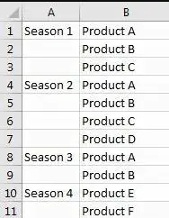
And we want to count the total product type in one year, how can we do count?

If we just use sum formula to do count, then duplicates will be included, so we need another formula to do count excludes the duplicates. See steps below.

Table of Contents

1. Count Unique Values Excluding Duplicates by Formula in Excel
2. Count Unique Values Excluding All Duplicates by Formula in Excel
3. Video: Count Only Unique Values Excluding Duplicates
4. Related Functions

Step 1: In E2 which is saved the total product type number, enter the formula:

=SUMPRODUCT(1/COUNTIF(B1:B11,B1:B11))

Where B1:B11 is the range you want to count the unique values.

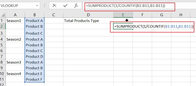
Step 2: Click Enter and get the result in E2. We can check the result is 6, and the duplicates are not included.

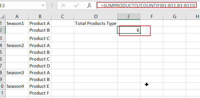
In above sample, we do count for unique values and get the result 6, because we have six products ABCDEF, and if we want to only count the unique values exclude all duplicates like product ABC (they appeared more than one season) how can we do count? See below steps.

2. Count Unique Values Excluding All Duplicates by Formula in Excel

Step 1: In E2 which is saved the total product type number, enter the formula:

=SUM(IF(FREQUENCY(MATCH(B1:B11,B1:B11,0),ROW(B1:B11)-ROW(B1)+1)=1,1))

Where B1:B11 is the range you want to count the unique values.

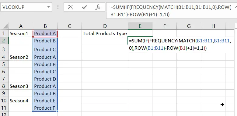
Step2: Click Enter and get the result in E2. We can check the result is 3 (Product DEF are unique values and only appeared in one season).

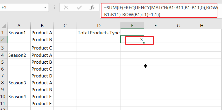
3. Video: Count Only Unique Values Excluding Duplicates

If you want to learn how to count only unique values excluding duplicates in Excel, this video will show you a simple and effective formula that you can use in any situation.

Excel SUMPRODUCT function
The Excel SUMPRODUCT function multiplies corresponding components in the given one or more arrays or ranges, and returns the sum of those products.The syntax of the SUMPRODUCT function is as below:= SUMPRODUCT (array1,[array2],…)…
Excel COUNTIF function
The Excel COUNTIF function will count the number of cells in a range that meet a given criteria. This function can be used to count the different kinds of cells with number, date, text values, blank, non-blanks, or containing specific characters.etc.= COUNTIF (range, criteria)…
Excel ROW function
The Excel ROW function returns the row number of a cell reference.The ROW function is a build-in function in Microsoft Excel and it is categorized as a Lookup and Reference Function.The syntax of the ROW function is as below:= ROW ([reference])….
Excel MATCH function
The Excel MATCH function search a value in an array and returns the position of that item.The syntax of the MATCH function is as below:= MATCH (lookup_value, lookup_array, [match_type])…
Excel IF function
The Excel IF function perform a logical test to return one value if the condition is TRUE and return another value if the condition is FALSE. The IF function is a build-in function in Microsoft Excel and it is categorized as a Logical Function.The syntax of the IF function is as below:= IF (condition, [true_value], [false_value])….
Excel SUM function
The Excel SUM function will adds all numbers in a range of cells and returns the sum of these values. You can add individual values, cell references or ranges in excel.The syntax of the SUM function is as below:= SUM(number1,[number2],…)…

Источник

Counting is an integral part of data analysis, whether you are tallying the head count of a department in your organization or the number of units that were sold quarter-by-quarter. Excel provides multiple techniques that you can use to count cells, rows, or columns of data. To help you make the best choice, this article provides a comprehensive summary of methods, a downloadable workbook with interactive examples, and links to related topics for further understanding.

Download our examples

You can download an example workbook that gives examples to supplement the information in this article. Most sections in this article will refer to the appropriate worksheet within the example workbook that provides examples and more information.

Download examples to count values in a spreadsheet

Simple counting
- Use AutoSum
- Add a Subtotal row
- Count cells in a list or Excel table column by using the SUBTOTAL function
Counting based on one or more conditions
- Video: Use the COUNT, COUNTIF, and COUNTA functions
- Count cells in a range by using the COUNT function
- Count cells in a range based on a single condition by using the COUNTIF function
- Count cells in a column based on single or multiple conditions by using the DCOUNT function
- Count cells in a range based on multiple conditions by using the COUNTIFS function
- Count based on criteria by using the COUNT and IF functions together
- Count how often multiple text or number values occur by using the SUM and IF functions together
- Count cells in a column or row in a PivotTable
Counting when your data contains blank values
- Count nonblank cells in a range by using the COUNTA function
- Count nonblank cells in a list with specific conditions by using the DCOUNTA function
- Count blank cells in a contiguous range by using the COUNTBLANK function
- Count blank cells in a non-contiguous range by using a combination of SUM and IF functions
Counting unique occurrences of values
- Count the number of unique values in a list column by using Advanced Filter
- Count the number of unique values in a range that meet one or more conditions by using IF, SUM, FREQUENCY, MATCH, and LEN functions
Special cases (count all cells, count words)
- Count the total number of cells in a range by using ROWS and COLUMNS functions
- Count words in a range by using a combination of SUM, IF, LEN, TRIM, and SUBSTITUTE functions
Displaying calculations and counts on the status bar

Simple counting

You can count the number of values in a range or table by using a simple formula, clicking a button, or by using a worksheet function.

Excel can also display the count of the number of selected cells on the Excel status bar. See the video demo that follows for a quick look at using the status bar. Also, see the section Displaying calculations and counts on the status bar for more information. You can refer to the values shown on the status bar when you want a quick glance at your data and don’t have time to enter formulas.

Video: Count cells by using the Excel status bar

Watch the following video to learn how to view count on the status bar.

Use AutoSum

Use AutoSum by selecting a range of cells that contains at least one numeric value. Then on the Formulas tab, click AutoSum > Count Numbers.

Excel returns the count of the numeric values in the range in a cell adjacent to the range you selected. Generally, this result is displayed in a cell to the right for a horizontal range or in a cell below for a vertical range.

Top of Page

Add a Subtotal row

You can add a subtotal row to your Excel data. Click anywhere inside your data, and then click Data > Subtotal.

Note: The Subtotal option will only work on normal Excel data, and not Excel tables, PivotTables, or PivotCharts.

Also, refer to the following articles:

Outline (group) data in a worksheet
Insert subtotals in a list of data in a worksheet

Top of Page

Count cells in a list or Excel table column by using the SUBTOTAL function

Use the SUBTOTAL function to count the number of values in an Excel table or range of cells. If the table or range contains hidden cells, you can use SUBTOTAL to include or exclude those hidden cells, and this is the biggest difference between SUM and SUBTOTAL functions.

The SUBTOTAL syntax goes like this:

SUBTOTAL(function_num,ref1,[ref2],…)

To include hidden values in your range, you should set the function_num argument to 2.

To exclude hidden values in your range, set the function_num argument to 102.

Top of Page

Counting based on one or more conditions

You can count the number of cells in a range that meet conditions (also known as criteria) that you specify by using a number of worksheet functions.

Video: Use the COUNT, COUNTIF, and COUNTA functions

Watch the following video to see how to use the COUNT function and how to use the COUNTIF and COUNTA functions to count only the cells that meet conditions you specify.

Top of Page

Count cells in a range by using the COUNT function

Use the COUNT function in a formula to count the number of numeric values in a range.

In the above example, A2, A3, and A6 are the only cells that contains numeric values in the range, hence the output is 3.

Note: A7 is a time value, but it contains text (a.m.), hence COUNT does not consider it a numerical value. If you were to remove a.m. from the cell, COUNT will consider A7 as a numerical value, and change the output to 4.

Top of Page

Count cells in a range based on a single condition by using the COUNTIF function

Use the COUNTIF function function to count how many times a particular value appears in a range of cells.

Top of Page

Count cells in a column based on single or multiple conditions by using the DCOUNT function

DCOUNT function counts the cells that contain numbers in a field (column) of records in a list or database that match conditions that you specify.

In the following example, you want to find the count of the months including or later than March 2016 that had more than 400 units sold. The first table in the worksheet, from A1 to B7, contains the sales data.

DCOUNT uses conditions to determine where the values should be returned from. Conditions are typically entered in cells in the worksheet itself, and you then refer to these cells in the criteria argument. In this example, cells A10 and B10 contain two conditions—one that specifies that the return value must be greater than 400, and the other that specifies that the ending month should be equal to or greater than March 31st, 2016.

You should use the following syntax:

=DCOUNT(A1:B7,»Month ending»,A9:B10)

DCOUNT checks the data in the range A1 through B7, applies the conditions specified in A10 and B10, and returns 2, the total number of rows that satisfy both conditions (rows 5 and 7).

Top of Page

Count cells in a range based on multiple conditions by using the COUNTIFS function

The COUNTIFS function is similar to the COUNTIF function with one important exception: COUNTIFS lets you apply criteria to cells across multiple ranges and counts the number of times all criteria are met. You can use up to 127 range/criteria pairs with COUNTIFS.

The syntax for COUNTIFS is:

COUNTIFS(criteria_range1, criteria1, [criteria_range2, criteria2],…)

See the following example:

Top of Page

Count based on criteria by using the COUNT and IF functions together

Let’s say you need to determine how many salespeople sold a particular item in a certain region or you want to know how many sales over a certain value were made by a particular salesperson. You can use the IF and COUNT functions together; that is, you first use the IF function to test a condition and then, only if the result of the IF function is True, you use the COUNT function to count cells.

Notes:

The formulas in this example must be entered as array formulas. If you have opened this workbook in Excel for Windows or Excel 2016 for Mac and want to change the formula or create a similar formula, press F2, and then press Ctrl+Shift+Enter to make the formula return the results you expect. In earlier versions of Excel for Mac, use +Shift+Enter.
For the example formulas to work, the second argument for the IF function must be a number.

Top of Page

Count how often multiple text or number values occur by using the SUM and IF functions together

In the examples that follow, we use the IF and SUM functions together. The IF function first tests the values in some cells and then, if the result of the test is True, SUM totals those values that pass the test.

Example 1

The above function says if C2:C7 contains the values Buchanan and Dodsworth, then the SUM function should display the sum of records where the condition is met. The formula finds three records for Buchanan and one for Dodsworth in the given range, and displays 4.

Example 2

The above function says if D2:D7 contains values lesser than $9000 or greater than $19,000, then SUM should display the sum of all those records where the condition is met. The formula finds two records D3 and D5 with values lesser than $9000, and then D4 and D6 with values greater than $19,000, and displays 4.

Example 3

The above function says if D2:D7 has invoices for Buchanan for less than $9000, then SUM should display the sum of records where the condition is met. The formula finds that C6 meets the condition, and displays 1.

Important: The formulas in this example must be entered as array formulas. That means you press F2 and then press Ctrl+Shift+Enter. In earlier versions of Excel for Mac use +Shift+Enter.

See the following Knowledge Base articles for additional tips:

XL: Using SUM(IF()) As an Array Function Instead of COUNTIF() with AND
XL: How to Count the Occurrences of a Number or Text in a Range

Top of Page

Count cells in a column or row in a PivotTable

A PivotTable summarizes your data and helps you analyze and drill down into your data by letting you choose the categories on which you want to view your data.

You can quickly create a PivotTable by selecting a cell in a range of data or Excel table and then, on the Insert tab, in the Tables group, clicking PivotTable.

Let’s look at a sample scenario of a Sales spreadsheet, where you can count how many sales values are there for Golf and Tennis for specific quarters.

Note: For an interactive experience, you can run these steps on the sample data provided in the PivotTable sheet in the downloadable workbook.

Enter the following data in an Excel spreadsheet.
Select A2:C8
Click Insert > PivotTable.
In the Create PivotTable dialog box, click Select a table or range, then click New Worksheet, and then click OK.

An empty PivotTable is created in a new sheet.
In the PivotTable Fields pane, do the following:
1. Drag Sport to the Rows area.
2. Drag Quarter to the Columns area.
3. Drag Sales to the Values area.
4. Repeat step c.
  
  The field name displays as SumofSales2 in both the PivotTable and the Values area.
  
  At this point, the PivotTable Fields pane looks like this:
5. In the Values area, click the dropdown next to SumofSales2 and select Value Field Settings.
6. In the Value Field Settings dialog box, do the following:
  1. In the Summarize value field by section, select Count.
  2. In the Custom Name field, modify the name to Count.
  3. Click OK.
The PivotTable displays the count of records for Golf and Tennis in Quarter 3 and Quarter 4, along with the sales figures.

Top of Page

Counting when your data contains blank values

You can count cells that either contain data or are blank by using worksheet functions.

Count nonblank cells in a range by using the COUNTA function

Use the COUNTA function function to count only cells in a range that contain values.

When you count cells, sometimes you want to ignore any blank cells because only cells with values are meaningful to you. For example, you want to count the total number of salespeople who made a sale (column D).

COUNTA ignores the blank values in D3, D4, D8, and D11, and counts only the cells containing values in column D. The function finds six cells in column D containing values and displays 6 as the output.

Top of Page

Count nonblank cells in a list with specific conditions by using the DCOUNTA function

Use the DCOUNTA function to count nonblank cells in a column of records in a list or database that match conditions that you specify.

The following example uses the DCOUNTA function to count the number of records in the database that is contained in the range A1:B7 that meet the conditions specified in the criteria range A9:B10. Those conditions are that the Product ID value must be greater than or equal to 2000 and the Ratings value must be greater than or equal to 50.

DCOUNTA finds two rows that meet the conditions- rows 2 and 4, and displays the value 2 as the output.

Top of Page

Count blank cells in a contiguous range by using the COUNTBLANK function

Use the COUNTBLANK function function to return the number of blank cells in a contiguous range (cells are contiguous if they are all connected in an unbroken sequence). If a cell contains a formula that returns empty text («»), that cell is counted.

When you count cells, there may be times when you want to include blank cells because they are meaningful to you. In the following example of a grocery sales spreadsheet. suppose you want to find out how many cells don’t have the sales figures mentioned.

Note: The COUNTBLANK worksheet function provides the most convenient method for determining the number of blank cells in a range, but it doesn’t work very well when the cells of interest are in a closed workbook or when they do not form a contiguous range. The Knowledge Base article XL: When to Use SUM(IF()) instead of CountBlank() shows you how to use a SUM(IF()) array formula in those cases.

Top of Page

Count blank cells in a non-contiguous range by using a combination of SUM and IF functions

Use a combination of the SUM function and the IF function. In general, you do this by using the IF function in an array formula to determine whether each referenced cell contains a value, and then summing the number of FALSE values returned by the formula.

See a few examples of SUM and IF function combinations in an earlier section Count how often multiple text or number values occur by using the SUM and IF functions together in this topic.

Top of Page

Counting unique occurrences of values

You can count unique values in a range by using a PivotTable, COUNTIF function, SUM and IF functions together, or the Advanced Filter dialog box.

Count the number of unique values in a list column by using Advanced Filter

Use the Advanced Filter dialog box to find the unique values in a column of data. You can either filter the values in place or you can extract and paste them to a new location. Then you can use the ROWS function to count the number of items in the new range.

To use Advanced Filter, click the Data tab, and in the Sort & Filter group, click Advanced.

The following figure shows how you use the Advanced Filter to copy only the unique records to a new location on the worksheet.

In the following figure, column E contains the values that were copied from the range in column D.

Notes:

If you filter your data in place, values are not deleted from your worksheet — one or more rows might be hidden. Click Clear in the Sort & Filter group on the Data tab to display those values again.
If you only want to see the number of unique values at a quick glance, select the data after you have used the Advanced Filter (either the filtered or the copied data) and then look at the status bar. The Count value on the status bar should equal the number of unique values.

For more information, see Filter by using advanced criteria

Top of Page

Count the number of unique values in a range that meet one or more conditions by using IF, SUM, FREQUENCY, MATCH, and LEN functions

Use various combinations of the IF, SUM, FREQUENCY, MATCH, and LEN functions.

For more information and examples, see the section «Count the number of unique values by using functions» in the article Count unique values among duplicates.

Top of Page

Special cases (count all cells, count words)

You can count the number of cells or the number of words in a range by using various combinations of worksheet functions.

Count the total number of cells in a range by using ROWS and COLUMNS functions

Suppose you want to determine the size of a large worksheet to decide whether to use manual or automatic calculation in your workbook. To count all the cells in a range, use a formula that multiplies the return values using the ROWS and COLUMNS functions. See the following image for an example:

Top of Page

Count words in a range by using a combination of SUM, IF, LEN, TRIM, and SUBSTITUTE functions

You can use a combination of the SUM, IF, LEN, TRIM, and SUBSTITUTE functions in an array formula. The following example shows the result of using a nested formula to find the number of words in a range of 7 cells (3 of which are empty). Some of the cells contain leading or trailing spaces — the TRIM and SUBSTITUTE functions remove these extra spaces before any counting occurs. See the following example:

Now, for the above formula to work correctly, you have to make this an array formula, otherwise the formula returns the #VALUE! error. To do that, click on the cell that has the formula, and then in the Formula bar, press Ctrl + Shift + Enter. Excel adds a curly bracket at the beginning and the end of the formula, thus making it an array formula.

For more information on array formulas, see Overview of formulas in Excel and Create an array formula.

Top of Page

Displaying calculations and counts on the status bar

When one or more cells are selected, information about the data in those cells is displayed on the Excel status bar. For example, if four cells on your worksheet are selected, and they contain the values 2, 3, a text string (such as «cloud»), and 4, all of the following values can be displayed on the status bar at the same time: Average, Count, Numerical Count, Min, Max, and Sum. Right-click the status bar to show or hide any or all of these values. These values are shown in the illustration that follows.

Top of Page

Need more help?

You can always ask an expert in the Excel Tech Community or get support in the Answers community.

Источник

View Count. 0

Hi Guys,

A lot of people has asked me this query on How to Count Text without counting duplicates in Excel, so I have decided to write an article on it, so let us discuss first what the query is, so we all know very well how to count text in Excel, for this we have COUNTA FUNCTION

Now lets assume a situation where you wants to COUNT text but with the condition that any duplicates coming in the range will be excluded, so the way to do that is discussed in this article, so lets learn

In the given situation, you can see that we have a lot of rows containing text, though duplicates are coming in these lines

Power BI – For Beginner

Product on sale

₹199.00
Basic to Advance MS Excel Course in Hindi

Product on sale

₹499.00
Microsoft Excel – VBA Projects

Product on sale

₹1,000.00
Advance Excel – Pivot Table in Depth

Product on sale

₹249.00
Advance Excel Course

Product on sale

₹2,000.00
Excel VBA Forms in Depth

Product on sale

₹500.00
Microsoft Excel – Beginner to Intermediate

Product on sale

₹2,000.00
Conditional Formatting in Depth

Product on sale

₹375.00
Login System – Excel Man

Product on sale

₹99.00

Now, If I apply COUNTA (=COUNTA(D5:D20)) in it you can see that the result is 16

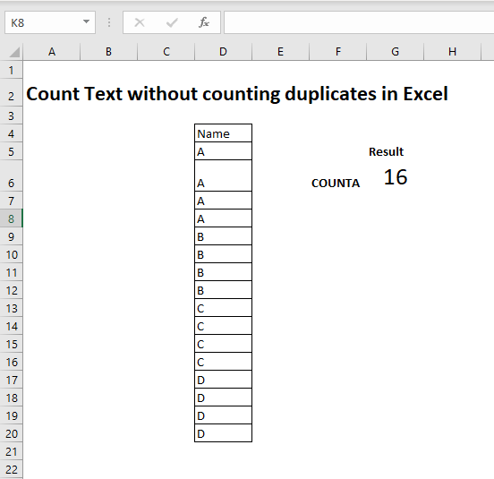
However, we want that excel should count only unique values in it, so how to do it

The answer is hidden in the question itself, as you only have to use UNIQUE Function in it & type instead of =COUNTA(D5:D20), =COUNTA(UNIQUE(D5:D20)), then we will get the result as 4, which is what we require

Источник

1. Using the array COUNTIF formula

2. Using a combination of SUM, IF, FREQUENCY, MATCH, and ROW Function

3. Using ISNUMBER Function to count numeric numbers

4. Using ISTEXT Function to count text values

5. Using Pivot Table to count text values

6. Using A Filter

6.1: Filtering for Unique Values

6.2: Removing The Duplicates

7. Using Amazing Excel Tools

8. Using A Data Model with A Pivot Table to Count Unique Values

9. Using Power Pivot

COUNTIF function in Excel — syntax and usage

Excel COUNTIF function examples

COUNTIF formula for text and numbers (exact match)

COUNTIF formulas with wildcard characters (partial match)

Count cells beginning or ending with certain characters

Excel COUNTIF for blank and non-blank cells

COUNTIF not blank

COUNTIF blank

COUNTIF greater than, less than or equal to

Using Excel COUNTIF function with dates

Excel COUNTIF with multiple criteria

COUNTIF — COUNTIF to count numbers within a range

COUNTIF + COUNTIF to count cells with multiple OR criteria

Using COUNTIF function to find duplicates and unique values

Example 1. Find and count duplicates in 1 column

Example 2. Count duplicates between two columns

Example 3. Count duplicates and unique values in a row

Excel COUNTIF — frequently asked questions and issues

1. COUNTIF on a non-contiguous range of cells

2. Ampersand and quotes in COUNTIF formulas

3. COUNTIF for formatted (color coded) cells

4. #NAME? error in the COUNTIF formula

5. Excel COUNTIF formula not working

You may also be interested in

Excel: featured articles

Table of contents

2. Count Unique Values Excluding All Duplicates by Formula in Excel

3. Video: Count Only Unique Values Excluding Duplicates

Download our examples

In this article

Simple counting

Video: Count cells by using the Excel status bar

Use AutoSum

Add a Subtotal row

Count cells in a list or Excel table column by using the SUBTOTAL function

Counting based on one or more conditions

Video: Use the COUNT, COUNTIF, and COUNTA functions

Count cells in a range by using the COUNT function

Count cells in a range based on a single condition by using the COUNTIF function

Count cells in a column based on single or multiple conditions by using the DCOUNT function

Count cells in a range based on multiple conditions by using the COUNTIFS function

Count based on criteria by using the COUNT and IF functions together

Count how often multiple text or number values occur by using the SUM and IF functions together

Count cells in a column or row in a PivotTable

Counting when your data contains blank values

Count nonblank cells in a range by using the COUNTA function

Count nonblank cells in a list with specific conditions by using the DCOUNTA function

Count blank cells in a contiguous range by using the COUNTBLANK function

Count blank cells in a non-contiguous range by using a combination of SUM and IF functions

Counting unique occurrences of values

Count the number of unique values in a list column by using Advanced Filter

Count the number of unique values in a range that meet one or more conditions by using IF, SUM, FREQUENCY, MATCH, and LEN functions

Special cases (count all cells, count words)

Count the total number of cells in a range by using ROWS and COLUMNS functions

Count words in a range by using a combination of SUM, IF, LEN, TRIM, and SUBSTITUTE functions

Displaying calculations and counts on the status bar

Need more help?