
Use the DATEDIF function when you want to calculate the difference between two dates. First put a start date in a cell, and an end date in another. Then type a formula like one of the following.
Warning: If the Start_date is greater than the End_date, the result will be #NUM!.
Difference in days
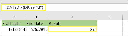
In this example, the start date is in cell D9, and the end date is in E9. The formula is in F9. The “d” returns the number of full days between the two dates.
Difference in weeks
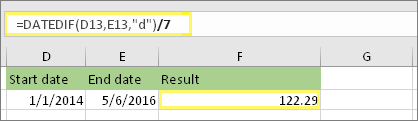
In this example, the start date is in cell D13, and the end date is in E13. The “d” returns the number of days. But notice the /7 at the end. That divides the number of days by 7, since there are 7 days in a week. Note that this result also needs to be formatted as a number. Press CTRL + 1. Then click Number > Decimal places: 2.
Difference in months

In this example, the start date is in cell D5, and the end date is in E5. In the formula, the “m” returns the number of full months between the two days.
Difference in years
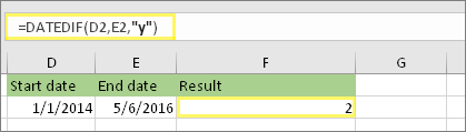
In this example, the start date is in cell D2, and the end date is in E2. The “y” returns the number of full years between the two days.
Calculate age in accumulated years, months, and days
You can also calculate age or someone’s time of service. The result can be something like “2 years, 4 months, 5 days.”
1. Use DATEDIF to find the total years.
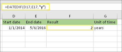
In this example, the start date is in cell D17, and the end date is in E17. In the formula, the “y” returns the number of full years between the two days.
2. Use DATEDIF again with “ym” to find months.
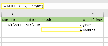
In another cell, use the DATEDIF formula with the “ym” parameter. The “ym” returns the number of remaining months past the last full year.
3. Use a different formula to find days.
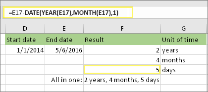
Now we need to find the number of remaining days. We’ll do this by writing a different kind of formula, shown above. This formula subtracts the first day of the ending month (5/1/2016) from the original end date in cell E17 (5/6/2016). Here’s how it does this: First the DATE function creates the date, 5/1/2016. It creates it using the year in cell E17, and the month in cell E17. Then the 1 represents the first day of that month. The result for the DATE function is 5/1/2016. Then, we subtract that from the original end date in cell E17, which is 5/6/2016. 5/6/2016 minus 5/1/2016 is 5 days.
Warning: We don’t recommend using the DATEDIF «md» argument because it may calculate inaccurate results.
4. Optional: Combine three formulas in one.
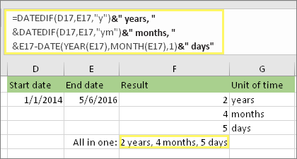
You can put all three calculations in one cell like this example. Use ampersands, quotes, and text. It’s a longer formula to type, but at least it’s all in one. Tip: Press ALT+ENTER to put line breaks in your formula. This makes it easier to read. Also, press CTRL+SHIFT+U if you can’t see the whole formula.
Download our examples
Other date and time calculations
As you saw above, the DATEDIF function calculates the difference between a start date and an end date. However, instead of typing specific dates, you can also use the TODAY() function inside the formula. When you use the TODAY() function, Excel uses your computer’s current date for the date. Keep in mind this will change when the file is opened again on a future day.
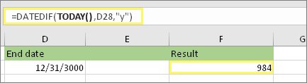
Please note that at the time of this writing, the day was October 6, 2016.
Use the NETWORKDAYS.INTL function when you want to calculate the number of workdays between two dates. You can also have it exclude weekends and holidays too.
Before you begin: Decide if you want to exclude holiday dates. If you do, type a list of holiday dates in a separate area or sheet. Put each holiday date in its own cell. Then select those cells, select Formulas > Define Name. Name the range MyHolidays, and click OK. Then create the formula using the steps below.
1. Type a start date and an end date.
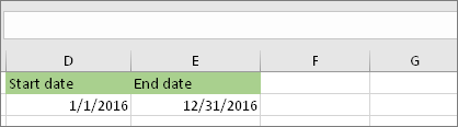
In this example, the start date is in cell D53 and the end date is in cell E53.
2. In another cell, type a formula like this:
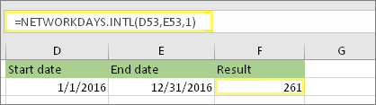
Type a formula like the above example. The 1 in the formula establishes Saturdays and Sundays as weekend days, and excludes them from the total.
Note: Excel 2007 doesn’t have the NETWORKDAYS.INTL function. However, it does have NETWORKDAYS. The above example would be like this in Excel 2007: =NETWORKDAYS(D53,E53). You don’t specify the 1 because NETWORKDAYS assumes the weekend is on Saturday and Sunday.
3. If necessary, change the 1.
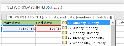
If Saturday and Sunday are not your weekend days, then change the 1 to another number from the IntelliSense list. For example, 2 establishes Sundays and Mondays as weekend days.
If you are using Excel 2007, skip this step. Excel 2007’s NETWORKDAYS function always assumes the weekend is on Saturday and Sunday.
4. Type the holiday range name.

If you created a holiday range name in the “Before you begin” section above, then type it at the end like this. If you don’t have holidays, you can leave the comma and MyHolidays out. If you are using Excel 2007, the above example would be this instead: =NETWORKDAYS(D53,E53,MyHolidays).
Tip: If you don’t want to reference a holiday range name, you can also type a range instead, like D35:E:39. Or, you could type each holiday inside the formula. For example if your holidays were on January 1 and 2 of 2016, you’d type them like this: =NETWORKDAYS.INTL(D53,E53,1,{«1/1/2016″,»1/2/2016»}). In Excel 2007, it would look like this: =NETWORKDAYS(D53,E53,{«1/1/2016″,»1/2/2016»})
You can calculate elapsed time by subtracting one time from another. First put a start time in a cell, and an end time in another. Make sure to type a full time, including the hour, minutes, and a space before the AM or PM. Here’s how:
1. Type a start time and end time.
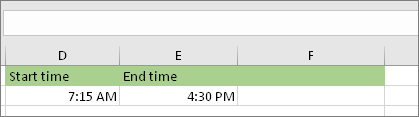
In this example, the start time is in cell D80 and the end time is in E80. Make sure to type the hour, minute, and a space before the AM or PM.
2. Set the h:mm AM/PM format.
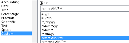
Select both dates and press CTRL + 1 (or  + 1 on the Mac). Make sure to select Custom > h:mm AM/PM, if it isn’t already set.
3. Subtract the two times.
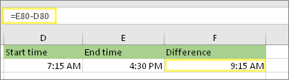
In another cell, subtract the start time cell from the end time cell.
4. Set the h:mm format.
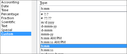
Press CTRL + 1 (or + 1 on the Mac). Choose Custom > h:mm so that the result excludes AM and PM.
To calculate the time between two dates and times, you can simply subtract one from the other. However, you must apply formatting to each cell to ensure that Excel returns the result you want.
1. Type two full dates and times.
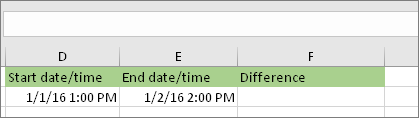
In one cell, type a full start date/time. And in another cell, type a full end date/time. Each cell should have a month, day, year, hour, minute, and a space before the AM or PM.
2. Set the 3/14/12 1:30 PM format.

Select both cells, and then press CTRL + 1 (or + 1 on the Mac). Then select Date > 3/14/12 1:30 PM. This isn’t the date you’ll set, it’s just a sample of how the format will look. Note that in versions prior to Excel 2016, this format might have a different sample date like 3/14/01 1:30 PM.
3. Subtract the two.
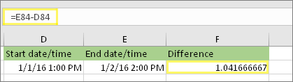
In another cell, subtract the start date/time from the end date/time. The result will probably look like a number and decimal. You’ll fix that in the next step.
4. Set the [h]:mm format.
![Format Cells dialog, Custom command, [h]:mm type](https://support.content.office.net/en-us/media/2edbd461-d4c5-49a7-a5a2-b6d9329c0411.png)
Press CTRL + 1 (or + 1 on the Mac). Select Custom. In the Type box, type [h]:mm.
Related Topics
DATEDIF function
NETWORKDAYS.INTL function
NETWORKDAYS
More date and time functions
Calculate the difference between two times
In this example, the goal is to count the number of cells in column D that contain dates that are between two variable dates in G4 and G5. This problem can be solved with the COUNTIFS function or the SUMPRODUCT function, as explained below. For convenience, the worksheet contains two named ranges: date (D5:D16) and amount (C5:C16). The named range amount is not used to count dates, but can be used to sum amounts between the same dates, as seen below.
Note: Excel dates are large serial numbers so, at the core, this problem is about counting numbers that fall into a specific range. In other words, SUMIFS and SUMPRODUCT don’t care about the dates, they only care about the numbers underneath the dates. If you like, you can see the numbers underneath by temporarily formatting the dates with the General number format.
COUNTIFS function
The COUNTIFS function is designed to count cells that meet multiple conditions. In this case, we need to provide two conditions: (1) the date is greater than or equal to G4 and (2) the date is less than or equal to G5. COUNTIFS accepts conditions as range/criteria pairs, so the conditions are entered like this:
date,">="&G4 // greater than or equal to G4
date,"<="&G5 // less than or equal to G5
The final formula looks like this:
=COUNTIFS(date,">="&G4,date,"<="&G5)
Note that the logical operators «>=» and «<=» must be entered as text and surrounded by double quotes. This means we must use concatenation with the ampersand operator (&) to join the operators to the dates in cell G4 and cell G5. This syntax is specific to a group of eight functions in Excel.
SUMPRODUCT function
This problem can also be solved with the SUMPRODUCT function which allows a cleaner syntax:
=SUMPRODUCT((date>=G4)*(date<=G5))
This is an example of using Boolean algebra in Excel. Because the named range date contains 12 dates, each expression inside SUMPRODUCT returns an array with 12 TRUE or FALSE values. When these two arrays are multiplied together, they return an array of 1s and 0s. After multiplication, we have:
=SUMPRODUCT({0;0;1;1;1;1;0;0;0;0;0;0})
SUMPRODUCT then returns the sum of the elements in the array, which is 4.
Sum amounts between dates
To sum the amounts on dates between G4 and G5 in this worksheet, you can use the SUMIFS function like this:
=SUMIFS(amount,date,">="&G4,date,"<="&G5)
The conditions in SUMIFS are the same as in COUNTIFS, but SUMIFS also accepts the range to sum as the first argument. The result is $630.
To sum the amounts for dates between G4 and G5, you can use SUMPRODUCT like this:
=SUMPRODUCT((date>=G4)*(date<=G5)*amount)
Here again, the conditions are the same as the original SUMPRODUCT formula above, but we have extended the formula to multiply by amount. This formula simplifies to:
=SUMPRODUCT({0;0;1;1;1;1;0;0;0;0;0;0}*{180;120;105;100;220;205;225;140;180;200;240;235})
The zeros in the first array effectively cancel out the amounts for dates that don’t meet criteria:
=SUMPRODUCT({0;0;105;100;220;205;0;0;0;0;0;0})
and SUMPRODUCT returns $630 as a final result.
You can use the COUNTIFS function to count the number of cells between two dates of an Excel file. In this example, the COUNTIF function isn’t suitable because you cannot use COUNTIF for multiple criteria, and we want to count the number of Excel records that fall between two dates.

Step by step COUNTIFS formula with two dates
- Type =COUNTIFS(
- Select or type the range reference for criteria_range1. In my example, I used a named range: Birthday.
- Insert criteria1. I wanted to count all birth dates after January 1st, 1985, so I inserted “>=”&DATE(E3,1,1) where cell E3 contains the year 1985.
- Select your date range again. Since we want to apply two criteria for the same data set, you will need to select the same range again.
- Insert criteria2, which is the maximum date we are interested in. In my case, I wanted to count the birth dates which occurred during 1985, which means a maximum date of December 31st, 1985, so I used
"<="&DATE(E3,12,31). - Type ) and then press Enter to complete the COUNTIFS formula.
COUNTIFS with dates – The Excel syntax
COUNTIFS(criteria_range1, criteria1, [criteria_range2, criteria2]…)
where:
criteria_range1 – the first range to compare against your criteria (Required)
criteria1 – The criteria to use on range1. It can be a number, expression, cell reference, or text that defines which cells are counted (Required)
criteria_range2 – the second range to compare against your criteria (Optional)
criteria2 – The criteria to use on range2. It can be a number, expression, cell reference, or text that defines which cells are counted (Optional)
In our example, cell F3 contains the following formula to count if the date is between two dates:=COUNTIFS(Birthday, ">="&DATE(E3,1,1), Birthday, "<="&DATE(E3,12,31))
How to use this COUNTIFS formula with multiple criteria
Since we need to check for two conditions, the COUNTIFS function is appropriate because this Excel function can easily count the number of entries between two cell values. To add the date, you can either select it from a cell or create it using the DATE function as I did below.

The first condition in cell F3 Birthday,">="&DATE(E3,1,1) checks if the birth date in the COUNTIFS date range is greater than or equal to January 1st, 1985, while the second one Birthday,"<="&DATE(E3,12,31) checks if the birth date is less than or equal to December 31st, 1985. The COUNTIFS function will return the number of cells that have dates between the two specified days if both COUNTIFS criteria are met.
When using COUNTIFS with dates, it’s important to remember to use the same COUNTIFS date range. Please note that the range “Birthday” contains cells C3:C26 from the table. This means that you need to use the same cell reference for both criteria, or else Excel will return the #VALUE! error message.
Since the logical operators ">=" and "<=" need to be entered as text between double quotes, we have to use the symbol & to concatenate the operator with each date. If you skip this step, Excel will not be able to understand your formula and will display an error message.
The following formula counts the cells between two dates by referencing the cells directly, without using the DATE function. I’ve used the same conditions: ">="&E3 and "<="&F3 and the result is the same as in the previous example.

You can also use this formula to count cells between two numbers in the same way you are using COUNTIFS with two dates.
What to do next?
In this article, I’ve shown you two examples of how to count cells between two dates using the COUNTIFS function. While this can be useful at your job, I encourage you to learn more by reading some of the following articles:
- How to count cells equal to a specific value
- How to sum sales by year
- How to separate first and last name
- How to count cells that contain odd numbers
- How to subtotal by item type
- How to use an IF function with multiple conditions
If you still struggle and have additional questions about how to use COUNTIFS with date ranges and multiple criteria, please let me know by posting a comment.
In this article, we will learn about how to Count cells between dates using COUNTIFS in Excel.
The COUNTIFS function gets the count dates that meet multiple criteria.
Syntax:
=COUNTIFS(Range ,»>=» & date1, Range, «<=» & date2)
Range : Set of values
& : operator used to concatenate other operator.
Let’s understand this function using it an example.
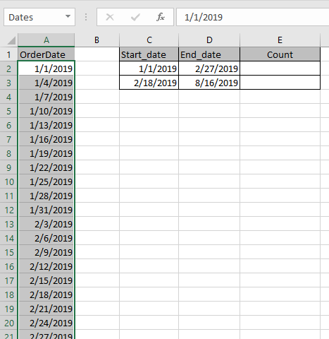
Here we have a list of dates from A2 : A245 named “Dates”.
We need to find count the fields which matches dates between the dates.
Use the Formula in E2 cell.
=COUNTIFS(Dates, «>=» & C2, Dates, «<=» & D2)
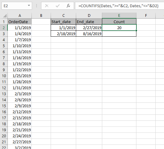
As you can see the formula to find the dates between the dates worked and it gives the output 20. That means there are 20 cells which have dates between 1/1/2019 & 2/27/2019.
Now the formula for E3 cell.
=COUNTIFS(Dates,»>=»&C3, Dates,»<=»&D3)
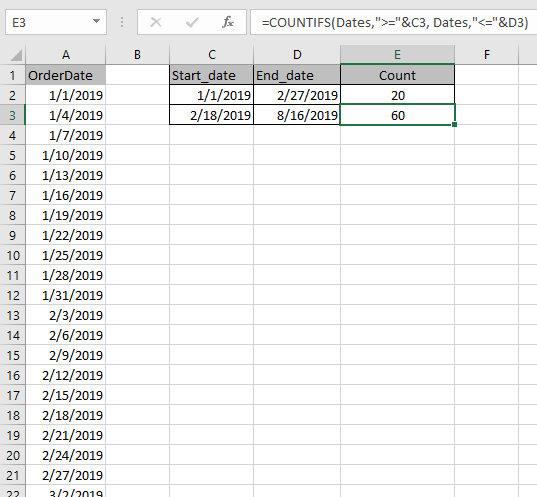
The formula returns 60. So,there are 60 dates between 2/18/2019 & 8/16/2019.
Hope you understood how to Count cells between dates in Excel. Explore more articles on Excel COUNT function here. Please feel free to state your query or feedback for the above article.
Related Articles:
How to use the DAYS function in Excel
How to Count Days in Month in Excel
Calculate days,months and years in Excel
Calculate days, years and months from certain date in Excel
Popular Articles
50 Excel Shortcut to Increase Your Productivity : Get faster at your task. These 50 shortcuts will make you work even faster on Excel.
How to use the VLOOKUP Function in Excel : This is one of the most used and popular functions of excel that is used to lookup value from different ranges and sheets.
How to use the COUNTIF function in Excel : Count values with conditions using this amazing function. You don’t need to filter your data to count specific values. Countif function is essential to prepare your dashboard.
How to use the SUMIF Function in Excel : This is another dashboard essential function. This helps you sum up values on specific conditions.
Part of Excel norms is working with numbers and dates because that is Excel’s forte. Where dates make the central part of the data, you may be working on them to add days, months, or years to them or to find the difference between them in days, months, and years.
We’ll walk you through counting the number of weeks between two dates today. By the end of this tutorial, you’ll learn counting whole weeks, nearest whole weeks, and weeks and days between dates, tied up together with a couple of Excel tricks.
Let’s get counting!
 1")
Counting Weeks Between Dates
Let’s learn first how we can calculate the number of weeks between two dates in Excel. We can then take things up a notch and calculate weeks and days between two dates.
Counting Whole Weeks
Let’s start with plain vanilla and get the add-ins to come in later. The first thing we are going to do is compute the difference in weeks between the dates with a bit of smoothing over using the INT function. The INT function rounds a number down to the nearest integer. Look at the formula below used on an example and we’ll show you why we would like to have the INT function to count weeks between dates:
=INT((D3-C3)/7)
We take the end date (in cell D3) first and subtract the start date (C3) from it. D3-C3 gives us the answer in days i.e. 14. D3-C3 is then divided by 7 so we get the answer in weeks instead and so, we arrive at 2.
This first instance was straightforward but if we look at C4 and D4, there is a difference of 20 days, and divided by 7, it gives 2.85714 and beyond. For such instances, we have the INT function ready in the formula to round the number down to the nearest whole number. Therefore, we get 2 as the result in the second instance even though it is closer to 3. This is because our objective is to count the complete weeks that have lapsed between the two dates.
 2")
The numerically logical way of calculating the difference between dates is to subtract the earlier date from the later date because the other way around would incur a minus sign. That can be tackled with the ABS function, which ignores the sign of a number. Now if you were subtracting the later date from the earlier date, this would be the formula to use:
=ABS(ROUNDDOWN((C3-D3)/7,0))
As you can see, we haven’t just added the ABS function, but we’ve also replaced the INT function with the ROUNDDOWN function. ROUNDDOWN will round the outcome of C3-D3)/7 down and also requires the number of decimal places you want. Since we want an integer, ROUNDDOWN’s second argument is 0. The end date is being subtracted. Therefore, the integer will carry a minus sign. The ABS function returns the value without its sign.
 3")
That is what is going on in the formula. Let us tell you why you can’t extend the INT formula while dealing with minus signs. INT rounds the number down to the nearest integer so if we are at -2.85, INT will round it down to -3. The ROUNDDOWN function rounds the number down toward 0. Hence, negative figures won’t be rounded down to the greater negative figure but would be rounded off close to 0 i.e. -2.
Nearest Whole Weeks
Previously we were counting the whole weeks between two dates. Now we’ll show you how to calculate the difference that is closer to the nearest whole number of weeks. Just a slight change in the formula from above should do it. Note the following formula:
=ROUND((D3-C3)/7,0)
Subtracting the dates, dividing them by 7, and maintaining that we don’t want any decimal places, the ROUND function rounds the number up or down to the closest digit and the mentioned number of digits. Looking at the results we can note in the second instance that 2.85 has been rounded up to 3 instead of 2.
 4")
Adding Text
How many times have you answered purely numerically in your math classes, to have the teacher ask you «5 what? 5 donkeys, 5 pizzas, 5 shoes?». Where the unit of measurement is embarrassingly important, here’s how to add the relevant text to the outcome. Use the following formula:
=INT((D3-C3)/7)&" weeks"
We’ve taken our first and plain vanilla formula of the day and extended it with the & operator and the text » weeks» enclosed in double quotes. Be sure to add the space before the text so you don’t get 2weeks in the result.
 5")
Happy teachers, happy days.
Note: The results of the formula have snapped from right alignment to left as they have become text values after adding text. Avoid adding text in the same cell if you want to further use the resulting value in calculations and number formulas.
Counting Weeks and Days Between Dates
Building up the formula, we’re not just going to aim to get the difference between the dates in weeks now but in weeks and days. For the «days» element, the MOD function will calculate the remaining days. The MOD function returns the remainder when two numbers are divided. This formula will return whole weeks and the remaining days:
=INT((D3-C3)/7)&" weeks "&MOD(D3-C3,7)&" days"
We’ll carry forward the last formula where we added text to the full weeks that passed between the dates in C3 and D3. Now to add the days, the & operator has concatenated the result of the MOD function. MOD subtracts C3 from D3 and the divisor is provided as 7; exactly like we have been doing with the INT formula i.e. D3-C3)/7. This expression gives us the whole weeks and the MOD function will give us the remainder of this expression, that is the remainder after the whole weeks.
C3 and D3 are exactly two weeks apart so we have 0 days in the first instance; » days» added as text after the MOD function with the & operator. Mind the right use of the space character in the text strings added in the formula. You may choose to add punctuation marks too such as the comma.
In the second instance, the gap between the dates is of 20 days the INT function returns 2 and the MOD function returns 6. That makes 2 weeks 6 days: spot on!
 6")
Adjustment for 0 Weeks
Just now you saw that C3 and D3 in our case example are giving us the difference of 2 weeks and 0 days, 0 days looking a bit odd if not a lot. Now with the plain vanilla going fully topped and loaded, we’re getting the last add-ons to the formula with the reuse of the MOD function and addition of the IF function. This formula should help you eliminate seeing 0 days in the result:
=INT((D3-C3)/7)&" weeks "&IF(MOD(D3-C3,7)=0,"",", "&MOD(D3-C3,7)&" days")
Advancing the formula from the previous section, we have added the IF function in the middle. The added bit reads that if the remainder of D3-C3 divided by 7 equals 0, then return an empty string (denoted by «»).
So the entire formula goes – number of weeks (computed by D3-C3/7), rounded down with the INT function, and suffixed with the text » weeks «. Then, if the remainder of the weeks calculation is 0, return empty text otherwise return the remainder of the weeks calculation and add » days» in text at the end.
 7")
Now you can see from the formula applied to the dataset; the number of weeks is only proceeded by the number of days if the latter doesn’t equal 0.
User Defined Function for Counting Weeks
We’re making our own formulas all the time so we’re going for the anomalous today; making our own function. Use VBA to create the function and apply it effortlessly. The function is similar to the DATEDIF function and you can find it in the steps below along with instructions to create the function:
- Go to the Developer tab > Code group > Visual Basic icon or press the Alt + F11 keys to launch the Visual Basic
 8")
- Click on the Insert tab > Module option to open a Module
 9")
- Copy the code below and paste it in the Module
'Created by ExcelTrick.com
Function WeekDiff(date1 As Date, date2 As Date) As Long
WeekDiff = DateDiff("ww", date1, date2, vbMonday)
End Function
The syntax of the function is given in the first line of the code, date1 being the earlier date and date2 being the later date. In the second line, the third argument is set by us as vbMonday which will count Monday as the first day of the week.
By leaving the third argument out, the function will consider Sunday as the first weekday by default but if you want to change that as we did, when you enter the comma after date2 in line 2, an IntelliSense list will appear with a bubble comment regarding the syntax of the DateDiff function:
 10")
- Select your favored option by double-clicking it:
 11")
- Click on the Run button in the toolbar to run the code or press the F5
You will see a Macros dialog box appear when you run the code. Enter the name of the function (Weekdiff in this case) in the given field and select the Create button.
 12")
- Close the Visual Basic editor now that the function has been created.
Back to the worksheet, it looks like nothing has changed but when you head to the target cell to enter the formula, type the name of the created function and you will see a case-sensitive entry of the function in Excel’s IntelliSense.
 13")
- Select the function and enter the formula with the earlier date and then the later date.
 14")
And you have the weeks between the dates with a created function! The number of weeks will lean towards the nearest whole figure.
Once you make good acquaintances with Excel, you’ll start finding out how little you must do on your own, which is always a good thing – especially in the Excel-verse. We hope you find the methods, tips, and tricks helpful for your task of counting weeks between dates. Keep adding to the plain vanilla as per your requirement. We’ll rope you in later with more of all that Excel jazz!