
Содержание
- Функция COUNTIF (СЧЁТЕСЛИ) в Excel. Как использовать?
- Что возвращает функция
- Синтаксис
- Аргументы функции
- Дополнительная информация
- COUNTIFS with multiple criteria and OR logic
- Related functions
- Summary
- Generic formula
- Explanation
- COUNTIFS function
- Adding another OR criteria
- Cell reference for criteria
- Wildcards and double-counting
- How to use a logical AND or OR in a SUM+IF statement in Excel
- Summary
- More Information
- Example
- References
- COUNTIF
- Numeric Criteria
- Text Tricks
- Count Booleans
- Count Errors
- And Criteria
- Or Criteria
- More about Countif
- Count Magic
Функция COUNTIF (СЧЁТЕСЛИ) в Excel. Как использовать?
Функция СЧЁТЕСЛИ (COUNTIF) в Excel используется для подсчета количества ячеек по заданному критерию.
Что возвращает функция
Функция СЧЁТЕСЛИ в Excel возвращает числовое значение обозначающее количество ячеек, отвечающих условию в заданном вами критерии.
Синтаксис
=COUNTIF(range,criteria) — английская версия
=СЧЁТЕСЛИ(где нужно искать;что нужно найти) — русская версия
Аргументы функции
- range (где нужно искать) — диапазон в рамках которого вы хотите осуществить подсчет ячеек;
- criteria (что нужно найти) — критерий, по которому все ячейки в указанном вами диапазоне будут проверены на соответствие и только после этого функция подсчитает количество ячеек.
Дополнительная информация
- Критерием может служить число, выражение, ссылка на ячейку, текст или формула;
- Критерий, указанный как текст или математический/логический символ (=,+,-,/,*) должны быть указаны в двойных кавычках.
- Подстановочные знаки могут быть использованы в качестве критерия. В Excel существует три подстановочных знака — ?, *,
.
- знак «?» — сопоставляет любой одиночный символ;
- знак «*» — сопоставляет любые дополнительные символы;
- знак «
» — используется, если нужно найти сам вопросительный знак или звездочку.
Источник
COUNTIFS with multiple criteria and OR logic

Summary
To use the COUNTIFS function with OR logic, you can use an array constant for criteria. In the example shown, the formula in H7 is:
The result is 9 since there are 6 orders that are complete and 3 orders that are pending.
Generic formula
Explanation
In this example, the goal is to use the COUNTIFS function to count data with «OR logic». The challenge is the COUNTIFS function applies AND logic by default.
COUNTIFS function
The COUNTIFS function returns the count of cells that meet one or more criteria, and supports logical operators (>, ,=) and wildcards (*,?) for partial matching. Conditions are supplied to COUNTIFS in the form of range/criteria pairs — each pair contains one range and the associated criteria for that range:
Count cells in range1 that meet criteria1.
By default, the COUNTIFS function applies AND logic. When you supply multiple conditions, ALL conditions must match in order to generate a count:
Count where range1 meets criteria1 AND range1 meets criteria2.
This means if we try to user COUNTIFS like this:
The result is zero, since the order status in column D can’t be both «complete» and «pending» at the same time. One solution is to supply multiple criteria in an array constant like this:
This will cause COUNTIFS to return two results: a count for «complete» and a count for «pending» in array like this:
In the current version of Excel, these results will spill onto the worksheet into two cells. To get a final total in one formula, we nest the COUNTIFS formula inside the SUM function like this:
COUNTIFS returns the counts directly to SUM:
And the SUM function returns the sum of the array as a final result.
Note: this is an array formula but it doesn’t require special handling in Legacy Excel when using an array constant as above. If you use a cell reference for criteria instead of an array constant, you will need to enter the formula with Control + Shift + Enter in Legacy Excel.
Adding another OR criteria
You can add one additional criteria to this formula, but you’ll need to use a single column array for criteria1 and a single row array for criteria2. So, for example, to count orders that are «Complete» or «Pending», for «Andy Garcia» or «Bob Jones», you can use:
Note we use a comma in the first array constant for a horizontal array and a semicolon for the second array constant for a vertical array. With this configuration, Excel «pairs» elements in the two array constants, and returns counts in a two dimensional array like this
| Bob Jones | Andy Garcia | |
|---|---|---|
| Complete | 1 | 1 |
| Pending | 1 | 0 |
The array result from COUNTIFS is returned directly to the SUM function:
And SUM returns the final result, which is 3 in this case.
Note: this technique will only handle two range/criteria pairs. If you have more than two criteria, consider a SUMPRODUCT formula as described here.
Cell reference for criteria
As mentioned above, you can use a cell reference for criteria in an array formula like this:
Where range is the criteria range, and B1:B2 is an example cell reference that contains criteria. This formula «just works» in the current version of Excel, which supports dynamic array formulas. However, in Legacy Excel, the formula must be entered with Control + Shift + Enter.
Wildcards and double-counting
COUNTIF and COUNTIFS support wildcards, but you need to be careful not to double-count when you have multiple «contains» conditions with OR logic. See this example for more information
Источник
How to use a logical AND or OR in a SUM+IF statement in Excel
Summary
In Microsoft Excel, when you use the logical functions AND and/or OR inside a SUM+IF statement to test a range for more than one condition, it may not work as expected. A nested IF statement provides this functionality; however, this article discusses a second, easier method that uses the following formulas.
For AND Conditions
For OR Conditions
More Information
Use a SUM+IF statement to count the number of cells in a range that pass a given test or to sum those values in a range for which corresponding values in another (or the same) range meet the specified criteria. This behaves similarly to the DSUM function in Microsoft Excel.
Example
This example counts the number of values in the range A1:A10 that fall between 1 and 10, inclusively.
To accomplish this, you can use the following nested IF statement:
The following method also works and is much easier to read if you are conducting multiple tests:
The following method counts the number of dates that fall between two given dates:
- You must enter these formulas as array formulas by pressing CTRL+SHIFT+ENTER simultaneously. On the Macintosh, press COMMAND+RETURN instead.
- Arrays cannot refer to entire columns.
With this method, you are multiplying the results of one logical test by another logical test to return TRUEs and FALSEs to the SUM function. You can equate these to:
The method shown above counts the number of cells in the range A1:A10 for which both tests evaluate to TRUE. To sum values in corresponding cells (for example, B1:B10), modify the formula as shown below:
You can implement an OR in a SUM+IF statement similarly. To do this, modify the formula shown above by replacing the multiplication sign (*) with a plus sign (+). This gives the following generic formula:
References
For more information about how to calculate a value based on a condition, click Microsoft Excel Help on the Help menu, type about calculating a value based on a condition in the Office Assistant or the Answer Wizard, and then click Search to view the topic.
Источник
COUNTIF
The powerful COUNTIF function in Excel counts cells based on one criteria. This page contains many easy to follow COUNTIF examples.
Numeric Criteria
Use the COUNTIF function in Excel to count cells that are equal to a value, count cells that are greater than or equal to a value, etc.
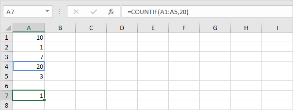
1. The COUNTIF function below counts the number of cells that are equal to 20.
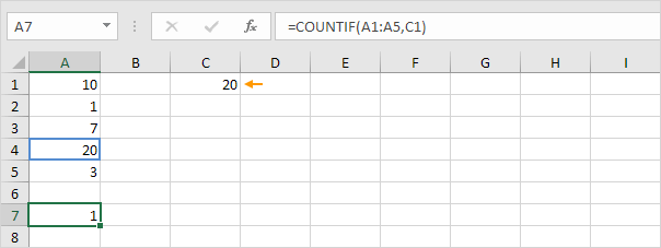
2. The following COUNTIF function gives the exact same result.
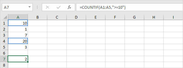
3. The COUNTIF function below counts the number of cells that are greater than or equal to 10.
4. The following COUNTIF function gives the exact same result.
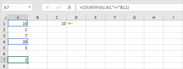
Explanation: the & operator joins the ‘greater than or equal to’ symbol and the value in cell C1.
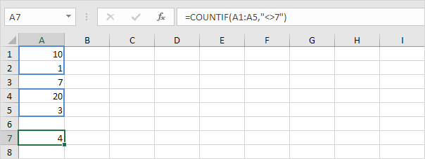
5. The COUNTIF function below counts the number of cells that are not equal to 7.
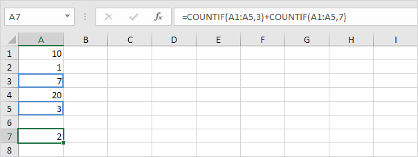
6. The COUNTIF functions below count the number of cells that are equal to 3 or 7.
Text Tricks
Use the COUNTIF function in Excel and a few tricks to count cells that contain specific text. Always enclose text in double quotation marks.
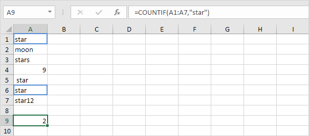
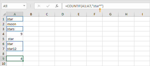
1. The COUNTIF function below counts the number of cells that contain exactly star.
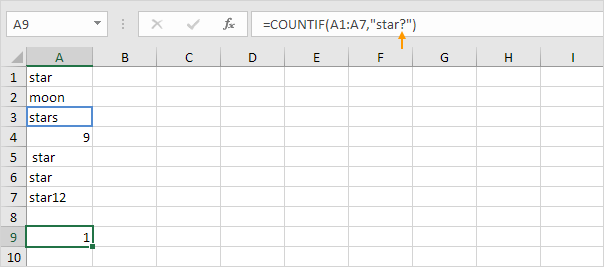
2. The COUNTIF function below counts the number of cells that contain exactly star + 1 character. A question mark (?) matches exactly one character.
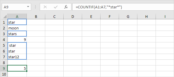
3. The COUNTIF function below counts the number of cells that contain exactly star + a series of zero or more characters. An asterisk (*) matches a series of zero or more characters.
4. The COUNTIF function below counts the number of cells that contain star in any way.
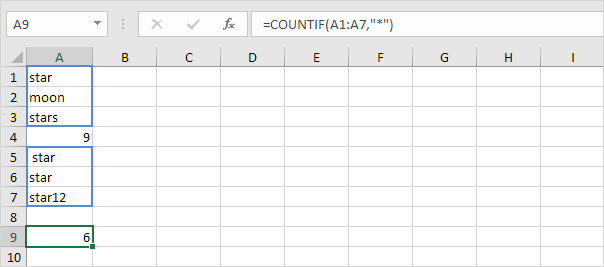
5. The COUNTIF function below counts the number of cells that contain text.
Count Booleans
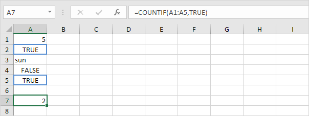
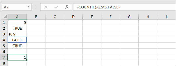
Use the COUNTIF function in Excel to count Boolean values (TRUE or FALSE).
1. The COUNTIF function below counts the number of cells that contain the Boolean TRUE.
2. The COUNTIF function below counts the number of cells that contain the Boolean FALSE.
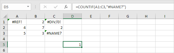
Count Errors
Use the COUNTIF function in Excel to count specific errors.
1. The COUNTIF function below counts the number of cells that contain the #NAME? error.
2. The array formula below counts the total number of errors in a range of cells.
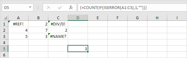
Note: finish an array formula by pressing CTRL + SHIFT + ENTER. Excel adds the curly braces <>. In Excel 365 or Excel 2021, finish by simply pressing Enter. You won’t see curly braces. Visit our page about Counting Errors for detailed instructions on how to create this array formula.
And Criteria
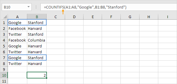
Counting with And criteria in Excel is easy. The COUNTIFS function (with the letter S at the end) in Excel counts cells based on two or more criteria.
1. For example, to count the number of rows that contain Google and Stanford, simply use the COUNTIFS function.
Or Criteria
Counting with Or criteria in Excel can be tricky.
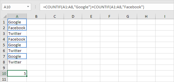
1. The COUNTIF functions below count the number of cells that contain Google or Facebook (one column). No rocket science so far.
2. However, if you want to count the number of rows that contain Google or Stanford (two columns), you cannot simply use the COUNTIF function twice (see the picture below).
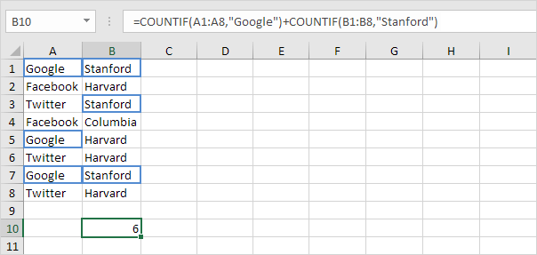
Note: rows that contain Google and Stanford are counted twice, but they should only be counted once. 4 is the answer we are looking for.
3. The array formula below does the trick.
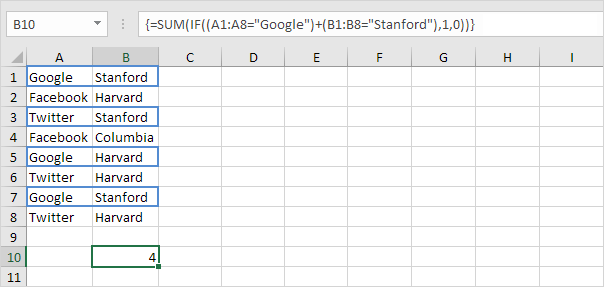
Note: finish an array formula by pressing CTRL + SHIFT + ENTER. Excel adds the curly braces <>. In Excel 365 or Excel 2021, finish by simply pressing Enter. You won’t see curly braces. Visit our page about Counting with Or Criteria for instructions on how to create this array formula.
More about Countif
The COUNTIF function is a great function. Let’s take a look at a few more cool examples.
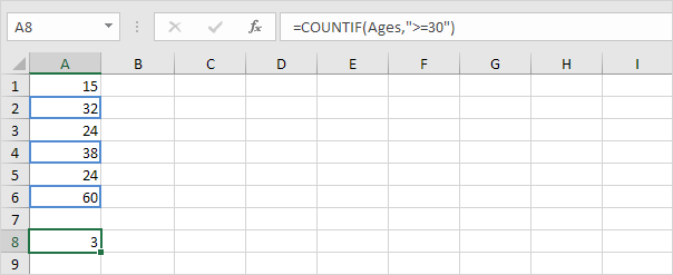
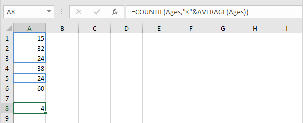
1. The COUNTIF function below uses a named range. The named range Ages refers to the range A1:A6.
2. The COUNTIF function below counts the number of cells that are less than the average of the ages (32.2).
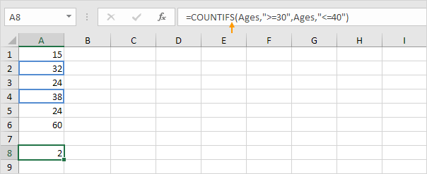
3. To count cells between two numbers, use the COUNTIFS function (with the letter S at the end).
4. Use the COUNTIF function to count how many times each value occurs in the named range Ages.
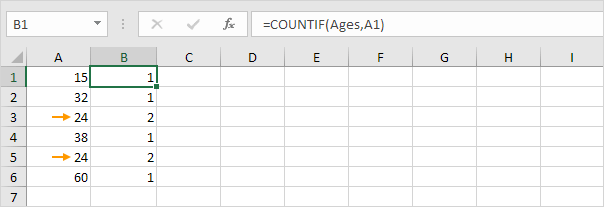
Note: cell B2 contains the formula =COUNTIF(Ages,A2), cell B3 =COUNTIF(Ages,A3), etc.
5. Add the IF function to find the duplicates.
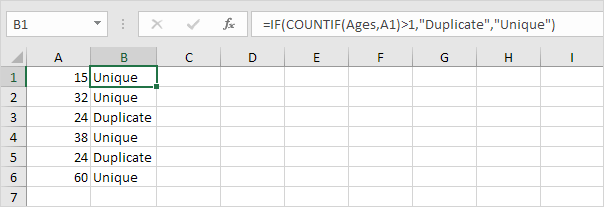
Tip: use COUNTIF and conditional formatting to find and highlight duplicates in Excel.
Count Magic
The COUNTIF function can’t count how many times a specific word occurs in a cell or range of cells. All we need is a little magic!
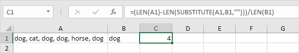
1. The formula below counts how many times the word «dog» occurs in cell A1.
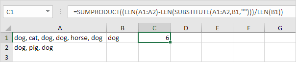
2. The formula below counts how many times the word «dog» occurs in the range A1:A2.
Note: visit our page about counting words to learn more about these formulas.
Источник
The IF function allows you to make a logical comparison between a value and what you expect by testing for a condition and returning a result if that condition is True or False.
-
=IF(Something is True, then do something, otherwise do something else)
But what if you need to test multiple conditions, where let’s say all conditions need to be True or False (AND), or only one condition needs to be True or False (OR), or if you want to check if a condition does NOT meet your criteria? All 3 functions can be used on their own, but it’s much more common to see them paired with IF functions.
Use the IF function along with AND, OR and NOT to perform multiple evaluations if conditions are True or False.
Syntax
-
IF(AND()) — IF(AND(logical1, [logical2], …), value_if_true, [value_if_false]))
-
IF(OR()) — IF(OR(logical1, [logical2], …), value_if_true, [value_if_false]))
-
IF(NOT()) — IF(NOT(logical1), value_if_true, [value_if_false]))
|
Argument name |
Description |
|
|
logical_test (required) |
The condition you want to test. |
|
|
value_if_true (required) |
The value that you want returned if the result of logical_test is TRUE. |
|
|
value_if_false (optional) |
The value that you want returned if the result of logical_test is FALSE. |
|
Here are overviews of how to structure AND, OR and NOT functions individually. When you combine each one of them with an IF statement, they read like this:
-
AND – =IF(AND(Something is True, Something else is True), Value if True, Value if False)
-
OR – =IF(OR(Something is True, Something else is True), Value if True, Value if False)
-
NOT – =IF(NOT(Something is True), Value if True, Value if False)
Examples
Following are examples of some common nested IF(AND()), IF(OR()) and IF(NOT()) statements. The AND and OR functions can support up to 255 individual conditions, but it’s not good practice to use more than a few because complex, nested formulas can get very difficult to build, test and maintain. The NOT function only takes one condition.

Here are the formulas spelled out according to their logic:
|
Formula |
Description |
|---|---|
|
=IF(AND(A2>0,B2<100),TRUE, FALSE) |
IF A2 (25) is greater than 0, AND B2 (75) is less than 100, then return TRUE, otherwise return FALSE. In this case both conditions are true, so TRUE is returned. |
|
=IF(AND(A3=»Red»,B3=»Green»),TRUE,FALSE) |
If A3 (“Blue”) = “Red”, AND B3 (“Green”) equals “Green” then return TRUE, otherwise return FALSE. In this case only the first condition is true, so FALSE is returned. |
|
=IF(OR(A4>0,B4<50),TRUE, FALSE) |
IF A4 (25) is greater than 0, OR B4 (75) is less than 50, then return TRUE, otherwise return FALSE. In this case, only the first condition is TRUE, but since OR only requires one argument to be true the formula returns TRUE. |
|
=IF(OR(A5=»Red»,B5=»Green»),TRUE,FALSE) |
IF A5 (“Blue”) equals “Red”, OR B5 (“Green”) equals “Green” then return TRUE, otherwise return FALSE. In this case, the second argument is True, so the formula returns TRUE. |
|
=IF(NOT(A6>50),TRUE,FALSE) |
IF A6 (25) is NOT greater than 50, then return TRUE, otherwise return FALSE. In this case 25 is not greater than 50, so the formula returns TRUE. |
|
=IF(NOT(A7=»Red»),TRUE,FALSE) |
IF A7 (“Blue”) is NOT equal to “Red”, then return TRUE, otherwise return FALSE. |
Note that all of the examples have a closing parenthesis after their respective conditions are entered. The remaining True/False arguments are then left as part of the outer IF statement. You can also substitute Text or Numeric values for the TRUE/FALSE values to be returned in the examples.
Here are some examples of using AND, OR and NOT to evaluate dates.

Here are the formulas spelled out according to their logic:
|
Formula |
Description |
|---|---|
|
=IF(A2>B2,TRUE,FALSE) |
IF A2 is greater than B2, return TRUE, otherwise return FALSE. 03/12/14 is greater than 01/01/14, so the formula returns TRUE. |
|
=IF(AND(A3>B2,A3<C2),TRUE,FALSE) |
IF A3 is greater than B2 AND A3 is less than C2, return TRUE, otherwise return FALSE. In this case both arguments are true, so the formula returns TRUE. |
|
=IF(OR(A4>B2,A4<B2+60),TRUE,FALSE) |
IF A4 is greater than B2 OR A4 is less than B2 + 60, return TRUE, otherwise return FALSE. In this case the first argument is true, but the second is false. Since OR only needs one of the arguments to be true, the formula returns TRUE. If you use the Evaluate Formula Wizard from the Formula tab you’ll see how Excel evaluates the formula. |
|
=IF(NOT(A5>B2),TRUE,FALSE) |
IF A5 is not greater than B2, then return TRUE, otherwise return FALSE. In this case, A5 is greater than B2, so the formula returns FALSE. |

Using AND, OR and NOT with Conditional Formatting
You can also use AND, OR and NOT to set Conditional Formatting criteria with the formula option. When you do this you can omit the IF function and use AND, OR and NOT on their own.
From the Home tab, click Conditional Formatting > New Rule. Next, select the “Use a formula to determine which cells to format” option, enter your formula and apply the format of your choice.

Using the earlier Dates example, here is what the formulas would be.

|
Formula |
Description |
|---|---|
|
=A2>B2 |
If A2 is greater than B2, format the cell, otherwise do nothing. |
|
=AND(A3>B2,A3<C2) |
If A3 is greater than B2 AND A3 is less than C2, format the cell, otherwise do nothing. |
|
=OR(A4>B2,A4<B2+60) |
If A4 is greater than B2 OR A4 is less than B2 plus 60 (days), then format the cell, otherwise do nothing. |
|
=NOT(A5>B2) |
If A5 is NOT greater than B2, format the cell, otherwise do nothing. In this case A5 is greater than B2, so the result will return FALSE. If you were to change the formula to =NOT(B2>A5) it would return TRUE and the cell would be formatted. |
Note: A common error is to enter your formula into Conditional Formatting without the equals sign (=). If you do this you’ll see that the Conditional Formatting dialog will add the equals sign and quotes to the formula — =»OR(A4>B2,A4<B2+60)», so you’ll need to remove the quotes before the formula will respond properly.
Need more help?

See also
You can always ask an expert in the Excel Tech Community or get support in the Answers community.
Learn how to use nested functions in a formula
IF function
AND function
OR function
NOT function
Overview of formulas in Excel
How to avoid broken formulas
Detect errors in formulas
Keyboard shortcuts in Excel
Logical functions (reference)
Excel functions (alphabetical)
Excel functions (by category)
I would like to include an "AND" condition for one of the conditions I have in my COUNTIFS clause.
Something like this:
=COUNTIFS(A1:A196;{"Yes"or "NO"};J1:J196;"Agree")
So, it should return the number of rows where:
(A1:A196 is either "yes" or "no") AND (J1:j196 is "agree")
![]()
apomene
14.3k9 gold badges46 silver badges71 bronze badges
asked May 14, 2014 at 13:08
![]()
You could just add a few COUNTIF statements together:
=COUNTIF(A1:A196,"yes")+COUNTIF(A1:A196,"no")+COUNTIF(J1:J196,"agree")
This will give you the result you need.
EDIT
Sorry, misread the question. Nicholas is right that the above will double count. I wasn’t thinking of the AND condition the right way. Here’s an alternative that should give you the correct results, which you were pretty close to in the first place:
=SUM(COUNTIFS(A1:A196,{"yes","no"},J1:J196,"agree"))
answered May 14, 2014 at 13:28
![]()
tmoore82tmoore82
1,8471 gold badge27 silver badges48 bronze badges
11
There is probably a more efficient solution to your question, but following formula should do the trick:
=SUM(COUNTIFS(J1:J196,"agree",A1:A196,"yes"),COUNTIFS(J1:J196,"agree",A1:A196,"no"))
answered May 14, 2014 at 13:29
![]()
Nicholas FleesNicholas Flees
1,9333 gold badges23 silver badges30 bronze badges
4
In a more general case:
N( A union B) = N(A) + N(B) - N(A intersect B)
= COUNTIFS(A1:A196,"Yes",J1:J196,"Agree")+COUNTIFS(A1:A196,"No",J1:J196,"Agree")-A1:A196,"Yes",A1:A196,"No")
![]()
answered Jun 26, 2017 at 2:12
![]()
AdelAdel
1416 bronze badges
One solution is doing the sum:
=SUM(COUNTIFS(A1:A196,{"yes","no"},B1:B196,"agree"))
or know its not the countifs but the sumproduct will do it in one line:
=SUMPRODUCT(((A1:A196={"yes","no"})*(j1:j196="agree")))
answered May 14, 2014 at 14:22
![]()
GregGreg
1415 bronze badges
Using array formula.
=SUM(COUNT(IF(D1:D5="Yes",COUNT(D1:D5),"")),COUNT(IF(D1:D5="No",COUNT(D1:D5),"")),COUNT(IF(D1:D5="Agree",COUNT(D1:D5),"")))
PRESS = CTRL + SHIFT + ENTER.
answered May 14, 2014 at 13:59
![]()
1
i found i had to do something akin to
=(countifs (A1:A196,"yes", j1:j196, "agree") + (countifs (A1:A196,"no", j1:j196, "agree"))
![]()
answered Sep 21, 2015 at 10:08
![]()
1
Author: Oscar Cronquist Article last updated on September 17, 2021
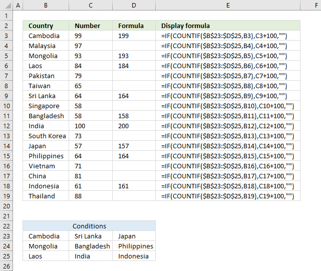
The image above demonstrates a formula that matches a value to multiple conditions, if the condition is met the formula takes the value in a corresponding cell on the same row and adds a given number.
Table of contents
- Use IF + COUNTIF to evaluate multiple conditions
- Explaining formula
- Use IF + COUNTIF to evaluate multiple conditions and different outcomes
- Explaining formula
- Get Excel file
The COUNTIF function allows you to construct a small IF formula that carries out plenty of logical expressions.
Combining the IF and COUNTIF functions also let you have more than 254 logical expressions and the effort to type the formula is minimal.
1. Use IF + COUNTIF to evaluate multiple conditions
=IF(COUNTIF($B$23:$D$25,B3),C3+100,»»)
The example shown in the above picture checks if the country in cell B3 is equal to one of the countries in cell range B23:D25.
In other words, the COUNTIF function counts how many times a specific value is found in a cell range.
If the value exists at least once in the cell range the IF function adds 100 to the value in C3. If FALSE the formula returns a blank.
Back to top
1.1 Explaining formula in cell D3
Step 1 — COUNTIF function syntax
The COUNTIF function calculates the number of cells that is equal to a condition.
COUNTIF(range, criteria)
Step 2 — Populate COUNTIF function arguments
COUNTIF(range, criteria)
becomes
COUNTIF($B$23:$D$25,B3)
range — A reference to all conditions: $B$23:$D$25
criteria — The value to match.
Step 3 — Evaluate COUNTIF function
COUNTIF($B$23:$D$25,B3)
becomes
COUNTIF({«Cambodia«, «Sri Lanka», «Japan»; «Mongolia», «Bangladesh», «Philippines»; «Laos», «India», «Indonesia»}, «Cambodia«)
and returns 1. The criteria value is found once in the array (bolded).
Step 4 — IF function syntax
The IF function returns one value if the logical test is TRUE and another value if the logical test is FALSE.
IF(logical_test, [value_if_true], [value_if_false])
Step 5 — Populate IF function arguments
IF(logical_test, [value_if_true], [value_if_false])
becomes
IF(1, C3+100, «»)
logical_test — True or False, the numerical equivalents are TRUE — 1 and False — 0 (zero). 1, in this case, is equal to TRUE.
[value_if_true] — C3+100, add 100 to value in cell C3.
[value_if_false] — «».
Step 6 — Evaluate IF function
IF(COUNTIF($B$23:$D$25, B3), C3+100, «»)
becomes
IF(1, C3+100, «»)
becomes
C3 + 100
becomes
99 + 100
and returns 199 in cell D3.
Back to top
2. Use IF + COUNTIF to evaluate multiple conditions and calculate different outcomes

The image above demonstrates a formula in cell D3 that checks if the value in cell B3 matches any of the conditions specified in cell range F4:F12. If so, add the corresponding number in cell range G4:G12 to the number in cell C3.
Formula in cell D3:
=IF(COUNTIF($F$4:$F$12, B3), C3+INDEX($G$4:$G$12, MATCH(B3, $F$4:$F$12,0)), «»)
Back to top
2.1 Explaining formula
Step 1 — Check if the value matches any of the conditions
The COUNTIF function calculates the number of cells that is equal to a condition.
COUNTIF(range, criteria)
COUNTIF($F$4:$F$12, B3)
becomes
COUNTIF({«Cambodia«; «Mongolia»; «Laos»; «Sri Lanka»; «Bangladesh»; «India»; «Japan»; «Philippines»; «Indonesia»}, «Cambodia«)
and returns 1. This means that there is one value that matches.
Step 2 — IF function
The IF function returns one value if the logical test is TRUE and another value if the logical test is FALSE.
IF(logical_test, [value_if_true], [value_if_false])
IF(COUNTIF($F$4:$F$12, B3), [value_if_true], [value_if_false])
becomes
IF(1, [value_if_true], [value_if_false])
[value_if_true] — C3+INDEX($G$4:$G$12, MATCH(B3, $F$4:$F$12,0))
[value_if_false] — «»
Step 3 — Calculate the relative position of a lookup value
The MATCH function returns the relative position of an item in an array or cell reference that matches a specified value in a specific order.
MATCH(lookup_value, lookup_array, [match_type])
MATCH(B3, $F$4:$F$12,0)
becomes
MATCH(«Cambodia», {«Cambodia»; «Mongolia»; «Laos»; «Sri Lanka»; «Bangladesh»; «India»; «Japan»; «Philippines»; «Indonesia»}, 0)
and returns 1. The lookup value is found at the first position in the array.
Step 3 — Get value
The INDEX function returns a value from a cell range, you specify which value based on a row and column number.
INDEX(array, [row_num], [column_num])
INDEX($G$4:$G$12, MATCH(B3, $F$4:$F$12,0))
becomes
INDEX($G$4:$G$12, 1)
and returns 27.
Step 4 — Add values
The plus sign lets you add numbers in an Excel formula.
C3+INDEX($G$4:$G$12, MATCH(B3, $F$4:$F$12,0))
becomes
99 + 27 equals 126.
Back to top
Get Excel *.xlsx file
Use IF + COUNTIF to perform multiple conditionsv2
Back to top
The COUNTIF function counts cells in a range that meet a given condition, referred to as criteria. COUNTIF is a common, widely used function in Excel, and can be used to count cells that contain dates, numbers, and text. Note that COUNTIF can only apply a single condition. To count cells with multiple criteria, see the COUNTIFS function.
Syntax
The generic syntax for COUNTIF looks like this:
=COUNTIF(range,criteria)The COUNTIF function takes two arguments, range and criteria. Range is the range of cells to apply a condition to. Criteria is the condition to apply, along with any logical operators that are needed.
Applying criteria
The COUNTIF function supports logical operators (>,<,<>,<=,>=) and wildcards (*,?) for partial matching. The tricky part about using the COUNTIF function is the syntax used to apply criteria. COUNTIFS is in a group of eight functions that split logical criteria into two parts, range and criteria. Because of this design, each condition requires a separate range and criteria argument, and operators in the criteria must be enclosed in double quotes («»). The table below shows examples of the syntax needed for common criteria:
| Target | Criteria |
|---|---|
| Cells greater than 75 | «>75» |
| Cells equal to 100 | 100 or «100» |
| Cells less than or equal to 100 | «<=100» |
| Cells equal to «Red» | «red» |
| Cells not equal to «Red» | «<>red» |
| Cells that are blank «» | «» |
| Cells that are not blank | «<>» |
| Cells that begin with «X» | «x*» |
| Cells less than A1 | «<«&A1 |
| Cells less than today | «<«&TODAY() |
Notice the last two examples involve concatenation with the ampersand (&) character. Any time you are using a value from another cell, or using the result of a formula in criteria with a logical operator like «<«, you will need to concatenate. This is because Excel needs to evaluate cell references and formulas first to get a value, before that value can be joined to an operator.
Basic example
In the worksheet shown above, the following formulas are used in cells G5, G6, and G7:
=COUNTIF(D5:D12,">100") // count sales over 100
=COUNTIF(B5:B12,"jim") // count name = "jim"
=COUNTIF(C5:C12,"ca") // count state = "ca"
Notice COUNTIF is not case-sensitive, «CA» and «ca» are treated the same.
Double quotes («») in criteria
In general, text values need to be enclosed in double quotes («»), and numbers do not. However, when a logical operator is included with a number, the number and operator must be enclosed in quotes, as seen in the second example below:
=COUNTIF(A1:A10,100) // count cells equal to 100
=COUNTIF(A1:A10,">32") // count cells greater than 32
=COUNTIF(A1:A10,"jim") // count cells equal to "jim"
Value from another cell
A value from another cell can be included in criteria using concatenation. In the example below, COUNTIF will return the count of values in A1:A10 that are less than the value in cell B1. Notice the less than operator (which is text) is enclosed in quotes.
=COUNTIF(A1:A10,"<"&B1) // count cells less than B1
Not equal to
To construct «not equal to» criteria, use the «<>» operator surrounded by double quotes («»). For example, the formula below will count cells not equal to «red» in the range A1:A10:
=COUNTIF(A1:A10,"<>red") // not "red"
Blank cells
COUNTIF can count cells that are blank or not blank. The formulas below count blank and not blank cells in the range A1:A10:
=COUNTIF(A1:A10,"<>") // not blank
=COUNTIF(A1:A10,"") // blank
Note: be aware that COUNTIF treats formulas that return an empty string («») as not blank. See this example for some workarounds to this problem.
Dates
The easiest way to use COUNTIF with dates is to refer to a valid date in another cell with a cell reference. For example, to count cells in A1:A10 that contain a date greater than the date in B1, you can use a formula like this:
=COUNTIF(A1:A10, ">"&B1) // count dates greater than A1
Notice we must concatenate an operator to the date in B1. To use more advanced date criteria (i.e. all dates in a given month, or all dates between two dates) you’ll want to switch to the COUNTIFS function, which can handle multiple criteria.
The safest way to hardcode a date into COUNTIF is to use the DATE function. This ensures Excel will understand the date. To count cells in A1:A10 that contain a date less than April 1, 2020, you can use a formula like this
=COUNTIF(A1:A10,"<"&DATE(2020,4,1)) // dates less than 1-Apr-2020
Wildcards
The wildcard characters question mark (?), asterisk(*), or tilde (~) can be used in criteria. A question mark (?) matches any one character and an asterisk (*) matches zero or more characters of any kind. For example, to count cells in A1:A5 that contain the text «apple» anywhere, you can use a formula like this:
=COUNTIF(A1:A5,"*apple*") // cells that contain "apple"
To count cells in A1:A5 that contain any 3 text characters, you can use:
=COUNTIF(A1:A5,"???") // cells that contain any 3 characters
The tilde (~) is an escape character to match literal wildcards. For example, to count a literal question mark (?), asterisk(*), or tilde (~), add a tilde in front of the wildcard (i.e. ~?, ~*, ~~).
OR logic
The COUNTIF function is designed to apply just one condition. However, to count cells that contain «this OR that», you can use an array constant and the SUM function like this:
=SUM(COUNTIF(range,{"red","blue"})) // red or blue
The formula above will count cells in range that contain «red» or «blue». Essentially, COUNTIF returns two counts in an array (one for «red» and one for «blue») and the SUM function returns the sum. For more information, see this example.
Limitations
The COUNTIF function has some limitations you should be aware of:
- COUNTIF only supports a single condition. If you need to count cells using multiple criteria, use the COUNTIFS function.
- COUNTIF requires an actual range for the range argument; you can’t provide an array. This means you can’t alter values in range before applying criteria.
- COUNTIF is not case-sensitive. Use the EXACT function for case-sensitive counts.
- COUNTIFS has other quirks explained in this article.
The most common way to work around the limitations above is to use the SUMPRODUCT function. In the current version of Excel, another option is to use the newer BYROW and BYCOL functions.
Notes
- Text strings in criteria must be enclosed in double quotes («»), i.e. «apple», «>32», «app*»
- Cell references in criteria are not enclosed in quotes, i.e. «<«&A1
- The wildcard characters ? and * can be used in criteria. A question mark matches any one character and an asterisk matches any sequence of characters (zero or more).
- To match a literal question mark(?) or asterisk (*), use a tilde (~) like (~?, ~*).
- COUNTIF requires a range, you can’t substitute an array.
- COUNTIF returns incorrect results when used to match strings longer than 255 characters.
- COUNTIF will return a #VALUE error when referencing another workbook that is closed.