Содержание
- COUNTIF function
- Examples
- Common Problems
- Best practices
- Need more help?
- Функция COUNTIF (СЧЁТЕСЛИ) в Excel. Как использовать?
- Что возвращает функция
- Синтаксис
- Аргументы функции
- Дополнительная информация
- COUNTIF Function
- Related functions
- Summary
- Purpose
- Return value
- Arguments
- Syntax
- Usage notes
- Syntax
- Applying criteria
- Blank cells
- Dates
- Wildcards
- OR logic
- Limitations
- Count cells equal to this or that
- Related functions
- Summary
- Generic formula
- Explanation
- COUNTIF + COUNTIF
- COUNTIF with array constant
- SUMPRODUCT function
- Double-counting risk
COUNTIF function
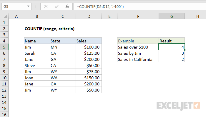
Use COUNTIF, one of the statistical functions, to count the number of cells that meet a criterion; for example, to count the number of times a particular city appears in a customer list.
In its simplest form, COUNTIF says:
=COUNTIF(Where do you want to look?, What do you want to look for?)

The group of cells you want to count. Range can contain numbers, arrays, a named range, or references that contain numbers. Blank and text values are ignored.
A number, expression, cell reference, or text string that determines which cells will be counted.
For example, you can use a number like 32, a comparison like «>32», a cell like B4, or a word like «apples».
COUNTIF uses only a single criteria. Use COUNTIFS if you want to use multiple criteria.
Examples
To use these examples in Excel, copy the data in the table below, and paste it in cell A1 of a new worksheet.
Counts the number of cells with apples in cells A2 through A5. The result is 2.
Counts the number of cells with peaches (the value in A4) in cells A2 through A5. The result is 1.
Counts the number of apples (the value in A2), and oranges (the value in A3) in cells A2 through A5. The result is 3. This formula uses COUNTIF twice to specify multiple criteria, one criteria per expression. You could also use the COUNTIFS function.
Counts the number of cells with a value greater than 55 in cells B2 through B5. The result is 2.
Counts the number of cells with a value not equal to 75 in cells B2 through B5. The ampersand (&) merges the comparison operator for not equal to (<>) and the value in B4 to read =COUNTIF(B2:B5,»<>75″). The result is 3.
=COUNTIF(B2:B5,»>=32″)-COUNTIF(B2:B5,» ) or equal to (=) 32 and less than (
Common Problems
What went wrong
Wrong value returned for long strings.
The COUNTIF function returns incorrect results when you use it to match strings longer than 255 characters.
To match strings longer than 255 characters, use the CONCATENATE function or the concatenate operator &. For example, =COUNTIF(A2:A5,»long string»&»another long string»).
No value returned when you expect a value.
Be sure to enclose the criteria argument in quotes.
A COUNTIF formula receives a #VALUE! error when referring to another worksheet.
This error occurs when the formula that contains the function refers to cells or a range in a closed workbook and the cells are calculated. For this feature to work, the other workbook must be open.
Best practices
Be aware that COUNTIF ignores upper and lower case in text strings.
Criteria aren’t case sensitive. In other words, the string «apples» and the string «APPLES» will match the same cells.
Use wildcard characters.
Wildcard characters —the question mark (?) and asterisk (*)—can be used in criteria. A question mark matches any single character. An asterisk matches any sequence of characters. If you want to find an actual question mark or asterisk, type a tilde (
) in front of the character.
For example, =COUNTIF(A2:A5,»apple?») will count all instances of «apple» with a last letter that could vary.
Make sure your data doesn’t contain erroneous characters.
When counting text values, make sure the data doesn’t contain leading spaces, trailing spaces, inconsistent use of straight and curly quotation marks, or nonprinting characters. In these cases, COUNTIF might return an unexpected value.
For convenience, use named ranges
COUNTIF supports named ranges in a formula (such as =COUNTIF( fruit,»>=32″)-COUNTIF( fruit,»>85″). The named range can be in the current worksheet, another worksheet in the same workbook, or from a different workbook. To reference from another workbook, that second workbook also must be open.
Note: The COUNTIF function will not count cells based on cell background or font color. However, Excel supports User-Defined Functions (UDFs) using the Microsoft Visual Basic for Applications (VBA) operations on cells based on background or font color. Here is an example of how you can Count the number of cells with specific cell color by using VBA.
Need more help?
You can always ask an expert in the Excel Tech Community or get support in the Answers community.
Источник
Функция COUNTIF (СЧЁТЕСЛИ) в Excel. Как использовать?
Функция СЧЁТЕСЛИ (COUNTIF) в Excel используется для подсчета количества ячеек по заданному критерию.
Что возвращает функция
Функция СЧЁТЕСЛИ в Excel возвращает числовое значение обозначающее количество ячеек, отвечающих условию в заданном вами критерии.
Синтаксис
=COUNTIF(range,criteria) — английская версия
=СЧЁТЕСЛИ(где нужно искать;что нужно найти) — русская версия
Аргументы функции
- range (где нужно искать) — диапазон в рамках которого вы хотите осуществить подсчет ячеек;
- criteria (что нужно найти) — критерий, по которому все ячейки в указанном вами диапазоне будут проверены на соответствие и только после этого функция подсчитает количество ячеек.
Дополнительная информация
- Критерием может служить число, выражение, ссылка на ячейку, текст или формула;
- Критерий, указанный как текст или математический/логический символ (=,+,-,/,*) должны быть указаны в двойных кавычках.
- Подстановочные знаки могут быть использованы в качестве критерия. В Excel существует три подстановочных знака — ?, *,
.
- знак «?» — сопоставляет любой одиночный символ;
- знак «*» — сопоставляет любые дополнительные символы;
- знак «
» — используется, если нужно найти сам вопросительный знак или звездочку.
Источник
COUNTIF Function
Summary
COUNTIF is an Excel function to count cells in a range that meet a single condition. COUNTIF can be used to count cells that contain dates, numbers, and text. The criteria used in COUNTIF supports logical operators (>, ,=) and wildcards (*,?) for partial matching.
Purpose
Return value
Arguments
- range — The range of cells to count.
- criteria — The criteria that controls which cells should be counted.
Syntax
Usage notes
The COUNTIF function counts cells in a range that meet a given condition, referred to as criteria. COUNTIF is a common, widely used function in Excel, and can be used to count cells that contain dates, numbers, and text. Note that COUNTIF can only apply a single condition. To count cells with multiple criteria, see the COUNTIFS function.
Syntax
The generic syntax for COUNTIF looks like this:
The COUNTIF function takes two arguments, range and criteria. Range is the range of cells to apply a condition to. Criteria is the condition to apply, along with any logical operators that are needed.
Applying criteria
The COUNTIF function supports logical operators (>, , =) and wildcards (*,?) for partial matching. The tricky part about using the COUNTIF function is the syntax used to apply criteria. COUNTIFS is in a group of eight functions that split logical criteria into two parts, range and criteria. Because of this design, each condition requires a separate range and criteria argument, and operators in the criteria must be enclosed in double quotes («»). The table below shows examples of the syntax needed for common criteria:
| Target | Criteria |
|---|---|
| Cells greater than 75 | «>75» |
| Cells equal to 100 | 100 or «100» |
| Cells less than or equal to 100 | » red» |
| Cells that are blank «» | «» |
| Cells that are not blank | «<>« |
| Cells that begin with «X» | «x*» |
| Cells less than A1 | » » operator surrounded by double quotes («»). For example, the formula below will count cells not equal to «red» in the range A1:A10:
Blank cellsCOUNTIF can count cells that are blank or not blank. The formulas below count blank and not blank cells in the range A1:A10: Note: be aware that COUNTIF treats formulas that return an empty string («») as not blank. See this example for some workarounds to this problem. DatesThe easiest way to use COUNTIF with dates is to refer to a valid date in another cell with a cell reference. For example, to count cells in A1:A10 that contain a date greater than the date in B1, you can use a formula like this: Notice we must concatenate an operator to the date in B1. To use more advanced date criteria (i.e. all dates in a given month, or all dates between two dates) you’ll want to switch to the COUNTIFS function, which can handle multiple criteria. The safest way to hardcode a date into COUNTIF is to use the DATE function. This ensures Excel will understand the date. To count cells in A1:A10 that contain a date less than April 1, 2020, you can use a formula like this WildcardsThe wildcard characters question mark (?), asterisk(*), or tilde ( ) can be used in criteria. A question mark (?) matches any one character and an asterisk (*) matches zero or more characters of any kind. For example, to count cells in A1:A5 that contain the text «apple» anywhere, you can use a formula like this: To count cells in A1:A5 that contain any 3 text characters, you can use: ) is an escape character to match literal wildcards. For example, to count a literal question mark (?), asterisk(*), or tilde ( ), add a tilde in front of the wildcard (i.e. OR logicThe COUNTIF function is designed to apply just one condition. However, to count cells that contain «this OR that», you can use an array constant and the SUM function like this: The formula above will count cells in range that contain «red» or «blue». Essentially, COUNTIF returns two counts in an array (one for «red» and one for «blue») and the SUM function returns the sum. For more information, see this example. LimitationsThe COUNTIF function has some limitations you should be aware of:
The most common way to work around the limitations above is to use the SUMPRODUCT function. In the current version of Excel, another option is to use the newer BYROW and BYCOL functions. Источник Count cells equal to this or that
SummaryTo count the number of cells equal to one value OR another value, you can use a formula based on the COUNTIF function. In the example shown, the formula in H6 is: where color is the named range D5:D15. The result is 7, since «red» appears 4 times and «blue» appears 3 times in the range D5:D16. See below for an explanation and for other ways to solve this problem. Note: we are using COUNTIF in this example since it does what we need, but the COUNTIFS function would work equally well. Also note that because we are counting text values «red» and «blue» are enclosed in double quotes. If we were counting numbers, the quotes would not be needed. Generic formulaExplanationIn this example, the goal is to count cells in the range D5:D15 that contain «red» or «blue». For convenience, the D5:D15 is named color. Counting cells equal to this OR that is more complicated than it first appears because there is no built-in function for counting with OR logic. The COUNTIFS function will allow multiple conditions, but all conditions are joined with AND logic. The article below explains several options. COUNTIF + COUNTIFA simple, manual way to count with OR is to use the COUNTIF function more than once: In both cases, the range argument inside COUNTIF is color (D5:D15). However, criteria is «red» in the first COUNTIF and «blue» in the second. The first COUNTIF returns 4 and the second COUNTIF returns 3, so the final result is 7. This formula works fine, but it is somewhat redundant. COUNTIF with array constantAnother way to configure COUNTIF is with an array constant that contains more than one value to use for criteria. This is the method used in the example shown above: Inside the SUM function, the COUNTIF function is given color (D5:D16) for range and <«red»,»blue»>for criteria: This causes the COUNTIF function to return two counts: one for «red» and one for «blue». These counts are returned directly to the SUM function in a single array: And SUM returns 7 as the result. In other words, COUNTIF returns multiple counts to SUM, and SUM returns a final result. This is an example of nesting one formula inside another. SUMPRODUCT functionAnother way to solve this problem is with the SUMPRODUCT function like this: This is an example of using Boolean logic. Inside SUMPRODUCT there are two expressions joined by the addition (+) operator. Because color contains 11 values, each expression creates an array with 11 TRUE and FALSE values: In the first array, the TRUE values correspond to cells that contain «red». In the second array, the TRUE values correspond to cells that contain «blue». When the two arrays are added together, the math operation converts the TRUE and FALSE values to 1s and 0s: With just one array to process SUMPRODUCT sums the items in the array and returns 7 as a result. Another way to configure SUMPRODUCT is like this: In this formula, the expression: Returns a single array with 11 rows and 2 columns. The double negative coerces the TRUE and FALSE values to 1s and 0s: And SUMPRODUCT again returns 7 as a final result. Double-counting riskWhen counting with OR logic, be aware of the risk of double-counting. In this particular example, the values «red» and «blue» are values in the same field, so there is no danger in double-counting. However, if you are counting records where one field is «red» OR another field is «blue», take care not to double-count, since both can be true at the same time in the same record. Источник Adblock |

COUNTIF function
Use COUNTIF, one of the statistical functions, to count the number of cells that meet a criterion; for example, to count the number of times a particular city appears in a customer list.
In its simplest form, COUNTIF says:
-
=COUNTIF(Where do you want to look?, What do you want to look for?)
For example:
-
=COUNTIF(A2:A5,»London»)
-
=COUNTIF(A2:A5,A4)
COUNTIF(range, criteria)
|
Argument name |
Description |
|---|---|
|
range (required) |
The group of cells you want to count. Range can contain numbers, arrays, a named range, or references that contain numbers. Blank and text values are ignored. Learn how to select ranges in a worksheet. |
|
criteria (required) |
A number, expression, cell reference, or text string that determines which cells will be counted. For example, you can use a number like 32, a comparison like «>32», a cell like B4, or a word like «apples». COUNTIF uses only a single criteria. Use COUNTIFS if you want to use multiple criteria. |
Examples
To use these examples in Excel, copy the data in the table below, and paste it in cell A1 of a new worksheet.
|
Data |
Data |
|---|---|
|
apples |
32 |
|
oranges |
54 |
|
peaches |
75 |
|
apples |
86 |
|
Formula |
Description |
|
=COUNTIF(A2:A5,»apples») |
Counts the number of cells with apples in cells A2 through A5. The result is 2. |
|
=COUNTIF(A2:A5,A4) |
Counts the number of cells with peaches (the value in A4) in cells A2 through A5. The result is 1. |
|
=COUNTIF(A2:A5,A2)+COUNTIF(A2:A5,A3) |
Counts the number of apples (the value in A2), and oranges (the value in A3) in cells A2 through A5. The result is 3. This formula uses COUNTIF twice to specify multiple criteria, one criteria per expression. You could also use the COUNTIFS function. |
|
=COUNTIF(B2:B5,»>55″) |
Counts the number of cells with a value greater than 55 in cells B2 through B5. The result is 2. |
|
=COUNTIF(B2:B5,»<>»&B4) |
Counts the number of cells with a value not equal to 75 in cells B2 through B5. The ampersand (&) merges the comparison operator for not equal to (<>) and the value in B4 to read =COUNTIF(B2:B5,»<>75″). The result is 3. |
|
=COUNTIF(B2:B5,»>=32″)-COUNTIF(B2:B5,»<=85″) |
Counts the number of cells with a value greater than (>) or equal to (=) 32 and less than (<) or equal to (=) 85 in cells B2 through B5. The result is 1. |
|
=COUNTIF(A2:A5,»*») |
Counts the number of cells containing any text in cells A2 through A5. The asterisk (*) is used as the wildcard character to match any character. The result is 4. |
|
=COUNTIF(A2:A5,»?????es») |
Counts the number of cells that have exactly 7 characters, and end with the letters «es» in cells A2 through A5. The question mark (?) is used as the wildcard character to match individual characters. The result is 2. |
Common Problems
|
Problem |
What went wrong |
|---|---|
|
Wrong value returned for long strings. |
The COUNTIF function returns incorrect results when you use it to match strings longer than 255 characters. To match strings longer than 255 characters, use the CONCATENATE function or the concatenate operator &. For example, =COUNTIF(A2:A5,»long string»&»another long string»). |
|
No value returned when you expect a value. |
Be sure to enclose the criteria argument in quotes. |
|
A COUNTIF formula receives a #VALUE! error when referring to another worksheet. |
This error occurs when the formula that contains the function refers to cells or a range in a closed workbook and the cells are calculated. For this feature to work, the other workbook must be open. |
Best practices
|
Do this |
Why |
|---|---|
|
Be aware that COUNTIF ignores upper and lower case in text strings. |
|
|
Use wildcard characters. |
Wildcard characters —the question mark (?) and asterisk (*)—can be used in criteria. A question mark matches any single character. An asterisk matches any sequence of characters. If you want to find an actual question mark or asterisk, type a tilde (~) in front of the character. For example, =COUNTIF(A2:A5,»apple?») will count all instances of «apple» with a last letter that could vary. |
|
Make sure your data doesn’t contain erroneous characters. |
When counting text values, make sure the data doesn’t contain leading spaces, trailing spaces, inconsistent use of straight and curly quotation marks, or nonprinting characters. In these cases, COUNTIF might return an unexpected value. Try using the CLEAN function or the TRIM function. |
|
For convenience, use named ranges |
COUNTIF supports named ranges in a formula (such as =COUNTIF(fruit,»>=32″)-COUNTIF(fruit,»>85″). The named range can be in the current worksheet, another worksheet in the same workbook, or from a different workbook. To reference from another workbook, that second workbook also must be open. |
Note: The COUNTIF function will not count cells based on cell background or font color. However, Excel supports User-Defined Functions (UDFs) using the Microsoft Visual Basic for Applications (VBA) operations on cells based on background or font color. Here is an example of how you can Count the number of cells with specific cell color by using VBA.
Need more help?
You can always ask an expert in the Excel Tech Community or get support in the Answers community.

See also
COUNTIFS function
IF function
COUNTA function
Overview of formulas in Excel
IFS function
SUMIF function
Need more help?
Want more options?
Explore subscription benefits, browse training courses, learn how to secure your device, and more.
Communities help you ask and answer questions, give feedback, and hear from experts with rich knowledge.
In this example, the goal is to count cells in the range D5:D15 that contain «red» or «blue». For convenience, the D5:D15 is named color. Counting cells equal to this OR that is more complicated than it first appears because there is no built-in function for counting with OR logic. The COUNTIFS function will allow multiple conditions, but all conditions are joined with AND logic. The article below explains several options.
COUNTIF + COUNTIF
A simple, manual way to count with OR is to use the COUNTIF function more than once:
=COUNTIF(color,"red") + COUNTIF(color,"blue")
In both cases, the range argument inside COUNTIF is color (D5:D15). However, criteria is «red» in the first COUNTIF and «blue» in the second. The first COUNTIF returns 4 and the second COUNTIF returns 3, so the final result is 7. This formula works fine, but it is somewhat redundant.
COUNTIF with array constant
Another way to configure COUNTIF is with an array constant that contains more than one value to use for criteria. This is the method used in the example shown above:
=SUM(COUNTIF(color,{"red","blue"}))
Inside the SUM function, the COUNTIF function is given color (D5:D16) for range and {«red»,»blue»} for criteria:
COUNTIF(color,{"red","blue"}) // returns {4,3}
This causes the COUNTIF function to return two counts: one for «red» and one for «blue». These counts are returned directly to the SUM function in a single array:
=SUM({4,3}) // returns 7
And SUM returns 7 as the result. In other words, COUNTIF returns multiple counts to SUM, and SUM returns a final result. This is an example of nesting one formula inside another.
For more complicated scenarios, see: COUNTIFS with multiple criteria and or logic
SUMPRODUCT function
Another way to solve this problem is with the SUMPRODUCT function like this:
=SUMPRODUCT((D5:D15="red")+(D5:D15="blue"))
This is an example of using Boolean logic. Inside SUMPRODUCT there are two expressions joined by the addition (+) operator. Because color contains 11 values, each expression creates an array with 11 TRUE and FALSE values:
=SUMPRODUCT({TRUE;TRUE;FALSE;FALSE;FALSE;FALSE;TRUE;FALSE;FALSE;TRUE;FALSE}+{FALSE;FALSE;TRUE;FALSE;TRUE;FALSE;FALSE;FALSE;TRUE;FALSE;FALSE})
In the first array, the TRUE values correspond to cells that contain «red». In the second array, the TRUE values correspond to cells that contain «blue». When the two arrays are added together, the math operation converts the TRUE and FALSE values to 1s and 0s:
=SUMPRODUCT({1;1;1;0;1;0;1;0;1;1;0})
With just one array to process SUMPRODUCT sums the items in the array and returns 7 as a result. Another way to configure SUMPRODUCT is like this:
=SUMPRODUCT(--(D5:D15={"red","blue"}))
In this formula, the expression:
D5:D15={"red","blue"})
Returns a single array with 11 rows and 2 columns. The double negative coerces the TRUE and FALSE values to 1s and 0s:
=SUMPRODUCT({1,0;1,0;0,1;0,0;0,1;0,0;1,0;0,0;0,1;1,0;0,0})
And SUMPRODUCT again returns 7 as a final result.
For more complex scenarios see: SUMPRODUCT with multiple criteria and OR logic and Count cells equal to one of many things.
Double-counting risk
When counting with OR logic, be aware of the risk of double-counting. In this particular example, the values «red» and «blue» are values in the same field, so there is no danger in double-counting. However, if you are counting records where one field is «red» OR another field is «blue», take care not to double-count, since both can be true at the same time in the same record.
In our article, Count Cells That Contain Specific Text, we counted each cell that contains a specific text. In this article we will learn how to count cells that contains either this or that value. In other words, counting with OR logic.
You may think that you can use COUNTIF function two times and then add them up. But that is a wrong turn. You’ll know why.
Generic Formula
“This”: it is the first text you want count in the range. It can be any text.
“That”: it is the second text that you want to count in range. It can be any text.
Range: This is the range or array containing text in which you will count for your specific texts.
Let’s see an example:
Example:
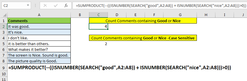
Here I have feedback comments in range A2 to A8. I want to count the number of comments containing “good” or “nice” words.
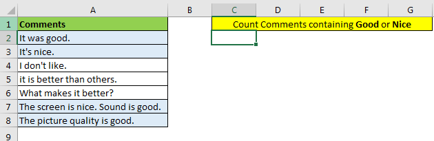
To count cells containing specific texts “good” or “nice” write this formula:
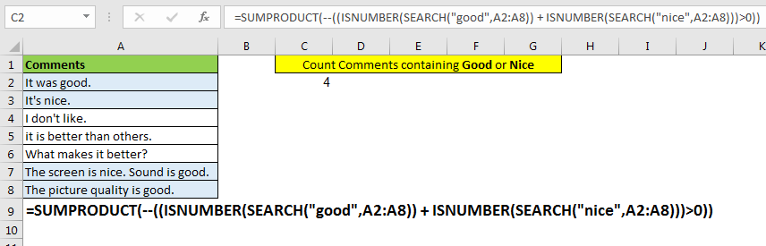
You can see that there are four comments that contain either “good” or “nice.”
How it works?
Let’s start from inside.
SEARCH(«good»,A2:A8): this part returns an array of #VALUE error and numbers, representing the position of found text. {8;#VALUE!;#VALUE!;#VALUE!;#VALUE!;30;24}
ISNUMBER(SEARCH(«good»,A2:A8)): this part of the formula checks each value in array return by SEARCH function, if it is a number or not, and returns an array of TRUE and FALSE. For this example, it returns {TRUE;FALSE;FALSE;FALSE;FALSE;TRUE;TRUE}.
ISNUMBER(SEARCH(«nice»,A2:A8)): this part of formula does the same, but this time it looks for “nice” word in cell and returns an array of the TRUE and FALSE base on cell contains the “nice.”
Next, we have added these arrays using + sign. It boolean values into 1 and 0 and adds them up. Internally it will look like this, {1;0;0;0;0;1;1}+{0;1;0;0;0;1;0}={1;1;0;0;0;2;1}.
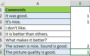
You can see that comment in A7 has both texts “nice” and “good.” And it is double-counted here. We don’t want it. So we make another comparison for converting every number into True and False.
((ISNUMBER(SEARCH(«good»,A2:A8)) + ISNUMBER(SEARCH(«nice»,A2:A8)))>0): This part of formula converts the resultant array into TRUE and FALSE. If the value is greater than 0, it is TRUE else FALSE. Here it will be {TRUE;TRUE;FALSE;FALSE;FALSE;TRUE;TRUE}.
The number of TRUE in the array is the name of the string contain “good” or “nice” words.
SUMPRODUCT(—((ISNUMBER(SEARCH(«good»,A2:A8)) + ISNUMBER(SEARCH(«nice»,A2:A8)))>0))
Next we use — negative symbols to convert them into numbers. And finally SUMPRODUCT sums up the array to return number of cells containing “good” or “nice”.
You can also use the SUM function, but then you’ll have to enter this formula as an array formula.
Why not use COUNTIFS?

Because of double counts.
If a cell contains both of the texts, then it will be counted twice, which is not correct in this scenario.
But if you want it to happen then use this formula,
=SUM(COUNTIFS(A2:A8,{«*nice*»,»*good*»}))
It will return 5 in our example. I have explained it here.
Making Case Sensitive Count
The proposed solution counts the given text irrespective of the case of letters. If you want to count case sensitive matches, then replace SEARCH function with FIND function.
The FIND function is case sensitive function. It returns the position of found text.
So yeah guys, this how you can count the number of cells that contain either this text or that. You can also click on the function names in the formula to read about that function. I have understandably elaborated them.
Related Articles:
How to Check If Cell Contains Specific Text in Excel
How to Check a list of Texts In String in Excel
Get COUNTIFS Two Criteria Match in Excel
Get COUNTIFS With OR For Multiple Criteria in Excel
Popular Articles :
50 Excel Shortcut to Increase Your Productivity : Get faster at your task. These 50 shortcuts will make you work even faster on Excel.
How to use the VLOOKUP Function in Excel : This is one of the most used and popular functions of excel that is used to lookup value from different ranges and sheets.
How to use the COUNTIF function in Excel : Count values with conditions using this amazing function. You don’t need to filter your data to count specific values. Countif function is essential to prepare your dashboard.
How to use the SUMIF Function in Excel : This is another dashboard essential function. This helps you sum up values on specific conditions.
Return to Excel Formulas List
Download Example Workbook
Download the example workbook
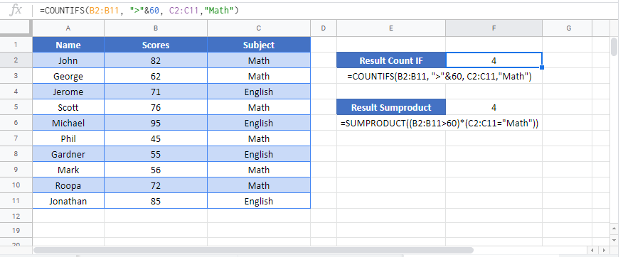
This tutorial demonstrates how to “count if” with multiple criteria using the COUNTIFS Function in Excel and Google Sheets. If your version of Excel does not support COUNTIFS, we also demonstrate how to use the SUMPRODUCT function instead.
COUNTIFS Function
The COUNTIFS Function allows you to count values that meet multiple criteria. The basic formula structure is:
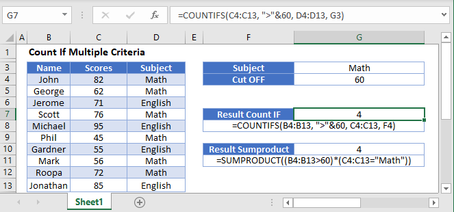
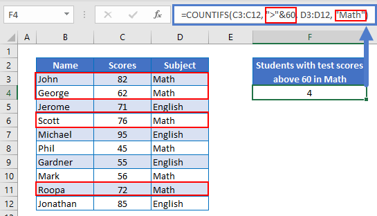
=COUNTIFS(Range 1, Condition 1, Range 2, Condition 2)Let’s look at an example. Below you will see a list containing grades for students in English and Math. Let’s count all students with test scores above 60 in Math.
=COUNTIFS(C3:C12, ">"&60, D3:D12, "Math")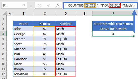
In this case, we are testing two criteria:
- If the Test Scores are greater than 60 (Range B2:B11)
- If the Subject is “Math” (Range is C2:C11)
Below, you can see that there are 4 students who scored above 60 in Math:
You can test additional conditions by adding another range and criteria. For example, if you wanted to count the number of students who scored between 60 and 80 in Math you would use this criteria:
- If the Test Scores are greater than 60
- If the Test Scores are below 80
- If the Subject is “Math”
Here are the highlighted sections where these examples are being tested.
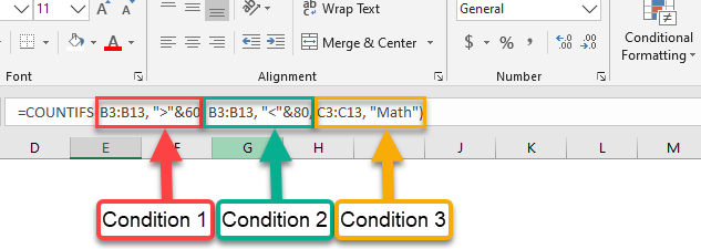
The result, in this case, is 3.
=COUNTIFS(B3:B13,">" & 60,B3:B13,"<"&80,C3:C13,"Math")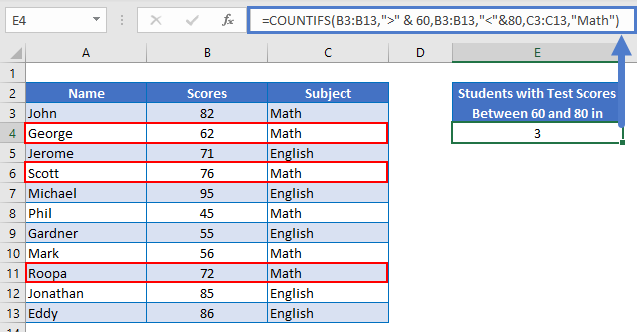
SUMPRODUCT Function
If you don’t have access to COUNTIFS, you can accomplish the same task with the SUMPRODUCT Function. The SUMPRODUCT Function opens up a world of possibilities with complex formulas (see SUMPRODUCT Tutorial). So, even if you have access to the COUNTIFS Function, you may want to start familiarizing yourself with this powerful function. It’s syntax is:
=SUMPRODUCT(Range 1=Condition 1*Range 2=Condition 2)Using the same example above, to count all students with test scores above 60 in subject “Math”, you can use this formula:
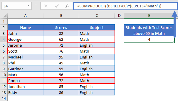
=SUMPRODUCT((B3:B13>60)*(C3:C13="Math"))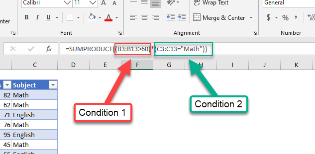
The first condition tests which values in that range are greater than 60, and the second condition tests which values in that range equal to “Math”. This gives us an array of Boolean values of 1 (TRUE) or 0 (FALSE):
=SUMPRODUCT(({82;62;71;76;95;45;55;56;72;85;86}>60)*({"Math";"Math";"English";"Math";"English";"Math";"English";"Math";"Math";"English";"English"}="Math"))=SUMPRODUCT(({TRUE;TRUE;TRUE;TRUE;TRUE;FALSE;FALSE;FALSE;TRUE;TRUE;TRUE})*({TRUE;TRUE;FALSE;TRUE;FALSE;TRUE;FALSE;TRUE;TRUE;FALSE;FALSE}))=SUMPRODUCT({1;1;0;1;0;0;0;0;1;0;0})=4The SUMPRODUCT Function then totals all items in the array, giving us the count of students who scored about 60 in math.
COUNTIFS and SUMPRODUCT for Multiple Criteria in Google Sheets
You can use the same formula structures as above in Google Sheets to count with multiple criteria.