Count if there is a value excel

COUNTIF function

Use COUNTIF, one of the statistical functions, to count the number of cells that meet a criterion; for example, to count the number of times a particular city appears in a customer list.

In its simplest form, COUNTIF says:

• =COUNTIF(Where do you want to look?, What do you want to look for?)

For example:

• =COUNTIF(A2:A5,»London»)

• =COUNTIF(A2:A5,A4)

COUNTIF(range, criteria)

Argument name	Description
range    (required)	The group of cells you want to count. Range can contain numbers, arrays, a named range, or references that contain numbers. Blank and text values are ignored. Learn how to select ranges in a worksheet.
criteria    (required)	A number, expression, cell reference, or text string that determines which cells will be counted. For example, you can use a number like 32, a comparison like «>32», a cell like B4, or a word like «apples». COUNTIF uses only a single criteria. Use COUNTIFS if you want to use multiple criteria.

Examples

To use these examples in Excel, copy the data in the table below, and paste it in cell A1 of a new worksheet.

Data	Data
apples	32
oranges	54
peaches	75
apples	86
Formula	Description
=COUNTIF(A2:A5,»apples»)	Counts the number of cells with apples in cells A2 through A5. The result is 2.
=COUNTIF(A2:A5,A4)	Counts the number of cells with peaches (the value in A4) in cells A2 through A5. The result is 1.
=COUNTIF(A2:A5,A2)+COUNTIF(A2:A5,A3)	Counts the number of apples (the value in A2), and oranges (the value in A3) in cells A2 through A5. The result is 3. This formula uses COUNTIF twice to specify multiple criteria, one criteria per expression. You could also use the COUNTIFS function.
=COUNTIF(B2:B5,»>55″)	Counts the number of cells with a value greater than 55 in cells B2 through B5. The result is 2.
=COUNTIF(B2:B5,»<>»&B4)	Counts the number of cells with a value not equal to 75 in cells B2 through B5. The ampersand (&) merges the comparison operator for not equal to (<>) and the value in B4 to read =COUNTIF(B2:B5,»<>75″). The result is 3.
=COUNTIF(B2:B5,»>=32″)-COUNTIF(B2:B5,»<=85″)	Counts the number of cells with a value greater than (>) or equal to (=) 32 and less than (<) or equal to (=) 85 in cells B2 through B5. The result is 1.
=COUNTIF(A2:A5,»*»)	Counts the number of cells containing any text in cells A2 through A5. The asterisk (*) is used as the wildcard character to match any character. The result is 4.
=COUNTIF(A2:A5,»?????es»)	Counts the number of cells that have exactly 7 characters, and end with the letters «es» in cells A2 through A5. The question mark (?) is used as the wildcard character to match individual characters. The result is 2.

Common Problems

Problem	What went wrong
Wrong value returned for long strings.	The COUNTIF function returns incorrect results when you use it to match strings longer than 255 characters. To match strings longer than 255 characters, use the CONCATENATE function or the concatenate operator &. For example, =COUNTIF(A2:A5,»long string»&»another long string»).
No value returned when you expect a value.	Be sure to enclose the criteria argument in quotes.
A COUNTIF formula receives a #VALUE! error when referring to another worksheet.	This error occurs when the formula that contains the function refers to cells or a range in a closed workbook and the cells are calculated. For this feature to work, the other workbook must be open.

Best practices

Do this	Why
Be aware that COUNTIF ignores upper and lower case in text strings.	Criteria aren’t case sensitive. In other words, the string «apples» and the string «APPLES» will match the same cells.
Use wildcard characters.	Wildcard characters —the question mark (?) and asterisk (*)—can be used in criteria. A question mark matches any single character. An asterisk matches any sequence of characters. If you want to find an actual question mark or asterisk, type a tilde (~) in front of the character. For example, =COUNTIF(A2:A5,»apple?») will count all instances of «apple» with a last letter that could vary.
Make sure your data doesn’t contain erroneous characters.	When counting text values, make sure the data doesn’t contain leading spaces, trailing spaces, inconsistent use of straight and curly quotation marks, or nonprinting characters. In these cases, COUNTIF might return an unexpected value. Try using the CLEAN function or the TRIM function.
For convenience, use named ranges	COUNTIF supports named ranges in a formula (such as =COUNTIF(fruit,»>=32″)-COUNTIF(fruit,»>85″). The named range can be in the current worksheet, another worksheet in the same workbook, or from a different workbook. To reference from another workbook, that second workbook also must be open.

Note: The COUNTIF function will not count cells based on cell background or font color. However, Excel supports User-Defined Functions (UDFs) using the Microsoft Visual Basic for Applications (VBA) operations on cells based on background or font color. Here is an example of how you can Count the number of cells with specific cell color by using VBA.

Need more help?

You can always ask an expert in the Excel Tech Community or get support in the Answers community.

See also

COUNTIFS function

IF function

COUNTA function

Overview of formulas in Excel

IFS function

SUMIF function

In this example, the goal is to use a formula to check if a specific value exists in a range. The easiest way to do this is to use the COUNTIF function to count occurences of a value in a range, then use the count to create a final result.

COUNTIF function

The COUNTIF function counts cells that meet supplied criteria. The generic syntax looks like this:

=COUNTIF(range,criteria)

Range is the range of cells to test, and criteria is a condition that should be tested. COUNTIF returns the number of cells in range that meet the condition defined by criteria. If no cells meet criteria, COUNTIF returns zero. In the example shown, we can use COUNTIF to count the values we are looking for like this

COUNTIF(data,E5)

Once the named range data (B5:B16) and cell E5 have been evaluated, we have:

=COUNTIF(data,E5)
=COUNTIF(B5:B16,"Blue")
=1

COUNTIF returns 1 because «Blue» occurs in the range B5:B16 once. Next, we use the greater than operator (>) to run a simple test to force a TRUE or FALSE result:

=COUNTIF(data,B5)>0 // returns TRUE or FALSE

By itself, the formula above will return TRUE or FALSE. The last part of the problem is to return a «Yes» or «No» result. To handle this, we nest the formula above into the IF function like this:

=IF(COUNTIF(data,E5)>0,"Yes","No")

This is the formula shown in the worksheet above. As the formula is copied down, COUNTIF returns a count of the value in column E. If the count is greater than zero, the IF function returns «Yes». If the count is zero, IF returns «No».

Slightly abbreviated

It is possible to shorten this formula slightly and get the same result like this:

=IF(COUNTIF(data,E5),"Yes","No")

Here, we have remove the «>0» test. Instead, we simply return the count to IF as the logical_test. This works because Excel will treat any non-zero number as TRUE when the number is evaluated as a Boolean.

Testing for a partial match

To test a range to see if it contains a substring (a partial match), you can add a wildcard to the formula. For example, if you have a value to look for in cell C1, and you want to check the range A1:A100 for partial matches, you can configure COUNTIF to look for the value in C1 anywhere in a cell by concatenating asterisks on both sides:

=COUNTIF(A1:A100,"*"&C1&"*")>0

The asterisk (*) is a wildcard for one or more characters. By concatenating asterisks before and after the value in C1, the formula will count the text in C1 anywhere it appears in each cell of the range. To return «Yes» or «No», nest the formula inside the IF function as above.

An alternative formula using MATCH

As an alternative, you can use a formula that uses the MATCH function with the ISNUMBER function instead of COUNTIF:

=ISNUMBER(MATCH(value,range,0))

The MATCH function returns the position of a match (as a number) if found, and #N/A if not found. By wrapping MATCH inside ISNUMBER, the final result will be TRUE when MATCH finds a match and FALSE when MATCH returns #N/A.

EXPLANATION

This tutorial shows and explains how to count cells that contain a specific value by using Excel formulas or VBA.

This tutorial provides two Excel methods that can be applied to count cells that contain a specific value in a selected range by using an Excel COUNTIF function. The first method reference to a cell that capture the value that we want to count for, whilst the second method has the value (Exceldome) directly entered into the formula.

This tutorial provides two VBA methods that can be applied to count cells that contain a specific value in a selected range. The first method reference to a cell that capture the value that we want to count for, whilst the second method has the value (Exceldome) directly entered into the VBA code.

By including asterisk (*) in front and behind the value that we are searching for it will ensure that the formula will still count a cell if there is other content, in addition to the specified value, in the cell.

FORMULA (value manually entered)
=COUNTIF(range, «*value*»)

FORMULA (value sourced from cell reference)
=COUNTIF(range, «*»&value&»*»)

ARGUMENTS
range: The range of cells you want to count from.
value: The value that is used to determine which of the cells should be counted, from a specified range, if the cells contain this value.

I have an Excel sheet like this:

ID  | Relations
----+----------------
1   | ,
2   | ,
3   | ,1,
4   | ,1,2,
5   | ,2,
6   | ,3,
7   | ,1,2,4,
8   | ,1,2,4,5,6,
9   | ,2,4,5,1,

I want to count Relations as Related Count column — that checks if finding ,ID, in Relations is true — with a formula to achieve a result like this:

ID  | Relations     | Related Count
----+---------------+----------------
1   | ,             | 5               '>> related in: 3,4,7,8,9
2   | ,             | 5               '>> related in: 4,5,7,8,9
3   | ,1,           | 1               '>> related in: 6
4   | ,1,2,         | 3               '>> related in: 7,8,9
5   | ,2,           | 2               '>> related in: 8,9
6   | ,3,           | 1               '>> related in: 8
7   | ,1,2,4,       | 0
8   | ,1,2,4,5,6,   | 0
9   | ,2,4,5,1,     | 0

Edit:
I know how to use countif() function, Please help me in finding a formula for Related Count column.
Thanks in advance.

This Tutorial demonstrates how to use the ExcelCOUNTIF  and COUNTIFS Functions in Excel to count data that meet certain criteria.

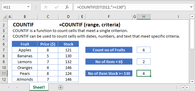
COUNTIF Function Overview

You can use the COUNTIF function in Excel to count cells that contain a specific value, count cells that are greater than or equal to a value, etc.

(Notice how the formula inputs appear)

COUNTIF Function Syntax and Arguments:

=COUNTIF(range, criteria)

range – The range of cells to count.

criteria – The criteria that controls which cells should be counted.

What is the COUNTIF function?

The COUNTIF function is one of the older functions used in spreadsheets. In simple terms, it’s great at scanning a range and telling you how many of the cells meet that condition. We’ll look at how the function works with text, numbers, and dates; as well as some of the other situations that might arise.

Basic example

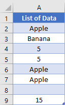
Let’s start by looking at this list of random items. We’ve got some numbers, blank cells, and some text strings.

If you wanted to know how many items an exact match to the criteria are, you can specify what you want to look for as the second argument. An example of this formula might look like

=COUNTIF(A2:A9, "Apple")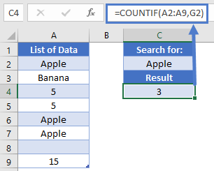

This formula would return the number 3, as there are 3 cells in our range that meet that criteria. Alternatively, we can use a cell reference instead of hardcoding a value. If we wrote “Apple” in cell G2, we could change the formula to

=COUNTIF(A2:A9, G2)

When dealing with number, it’s important to distinguish between numbers and numbers that are been stored as text. Generally, you don’t put quotation marks around numbers when writing formulas. So, to write a formula that checks for the number 5, you would write

=COUNTIF(A2:A9, 5)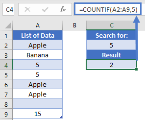

Finally, we could also check for blank cells by using a zero-length string. We would write that formula as

=COUNTIF(A2:A9, "")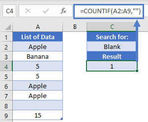

Note: This formula will count both cells that are truly empty, as well as those that are blank as the result of a formula, like an IF function.

Partial matches

The COUNTIF function supports the use of wildcards, “*” or “?”, in the criteria. Let’s look at this list of tasty bakery goods:

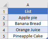
To find all the items that start with Apple, we could write “Apple*”. So, to get an answer of 3, our formula in D2 is

=COUNTIF(A2:A5, "Apple*")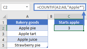

Note: The COUNTIF function is not case-sensitive, so you could also write “apple*” if you want.

Back to our baked goods, we might also want to find out how many pies we have in our list. We can find that by placing the wildcard at the beginning of our search term, and write

=COUNTIF(A2:A5, "*pie")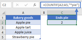

This formula gives the result of 2.

We can also use wildcards to check for any cells with text. Let’s go back to our original list of data.

To count the number of cells that have at least some text, thus not counting numbers or blank cell, we can write

=COUNTIF(A2:A9, "*")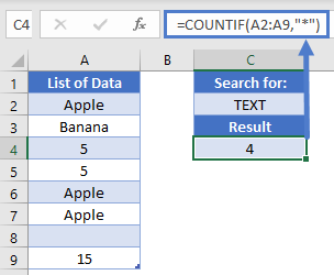

You can see that our formula correctly returns a result of 4.

Comparison operators in COUNTIF

When writing the criteria so far, we’ve been implying that our comparison operator is “=”. In fact, we could have written this:

=COUNTIF(A2:A9, "=Apple")

It’s an extra character to write out though, so it’s usually omitted. However, this means that you can use the other operators such as greater than, less than, or not equal to. Let’s look at this list of recorded ages:

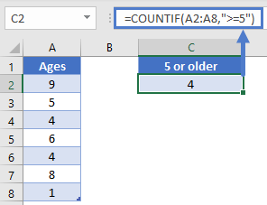
If we wanted to know how many kids are at least 5 years old, we can write out a “greater than or equal to” comparison like so:

=COUNTIF(A2:A8, ">=5")

Note: The comparison operator is always given as a text string, and thus must be inside quotation marks.

Similarly, you can also check for items that are less than a given value. If we need to find out how many are less than 8, we can write out

=COUNTIF(A2:A8, "<8")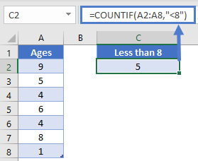

This gives us the desired result of 5. Now let’s imagine that all the 6-year old kids are going on an outing. How many kids will remain? We can figure this out by using a “not equal to” comparison like this:

=COUNTIF(A2:A8, "<>6")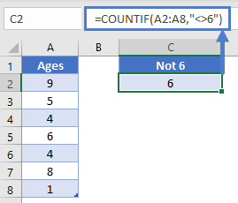

Now we can quickly see that we have 6 kids that are not 6 years old.

In these comparison examples so far, we’ve been hard coding the values we wanted. You can also use a cell reference. The trick is that you need to concatenate the comparison operator with the cell reference. Let’s say that we put the number 7 in cell C2, and we want our formula in D2 to show how many kids are less than 7 years old.

Our formula in D2 needs to look like this:

=COUNTIF(A2:A8, "<"&C2)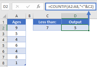

Note: Pay special attention when writing these formulas to whether you need to put an item inside quotation marks, or outside. The operators are always inside quotations, cell references are always outside quotations. Numbers are outside if you’re doing an exact match, but inside if doing a comparison operator.

Working with dates

We’ve seen how you can give a text or number as a criteria, but what about when we need to work with dates? Here’s a quick sample list we can work with:

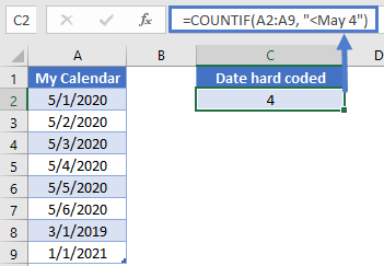
To count how many dates are after May 4, we need to take some caution. Computers store dates as numbers, so we need to make sure the computer uses the right number. If we wrote this formula, would we get the correct result?

=COUNTIF(A2:A9, "<May 4")

The answer is “possibly”. Because we omitted the year from our criteria, the computer will assume we mean the current year. If all the dates we are working with are for the current year, then we’ll get the correct answer. If there are some dates that are in the future however, we’d get the wrong answer. Also, once the next year begins, this formula will return a different result. As such, this syntax should probably be avoided.

Because it can be difficult to write dates correctly within a formula, it’s best practice to write the date you want to use in a cell, and then you can use that cell reference within your COUNTIF formula. So, let’s write the date of 7-May-2020 into cell C2, and then we can put our formula in C4.

The formula in C4 is

=COUNTIF(A2:A9, "<"&C2)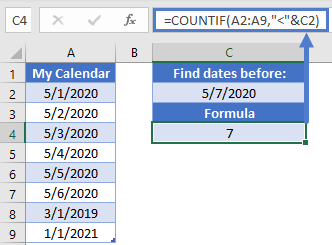

Now we know that the result of 7 is correct, and the answer is not going to change unexpectedly if we open this spreadsheet sometime in the future.

Before we leave this section, it’s common to use the TODAY function when working with dates. We can use that just like we would a cell reference. For instance, we could change the previous formula to be this:

=COUNTIF(A2:A9, "<"&TODAY())

Now our formula will still update as real time progresses, and we will have a count of items that are less than today.

Multiple criteria and COUNTIFS

The original COUNTIF function got an improvement in 2007 when COUNTIFS came out. The syntax between the two is very similar, with the latter allowing you to give additional ranges and criteria. You can easily use COUNTIFS in any situation that COUNTIF exists. It is just a good idea to know that both functions exist.

Let’s look at this table of data:

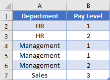
To find out how many people are in pay levels 1 to 2, you could write a summation of COUNTIF functions like this:

=COUNTIF(B2:B7, ">=1")-COUNTIF(B2:B7, ">2")

This formula will work, as you’re finding everything that is above 1, but then subtracting the number of records that are beyond your cut-off point. Alternatively, you could use COUNTIFS like this:

=COUNTIFS(B2:B7, ">=1", B2:B7, "<=2")

The latter is more intuitive to read, so you might want to use that route. Also, COUNTIFS is more powerful when you need to consider multiple columns. Let’s say we want to know how many people are in Management and in Pay Level 1. You can’t do that with just a COUNTIF; you’d need to write out

=COUNTIFS(A2:A7, "Management", B2:B7, 1)

This formula would give you the correct result of 2. Before we leave this section, let’s consider an Or type logic. What if we wanted to find out how many people are in Management or? You would need to add some COUNTIFS together, but there are two ways to do this. The simpler way is to write it like this:

=COUNTIF(A2:A7, "HR")+COUNTIF(A2:A7, "Management")

You could also make use of an array, and write this array formula:

=SUM(COUNTIF(A2:A7, {"HR", "Management"}))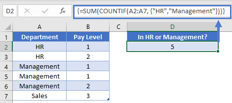

Note: Array formulas must be confirmed using `Ctrl+Shift+Enter` not just `Enter`.

How this formula will work is it will see that you have given an array as the input. It will thus calculate the result to two different COUNTIF functions and store them in an array. The SUM function will then add all the results in our array together to make a single output. Thus, our formula will be evaluated like so:

=SUM(COUNTIF(A2:A7, {"HR", "Management"}))
=SUM({2, 3})
=5

Count unique values

Now that we’ve seen how to use an array with the COUNTIF function, we can take that one step further to help us count how many unique values are in a range. First, let’s look again at our list of Departments.

=SUM(1/COUNTIF(A2:A7,A2:A7))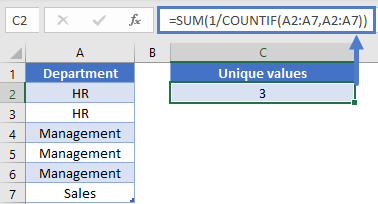

We can see that there are 6 cells worth of data, but there are only 3 different items. To get the math to work out, we’d need each item to be worth 1/N, where N is the number of times an item is repeated. For example, if each HR was only worth 1/2, then when you added them up you would get a count of 1, for 1 unique value.

Back to our COUNTIF, which is designed to figure out how many times an item appears in a range. In D2, we’ll write the array formula

=SUM(1/COUNTIF(A2:A7, A2:A7))

How this formula will work, is for each cell in the range of A2:A7, it will check to see how many times it appears. With our sample, this is going to produce an array of

{2, 2, 3, 3, 3, 1}

Then, we turn all those numbers into fractions by doing some division. Now our array looks like

{1/2, 1/2, 1/3, 1/3, 1/3, 1/1}

When we add these all up, we get our desired result of 3.

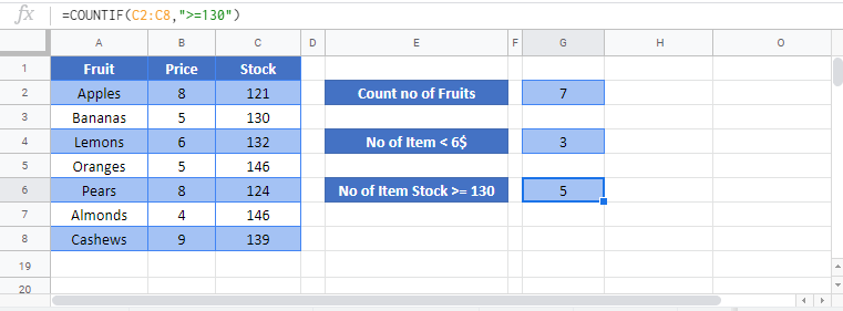
Countif with Two or Multiple Conditions – The Countifs Function

So far we’ve worked only with the COUNTIF Function. The COUNTIF Function can only handle one criteria at a time. To COUNTIF with multiple criteria you need to use the COUNTIFS Function. COUNTIFS behaves exactly like COUNTIF. You just add extra criteria. Let’s take a look at below example.

=COUNTIFS(B2:B7,"<6",C2:C7,">=130")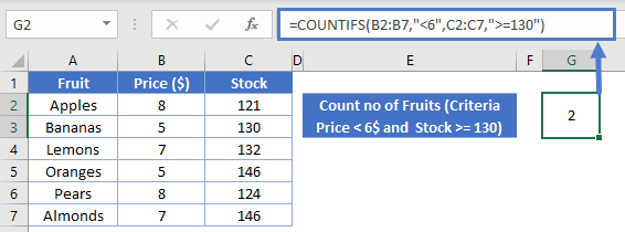

COUNTIF & COUNTIFS in Google Sheets

The COUNTIF & COUNTIFS Function works exactly the same in Google Sheets as in Excel: