
Excel for Microsoft 365 Excel 2021 Excel 2019 Excel 2016 Excel 2013 Excel 2010 Excel 2007 More…Less
To count numbers or dates that meet a single condition (such as equal to, greater than, less than, greater than or equal to, or less than or equal to), use the COUNTIF function. To count numbers or dates that fall within a range (such as greater than 9000 and at the same time less than 22500), you can use the COUNTIFS function. Alternately, you can use SUMPRODUCT too.
Example
Note: You’ll need to adjust these cell formula references outlined here based on where and how you copy these examples into the Excel sheet.
|
1 |
A |
B |
|---|---|---|
|
2 |
Salesperson |
Invoice |
|
3 |
Buchanan |
15,000 |
|
4 |
Buchanan |
9,000 |
|
5 |
Suyama |
8,000 |
|
6 |
Suyma |
20,000 |
|
7 |
Buchanan |
5,000 |
|
8 |
Dodsworth |
22,500 |
|
9 |
Formula |
Description (Result) |
|
10 |
=COUNTIF(B2:B7,»>9000″) |
The COUNTIF function counts the number of cells in the range B2:B7 that contain numbers greater than 9000 (4) |
|
11 |
=COUNTIF(B2:B7,»<=9000″) |
The COUNTIF function counts the number of cells in the range B2:B7 that contain numbers less than 9000 (4) |
|
12 |
=COUNTIFS(B2:B7,»>=9000″,B2:B7,»<=22500″) |
The COUNTIFS function (available in Excel 2007 and later) counts the number of cells in the range B2:B7 greater than or equal to 9000 and are less than or equal to 22500 (4) |
|
13 |
=SUMPRODUCT((B2:B7>=9000)*(B2:B7<=22500)) |
The SUMPRODUCT function counts the number of cells in the range B2:B7 that contain numbers greater than or equal to 9000 and less than or equal to 22500 (4). You can use this function in Excel 2003 and earlier, where COUNTIFS is not available. |
|
14 |
Date |
|
|
15 |
3/11/2011 |
|
|
16 |
1/1/2010 |
|
|
17 |
12/31/2010 |
|
|
18 |
6/30/2010 |
|
|
19 |
Formula |
Description (Result) |
|
20 |
=COUNTIF(B14:B17,»>3/1/2010″) |
Counts the number of cells in the range B14:B17 with a data greater than 3/1/2010 (3) |
|
21 |
=COUNTIF(B14:B17,»12/31/2010″) |
Counts the number of cells in the range B14:B17 equal to 12/31/2010 (1). The equal sign is not needed in the criteria, so it is not included here (the formula will work with an equal sign if you do include it («=12/31/2010»). |
|
22 |
=COUNTIFS(B14:B17,»>=1/1/2010″,B14:B17,»<=12/31/2010″) |
Counts the number of cells in the range B14:B17 that are between (inclusive) 1/1/2010 and 12/31/2010 (3). |
|
23 |
=SUMPRODUCT((B14:B17>=DATEVALUE(«1/1/2010»))*(B14:B17<=DATEVALUE(«12/31/2010»))) |
Counts the number of cells in the range B14:B17 that are between (inclusive) 1/1/2010 and 12/31/2010 (3). This example serves as a substitute for the COUNTIFS function that was introduced in Excel 2007. The DATEVALUE function converts the dates to a numeric value, which the SUMPRODUCT function can then work with. |
Need more help?
Want more options?
Explore subscription benefits, browse training courses, learn how to secure your device, and more.
Communities help you ask and answer questions, give feedback, and hear from experts with rich knowledge.
Home / Excel Formulas / Count Between Two Numbers (COUNTIFS)
In Excel, you can count between two numbers using the COUNTIFS function. With the COUNTIFS function, you can specify an upper limit of the numbers, and a lower limit to create a range of numbers to count. In the following example, we have a list of names with age. Now we need to count the people of two ages i.e., two numbers.
sample-file

You can use the following steps to create formulas using the COUNTIFS to count numbers between 10 and 25.
- First, enter the “=COUNTIS(“ in cell C1.

- After that, refer to the range from where you want to count the values.

- Next, you need to specify the upper number using greater than and equal sign.

- From here, again you need to refer to the range of numbers in the criteria2.

- In the end, use lower than and equal signs to specify number below than 10 in the counting range.


=COUNTIFS(B2:B26,"<=25",B2:B26,">=10")COUNTIFS can take multiple criteria and count values based on them, and to understand this formula, we need to split it into two parts.

- First, you have specified the range from which you want to count the numbers and the upper number using the greater than and equal signs.
- After that, you specified the lower number and the range of numbers.
sample-file
Using SUMPRODUCT to Count Cells Between Two Numbers
You can also use the SUMPRODUCT function for counting the number of cells between two numbers. In this formula, we need to use the INT function along with the SUMPRODUCT. See the formula below:
=SUMPRODUCT(INT(B2:B26>=10), INT(B2:B26<=25))
To understand the formula, we need to split it:
In the first INT function, we have used the range of cells from where we want to count the numbers. And >= signs to only refer to the numbers greater than or equal to 10. And it returns an array showing all the numbers above 10 using 1.

And in the second INT function, again you have the same range that considers the numbers lower than and equal to 25.

With both INT functions, you have two different arrays. In the first, you have 1 for each number that is greater than or equal to 10, and in the second, 1 for the values which are lower than or equal to 25.

In the end,
- SUMPRODUCT multiplies each value from the first array with the value from the second array, and you will get an array of values that represents numbers that are between 10 and 25.
- And after that return the sum of those values from the array.
sample-file
In this example, the goal is to count numbers that fall within specific ranges. The lower value comes from the «Start» column, and the upper value comes from the «End» column. For each range, we want to include both the lower value and the upper value. For convenience, the numbers being counted are in the named range data (C5:C16). This problem can be solved with both the COUNTIFS function and the SUMPRODUCT function, as explained below.
COUNTIFS function
In the example shown, the formula used to solve this problem is based on the COUNTIFS function, which is designed to count cells that meet multiple criteria. The formula in cell G5, copied down, is:
=COUNTIFS(data,">="&E5,data,"<="&F5)
COUNTIFS accepts criteria in range/criteria pairs. The first range/criteria pair checks for values in data that are greater than or equal to (>=) the «Start» value in column E:
data,">="&E5
The second range/criteria pair checks for values in data that are less than or equal to (<=) the «End» value in column F:
data,"<="&F5
Because we supply the same range (data) for both criteria, each cell in data must meet both conditions in order to be included in the final count. Note in both cases, we need to concatenate the cell reference to the logical operator. This is a quirk of RACON functions in Excel, which use a different syntax than other formulas.
As the formula is copied down column G, it returns the count of numbers that fall in the range defined by columns E and F.
SUMPRODUCT alternative
Another option for solving this problem is the SUMPRODUCT function with a formula like this:
=SUMPRODUCT((data>=E5)*(data<=F5))
This is an example of using Boolean logic. Because there are 12 values in the named range data, each logical expression inside SUMPRODUCT generates an array that contains 12 TRUE and FALSE values. The expression:
data>=E5
returns:
{TRUE;TRUE;TRUE;TRUE;TRUE;TRUE;TRUE;TRUE;TRUE;TRUE;TRUE;TRUE}
And the expression:
data<=F5
returns:
{TRUE;FALSE;FALSE;FALSE;TRUE;FALSE;FALSE;FALSE;TRUE;FALSE;TRUE;FALSE}
When these two arrays are multiplied together, the math operation causes TRUE values to be coerced to 1 and FALSE values to be coerced to zero. The result is a single array of 1s and 0s like this:
=SUMPRODUCT({1;0;0;0;1;0;0;0;1;0;1;0})
Each 1 corresponds to a number in data that meets both conditions and each 0 represents a number that fails at least one condition. With only a single array to process, SUMPRODUCT returns the sum of the numbers in the array, 4, as a final result.
Video: Boolean logic in Excel
Benefits of standard syntax
The nice thing about SUMPRODUCT is that it will handle array operations natively (no need to enter with control + shift + enter) and will accept the more standard syntax for logical expressions seen above. The standard syntax is more useful in other modern formulas. For example you could use the same exact logic with the FILTER function to return the actual numbers that meet these same conditions:
=FILTER(data,(data>=E5)*(data<=F5))
Becomes:
=FILTER(data,{1;0;0;0;1;0;0;0;1;0;1;0})
And FILTER returns the numbers greater than or equal to 70 and less than or equal to 79:
{79;77;75;70}
Video: Basic FILTER function example
Using the COUNTIFS function you can achieve the result of counting numbers of cells which contain values between two numbers in a range.
Using the COUNTIFS Function Between Two Values
The COUNTIFS function can show the count of cells that meet your criteria. You can use COUNTIF with criteria using dates, numbers, text and other conditions.
Using COUNTIFS you also need to use logical operators (>,<,<>,=).
The COUNTIFS function is built to count cells that meet multiple criteria. In this case, because we supply the same range for two criteria, each cell in the range must meet both criteria in order to be counted.
Generic formula :
=COUNTIFS(range,">=X",range,"<=Y")
Use >= for greater than or equal to
Use <= for less than or equal to
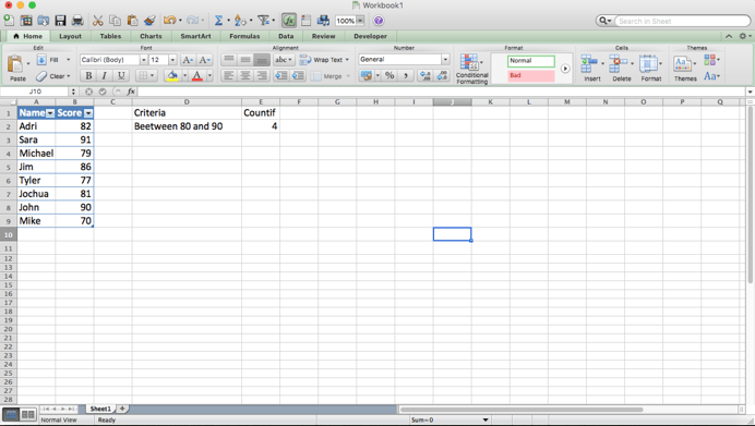
So if we want to count based on criteria : Between 80 and 90 in our table, we use this formula :
=COUNTIFS(B2:B9,">=80",B2:B9,"<=90") and the result should be 4 ( including : 82, 86, 81 and 90 )
Using COUNTIFS between dates
The following COUNTIFS formula shows this idea by counting the number of dates that fall between a start and end date. The following formula counts the number of dates in A2:A9 that are equal to or greater than the date in E1 and equal to or less than the date in E2:
To count the number of cells that contain dates between two dates, you can use the COUNTIFS function:
=COUNTIFS(range,">="&date1,range,"<="&date2)
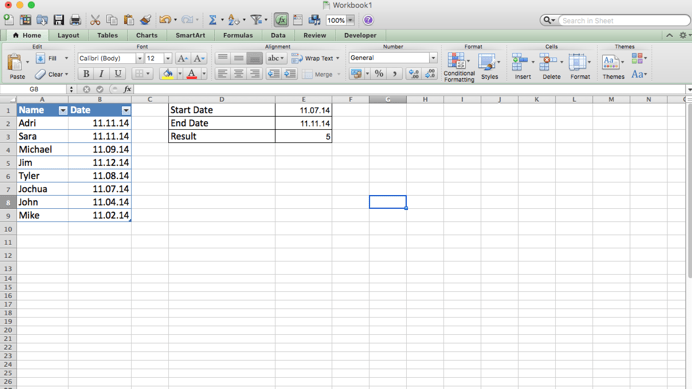
=COUNTIFS($B$2:$B$9,">="&$E$1,$B$2:$B$9,"<="&$E$2)
So dates between 11/07/14 and 11/11/14 are found 5 dates, from B2 cell to B7 cell.
The COUNTIFS formula with multiple criteria
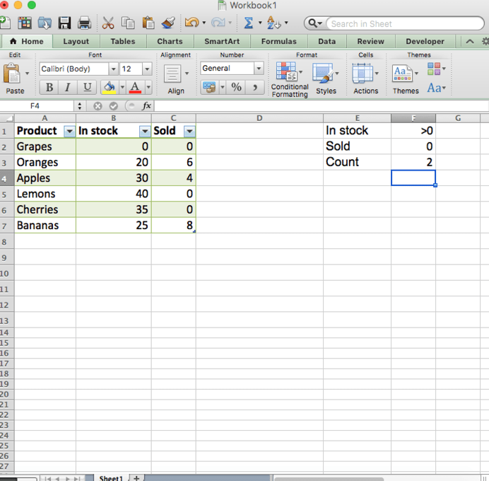
Suppose you have a product list like in the example below, and you want to get a count of items that are in stock (value in column B is greater than 0) but have not been sold yet (value in column C is equal to 0).
The task can be accomplished by using this formula:
=COUNTIFS(B2:B7,">0", C2:C7,"=0")
And the count is 2 (“Cherries” and “Lemons”)
When you want to count items with identical criteria, you still need to supply each criteria_range / criteria pair individually.
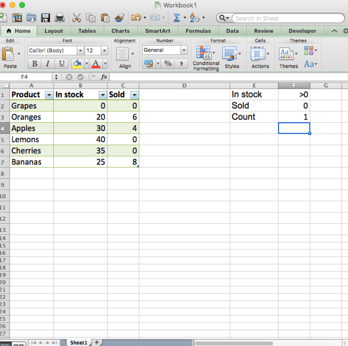
For example, here’s the right formula to count items that have 0 both in column B and column C:
=COUNTIFS($B$2:$B$7,"=0", $C$2:$C$7,"=0")
This COUNTIFS formula returns 1 because only “Grapes” have “0” value in both columns.
Different problems have their own best solution. If you are stuck and want to get to the solution quick, ask your question to have it answered by an Excel expert in 20 minutes. They are available to help you 24/7 at the link to the right. The first question is free.
MS Excel is the top source to compute different values and analyze tons of data. When it comes to counting values added in the cells, Excel tends to have multiple functions. Your data may include text values, numbers, dates, characters, or anything else. Here you will get to know how to CountIf between two numbers or values.
Before proceeding, let’s have a look at what this function is and how it works.
What is COUNTIF Function and How does it Work?
Excel users must have an idea about the COUNTIF function that is used to count numbers of different cells including values. With the help of a formula, you can easily count the number of a cell having different values between two numbers. These values could be in a specific range of cells or columns. You may use it with two COUNTIF functions given in the same value.
As you already know, this function is made to count cells and for two different criteria, all cells in the given range have to be compatible with both criteria to be in the function.
Generic Formula
=COUNTIFs(range,”>=smallest_num”,range,”<=largest_num”)
Let’s know about Arguments:
range: A range has values that count the number of cells that exists between two values.
smallest_num: It is the smallest number that counts the cells.
largest_num: It is the largest number that counts the cells.
Explanation
Using this formula lets you help in counting the number of cells that consist of values between two numbers.
How to Use CountIf Between Two Numbers
With an example, you will easily understand the formula. Let’s use a small subtract logic with the COUNTIF function.
At first, it helps in counting each number bigger than 50. Suppose in the list we have numbers such as 85, 75, 60, 55, 46, 62, 67, 28, 45, 30. It simply means that 6 numbers are bigger than 50 which simply explains the functioning of the first part of the formula.
=COUNTIF(B2:B11,”>=50”)
Furthermore, in the second step, we will have to count all the numbers bigger than 80 while subtracting them from the first count. In this list, we found just 1 figure bigger than 80, which is 85.
-COUNTIF(B2:B11,”>80”)
In a nutshell, 6-1=5, and that’s what we are supposed to have. Let’s assume, you want to count the number of students who scored between 50 to 80. While putting the figures in the formula, let’s have a look at it.
The complete formula will appear like this:
=COUNTIF(B2:B11,”>=50”)-COUNTIF(B2:B11,”>80)
Rather than applying a particular range of cells, you may want to count the whole column. In that case, your formula will appear like this:
=COUNTIF(B:B,”>=50”)-COUNTIF(B:B,”>80”)
In case, if you need to choose the first, ending, or between numbers given in different cells, you should try applying them right in the formula. And the formula will appear like this:
=COUNTIF(B2:B11,”>”&E1)-COUNTIF(B2:B11,”>”&F1)
Do you get an idea of how to use COUNTIF between two numbers while using Excel?
You must have come to know how simple and easy this function is. Let’s dig out more to understand this function naturally.
How to Count Cells within a Range using COUNTIF
In this section, we will use the COUNTIF formula to count a range of cells. In the figure below, you can find the data given in which we will tend to find the number of sales when the targeted sales value comes up between $150 and $500.

- In cell E4, you have to apply the formula and press Enter key from the keyboard.
=COUNTIF(C4:C12,”>”&D4)-COUNTIF(C4:C12,”>”&D5)

How to Count Cells by Comparing Numbers and Dates with COUNTIF
In this section, you will get to know how to compare the cells with the COUNTIF function. Suppose that we are having a dataset containing Salespersons and the Sales together with the Sales Target Amount. Now, you need to count the cells having the same or bigger value than the Criteria Sales value.

- In cell E4, you need to add the Formula.
=COUNTIF(C4:C12,”>=”&D4)

- Once you press the Enter key, the result will appear on the screen.

This is how you can compare numbers between two cells with COUNTIF function.
Enter the Formula for OR Function with COUNTIF
Here, you will see how to find a unique or a duplicate value with the help of the COUNTIF function. Suppose we have a dataset of employees with their ID. Let’s operate the formula on this given dataset.

- In cell D4, you have to enter the formula and press Enter key.
=SUMPRODUCT ((COUNTIF(B4:B17, B4:B17)>1)*(B4:B17<>””))

- You need to repeat the procedure for finding the unique values. In cell E4, enter the formula and press Enter key.
=SUMPRODUCT ((COUNTIF(B4:B17,B4:B17)=1)*(B4:B17<>””))

This is how you can find duplicates of unique values.
How to Count a Particular Time with COUNTIF
In this part of the post, you will see another great usage of the COUNTIF function. Suppose that in the dataset we have a person John having a daily cycling duration. And the duration format appears in hh:mm:ss, which is hours, minutes, and then seconds sequentially. Let’s see how to count the cell greater than or equal to the value in cell D4.

- In the cell, E4 add the formula and press the Enter key from the keyboard.
=COUNTIF(C4:C12,”>=”&D4)

To Sum Up
That’s it. Some of the handy ways that help you COUNTIF between two numbers are mentioned above. You can try any of them and hopefully, you will find them effective. Each method is explained with examples that make your understanding easier. Keep practicing these methods and continue sharing them with your friends.