
Return to Excel Formulas List
Download Example Workbook
Download the example workbook
This tutorial will demonstrate how to count cells that do not contain specific text.
Count Cells that Do Not Contain Specific Text with COUNTIF
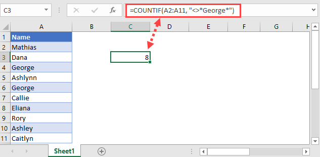
The COUNTIF Function counts all cells that meet a certain condition. We can use the COUNTIF Function along with the not equal to sign, <>, and the asterisk wildcard, *, to count cells that do not contain certain text.
In this example, we will count all cells that do not contain the text “Ash”:
=COUNTIF(A2:A11,"<>*Ash*")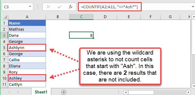
As highlighted above, since the cells A5 and A10 start with the word “Ash”, they are not counted.
Count Cells that Do Not Contain Specific Text with COUNTIF in Google Sheets
These functions also work the same way in Google Sheets as well.
=COUNTIF(Range, “<>*Ash*”)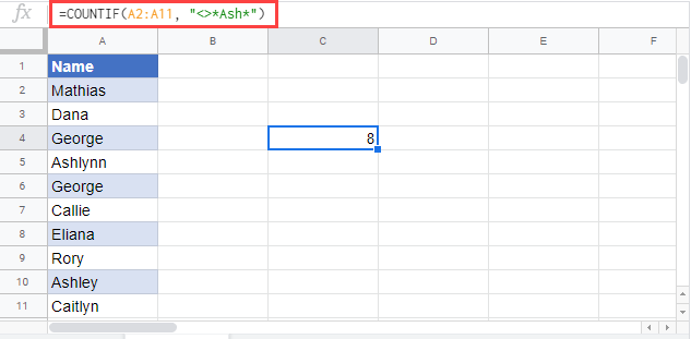
In this example, the goal is to count cells that do not contain a specific substring. This problem can be solved with the COUNTIF function or the SUMPRODUCT function. Both approaches are explained below. Although COUNTIF is not case-sensitive, the SUMPRODUCT version of the formula can be adapted to perform a case-sensitive count. For convenience, data is the named range B5:B15.
COUNTIF function
The COUNTIF function counts cells in a range that meet supplied criteria. For example, to count the number of cells in a range that contain «apple» you can use COUNTIF like this:
=COUNTIF(range,"apple") // equal to "apple"
Note this is an exact match. To be included in the count, a cell must contain «apple» and only «apple». If a cell contains any other characters, it will not be counted. To reverse this operation and count cells that do not contain «apple», you can add the not equal to (<>) operator like this:
=COUNTIF(range,"<>apple") // not equal to "apple"
The goal in this example is to count cells that do not contain specific text, where the text is a substring that can be anywhere in the cell. To do this, we need to use the asterisk (*) character as a wildcard. To count cells that contain the substring «apple», we can use a formula like this:
=COUNTIF(range,"*apple*") // contains "apple"
The asterisk (*) wildcard matches zero or more characters of any kind, so this formula will count cells that contain «apple» anywhere in the cell. To count cells that do not contain the substring «apple», we add the not equal to (<>) operator like this:
=COUNTIF(range,"<>*apple*") // does not contain "apple"
The formulas used in the worksheet shown follow the same pattern:
=COUNTIF(data,"<>*a*") // does not contain "a"
=COUNTIF(data,"<>*0*") // does not contain "0"
=COUNTIF(data,"<>*-r*") // does not contain "-r"
Data is the named range B5:B15. The COUNTIF function supports three different wildcards, see this page for more details.
Note the COUNTIF formula above won’t work if you are targeting a particular number and cells contain numeric data. This is because the wildcard automatically causes COUNTIF to look for text only (i.e. to look for «2» instead of just 2). In addition, COUNTIF is not case-sensitive, so you can’t perform a case-sensitive count. The SUMPRODUCT alternative explained below can handle both situations.
With a cell reference
You can easily adjust this formula to use a cell reference in criteria. For example, if A1 contains the substring you want to exclude from the count, you can use a formula like this:
=COUNTIF(range,"<>*"&A1&"*")
Inside COUNTIF, the two asterisks and the not equal to operator (<>) are concatenated to the value in A1, and the formula works as before.
Exclude blanks
To exclude blank cells, you can switch to COUNTIFS function and add another condition like this:
=COUNTIFS(range,"<>*a*",range,"?*") // requires some text
The second condition means «at least one character».
See also: 50 examples of formula criteria
SUMPRODUCT function
Another way to solve this problem is with the SUMPRODUCT function and Boolean algebra. This approach has the benefit of being case-sensitive if needed. In addition, you can use this technique to target a number inside of a number, something you can’t do with COUNTIF.
To count cells that contain specific text with SUMPRODUCT, you can use the SEARCH function. SEARCH returns the position of text in a text string as a number. For example, the formula below returns 6 since the «a» appears first as the sixth character in the string:
=SEARCH( "a","The cat sat") // returns 6
If the text is not found, SEARCH returns a #VALUE! error:
=SEARCH( "x","The cat sat") // returns #VALUE!
Notice we do not need to use any wildcards because SEARCH will automatically find substrings. If we get a number from SEARCH, we know the substring was found. If we get an error, we know the substring was not found. This means we can add the ISNUMBER function to evaluate the result from SEARCH like this:
=ISNUMBER(SEARCH( "a","The cat sat")) // returns TRUE
=ISNUMBER(SEARCH( "x","The cat sat")) // returns FALSE
To reverse the operation, we add the NOT function:
=NOT(ISNUMBER(SEARCH( "a","The cat sat"))) // FALSE
=NOT(ISNUMBER(SEARCH( "x","The cat sat"))) // TRUE
We now have what we need to count cells that do not contain a substring with SUMPRODUCT. Back in the example worksheet, to count cells that do not contain «a» with SUMPRODUCT, you can use a formula like this
=SUMPRODUCT(--NOT(ISNUMBER(SEARCH("a",data))))
Working from the inside out, SEARCH is configured to look for «a»:
SEARCH("a",data)
Because data (B5:B15) contains 11 cells, the result from SEARCH is an array with 11 results:
{1;1;1;1;2;2;#VALUE!;#VALUE!;#VALUE!;#VALUE!;#VALUE!}
In this array, numbers indicate the position of «a» in cells where «a» is found. The #VALUE! errors indicate cells where «a» was not found. To convert these results into a simple array of TRUE and FALSE values, we use the ISNUMBER function:
ISNUMBER(SEARCH("a",data))
ISNUMBER returns TRUE for any number and FALSE for errors. SEARCH delivers the array of results to ISNUMBER, and ISNUMBER converts the results to an array that contains only TRUE and FALSE values:
{TRUE;TRUE;TRUE;TRUE;TRUE;TRUE;FALSE;FALSE;FALSE;FALSE;FALSE}
In this array, TRUE corresponds to cells that contain «a» and FALSE corresponds to cells that do not contain «a». This is exactly the opposite of what we need, so we use the NOT function to reverse the array:
NOT(ISNUMBER(SEARCH("a",data)))
The result from the NOT function is:
{FALSE;FALSE;FALSE;FALSE;FALSE;FALSE;TRUE;TRUE;TRUE;TRUE;TRUE}
In this array, the TRUE values represent cells we want to count. However, we first need to convert the TRUE and FALSE values to their numeric equivalents, 1 and 0. To do this, we use a double negative (—):
--NOT(ISNUMBER(SEARCH("a",data)))
The result inside of SUMPRODUCT looks like this:
=SUMPRODUCT({0;0;0;0;0;0;1;1;1;1;1}) // returns 5
With a single array to process, SUMPRODUCT sums the array and returns 5 as a final result.
One benefit of this formula is it will find a number inside a numeric value. In addition, there is no need to use wildcards to indicate position, because SEARCH will automatically look through all text in a cell.
Case-sensitive option
For a case-sensitive count, you can replace the SEARCH function with the FIND function like this:
=SUMPRODUCT(--NOT(ISNUMBER(FIND("A",data))))
The FIND function works just like the SEARCH function, but is case-sensitive. Notice we have replaced «a» with «A» because FIND is case-sensitive. If we used «a», the result would be 11 since there are no cells in B5:B15 that contain a lowercase «a». This example provides more detail.
Note: the SUMPRODUCT formulas above are more complex, but using Boolean operations in array formulas is a more powerful and flexible approach. It is also an important skill in modern functions like FILTER and XLOOKUP, which often use this technique to select the right data. The syntax used by COUNTIF is unique to a group of eight functions and is therefore not as useful or portable.
In the previous post, we talked that how to count cell that contain certain text using the COUNTIF function in Excel.
This post will guide you how to count the number of cells that do not contain specific text within a range of cells using a formula in Excel 2013/2016 or Excel 365. How do I count the number of cells without certain text using a simple formula in Excel. When you analyze a large list of data, you may also want to know that how many cells that do not contain specific text. The below steps will show you how to do it in a simple way.
Table of Contents
- 1. Count Number of Cells that do Not Contain Specific Text Using COUNTIF Function
- 2. Count Number of Cells that do Not Contain Specific Text With VBA Code
- 3. Video: Count Number of Cells that do Not Contain Specific Text
- 4. Related Functions
1. Count Number of Cells that do Not Contain Specific Text Using COUNTIF Function
You can use the COUNTIF function to count cells that do not contain certain text. And you also need to supply the target text string in the criteria argument in the COUNTIF function.
The below is a generic formula to count the number of cells that do not contain specific text:
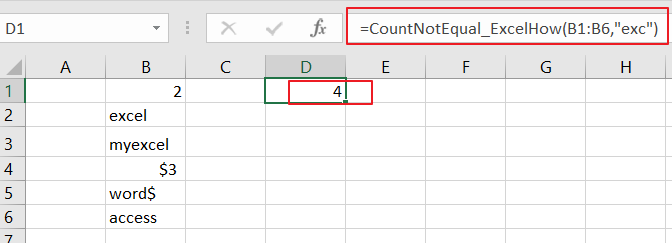
=COUNTIF(range,criteria)Assuming that you have a list of data in range B1:B6 and you want to count the number of cells without a certain text “exc”. And you can type this string in the second argument as its criteria and you will get the below formula:
=COUNTIF(B1:B6,"<>*exc*")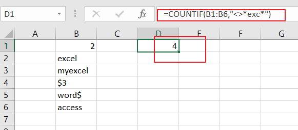
LET’S SEE THAT HOW THIS FORMULA WORKS:
The COUNTIF function can be used to count the number of cells that match a single condition or criteria. And in this case, you need to provide a criteria as “<>*exc*”, which is evaluated as “values that do not contain ‘exc’ in any position”. Then the total count of all cells in the range B1:B6 that meet the above criteria is returned.
The “<>” operator means that does not equal to a certain value, so the above formula can be used to count any cell that does not contain “exc” in any position in cells.
2. Count Number of Cells that do Not Contain Specific Text With VBA Code
You can also use a User-defined function with VBA code to count number of cells that do not contain a specific text string in Excel, just do the following steps:
Step1: Press Alt + F11 to open the Visual Basic Editor.
![]()
Step2: In the Visual Basic Editor, click on Insert > Module.
![]()
Step3: In the new module, enter the following code:
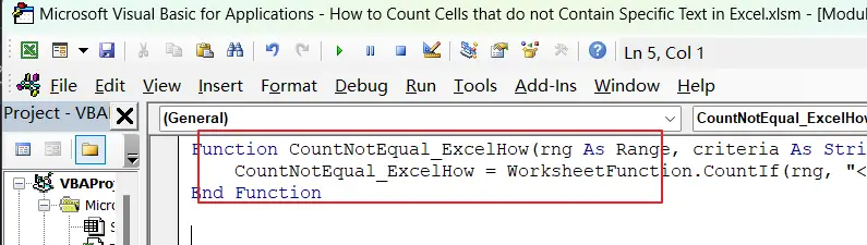
Function CountNotEqual_ExcelHow(rng As Range, criteria As String) As Long
    CountNotEqual_ExcelHow = WorksheetFunction.CountIf(rng, "<>*" & criteria & "*")
End Function
Step4: Save the module with a suitable name, such as “CountNotEqual_ExcelHow“. And return to your worksheet, and enter a cell where you want to use the user-defined function.
Step5: In any blank cell, enter the formula:
=CountNotEqual_ExcelHow(B1:B6,"exc")Where ” B1:B6” is the range you want to count and “exc” is the specific text you want to exclude.
Step6: Press Enter, and the formula will return the count of cells that do not contain the specific text.
3. Video: Count Number of Cells that do Not Contain Specific Text
This video will demonstrate two methods to count cells that do not contain specific text in Excel – using the COUNTIF function and VBA code.
- Excel COUNTIF function
The Excel COUNTIF function will count the number of cells in a range that meet a given criteria. This function can be used to count the different kinds of cells with number, date, text values, blank, non-blanks, or containing specific characters. etc. = COUNTIF (range, criteria) …
When writing content on nearly all text editors be it Microsoft Word, PowerPoint, or even excel, there are these options to search or rather find and replace located on the Home tab. This function will search and find the specific text that you just wanted to find.
Microsoft Excel is one of the text editors, also has that capability. You find that in a given excel sheet several cells are containing specific values depending on the data that was fed on it. Since in this scenario we are not interested in finding the specific text, we do not need to bear with the noting of all specific letters.
Counting is the act of tallying a certain quantity to obtain or to reveal the number of items or several objects in a set. We count to get tall in numerical values. Counting is general and done in almost all aspects of life or our daily routines.
There are some of the ways to follow to do a quick tally of cells that do not contain specific text in an excel sheet. Some of the steps involved include;
Step 1
Open a blank excel sheet and insert some data into it, you can have one column with student and the other with weights. The data may look like the one below.

Step 2
This is the step in that we wish to establish the count of the cells that do not contain specific text. To get tall, there are a couple of things we need to do first; we need to know the formula, how to use it, and where to write it. Select an empty cell.

Counting cells that do not have specific text will involve the use of the function COUNTIF. This function does the tally if a certain condition is met or achieved. We use the function in the formula in this format =COUNTIF (A2: A5,»<>*count*»).

In the above formula, COUNTIF is the function to calculate the values, A2 and A5 are the number of cells in the range and finally, the count is the condition in this case.

The count of cells that do not contain specific text in the above case is 4.
COUNTIF function
Use COUNTIF, one of the statistical functions, to count the number of cells that meet a criterion; for example, to count the number of times a particular city appears in a customer list.
In its simplest form, COUNTIF says:
-
=COUNTIF(Where do you want to look?, What do you want to look for?)
For example:
-
=COUNTIF(A2:A5,»London»)
-
=COUNTIF(A2:A5,A4)

COUNTIF(range, criteria)
|
Argument name |
Description |
|---|---|
|
range (required) |
The group of cells you want to count. Range can contain numbers, arrays, a named range, or references that contain numbers. Blank and text values are ignored. Learn how to select ranges in a worksheet. |
|
criteria (required) |
A number, expression, cell reference, or text string that determines which cells will be counted. For example, you can use a number like 32, a comparison like «>32», a cell like B4, or a word like «apples». COUNTIF uses only a single criteria. Use COUNTIFS if you want to use multiple criteria. |
Examples
To use these examples in Excel, copy the data in the table below, and paste it in cell A1 of a new worksheet.
|
Data |
Data |
|---|---|
|
apples |
32 |
|
oranges |
54 |
|
peaches |
75 |
|
apples |
86 |
|
Formula |
Description |
|
=COUNTIF(A2:A5,»apples») |
Counts the number of cells with apples in cells A2 through A5. The result is 2. |
|
=COUNTIF(A2:A5,A4) |
Counts the number of cells with peaches (the value in A4) in cells A2 through A5. The result is 1. |
|
=COUNTIF(A2:A5,A2)+COUNTIF(A2:A5,A3) |
Counts the number of apples (the value in A2), and oranges (the value in A3) in cells A2 through A5. The result is 3. This formula uses COUNTIF twice to specify multiple criteria, one criteria per expression. You could also use the COUNTIFS function. |
|
=COUNTIF(B2:B5,»>55″) |
Counts the number of cells with a value greater than 55 in cells B2 through B5. The result is 2. |
|
=COUNTIF(B2:B5,»<>»&B4) |
Counts the number of cells with a value not equal to 75 in cells B2 through B5. The ampersand (&) merges the comparison operator for not equal to (<>) and the value in B4 to read =COUNTIF(B2:B5,»<>75″). The result is 3. |
|
=COUNTIF(B2:B5,»>=32″)-COUNTIF(B2:B5,»<=85″) |
Counts the number of cells with a value greater than (>) or equal to (=) 32 and less than (<) or equal to (=) 85 in cells B2 through B5. The result is 1. |
|
=COUNTIF(A2:A5,»*») |
Counts the number of cells containing any text in cells A2 through A5. The asterisk (*) is used as the wildcard character to match any character. The result is 4. |
|
=COUNTIF(A2:A5,»?????es») |
Counts the number of cells that have exactly 7 characters, and end with the letters «es» in cells A2 through A5. The question mark (?) is used as the wildcard character to match individual characters. The result is 2. |
Common Problems
|
Problem |
What went wrong |
|---|---|
|
Wrong value returned for long strings. |
The COUNTIF function returns incorrect results when you use it to match strings longer than 255 characters. To match strings longer than 255 characters, use the CONCATENATE function or the concatenate operator &. For example, =COUNTIF(A2:A5,»long string»&»another long string»). |
|
No value returned when you expect a value. |
Be sure to enclose the criteria argument in quotes. |
|
A COUNTIF formula receives a #VALUE! error when referring to another worksheet. |
This error occurs when the formula that contains the function refers to cells or a range in a closed workbook and the cells are calculated. For this feature to work, the other workbook must be open. |
Best practices
|
Do this |
Why |
|---|---|
|
Be aware that COUNTIF ignores upper and lower case in text strings. |
|
|
Use wildcard characters. |
Wildcard characters —the question mark (?) and asterisk (*)—can be used in criteria. A question mark matches any single character. An asterisk matches any sequence of characters. If you want to find an actual question mark or asterisk, type a tilde (~) in front of the character. For example, =COUNTIF(A2:A5,»apple?») will count all instances of «apple» with a last letter that could vary. |
|
Make sure your data doesn’t contain erroneous characters. |
When counting text values, make sure the data doesn’t contain leading spaces, trailing spaces, inconsistent use of straight and curly quotation marks, or nonprinting characters. In these cases, COUNTIF might return an unexpected value. Try using the CLEAN function or the TRIM function. |
|
For convenience, use named ranges |
COUNTIF supports named ranges in a formula (such as =COUNTIF(fruit,»>=32″)-COUNTIF(fruit,»>85″). The named range can be in the current worksheet, another worksheet in the same workbook, or from a different workbook. To reference from another workbook, that second workbook also must be open. |
Note: The COUNTIF function will not count cells based on cell background or font color. However, Excel supports User-Defined Functions (UDFs) using the Microsoft Visual Basic for Applications (VBA) operations on cells based on background or font color. Here is an example of how you can Count the number of cells with specific cell color by using VBA.
Need more help?
You can always ask an expert in the Excel Tech Community or get support in the Answers community.

See also
COUNTIFS function
IF function
COUNTA function
Overview of formulas in Excel
IFS function
SUMIF function
Need more help?
Want more options?
Explore subscription benefits, browse training courses, learn how to secure your device, and more.
Communities help you ask and answer questions, give feedback, and hear from experts with rich knowledge.