
COUNTIF function
Use COUNTIF, one of the statistical functions, to count the number of cells that meet a criterion; for example, to count the number of times a particular city appears in a customer list.
In its simplest form, COUNTIF says:
-
=COUNTIF(Where do you want to look?, What do you want to look for?)
For example:
-
=COUNTIF(A2:A5,»London»)
-
=COUNTIF(A2:A5,A4)

COUNTIF(range, criteria)
|
Argument name |
Description |
|---|---|
|
range (required) |
The group of cells you want to count. Range can contain numbers, arrays, a named range, or references that contain numbers. Blank and text values are ignored. Learn how to select ranges in a worksheet. |
|
criteria (required) |
A number, expression, cell reference, or text string that determines which cells will be counted. For example, you can use a number like 32, a comparison like «>32», a cell like B4, or a word like «apples». COUNTIF uses only a single criteria. Use COUNTIFS if you want to use multiple criteria. |
Examples
To use these examples in Excel, copy the data in the table below, and paste it in cell A1 of a new worksheet.
|
Data |
Data |
|---|---|
|
apples |
32 |
|
oranges |
54 |
|
peaches |
75 |
|
apples |
86 |
|
Formula |
Description |
|
=COUNTIF(A2:A5,»apples») |
Counts the number of cells with apples in cells A2 through A5. The result is 2. |
|
=COUNTIF(A2:A5,A4) |
Counts the number of cells with peaches (the value in A4) in cells A2 through A5. The result is 1. |
|
=COUNTIF(A2:A5,A2)+COUNTIF(A2:A5,A3) |
Counts the number of apples (the value in A2), and oranges (the value in A3) in cells A2 through A5. The result is 3. This formula uses COUNTIF twice to specify multiple criteria, one criteria per expression. You could also use the COUNTIFS function. |
|
=COUNTIF(B2:B5,»>55″) |
Counts the number of cells with a value greater than 55 in cells B2 through B5. The result is 2. |
|
=COUNTIF(B2:B5,»<>»&B4) |
Counts the number of cells with a value not equal to 75 in cells B2 through B5. The ampersand (&) merges the comparison operator for not equal to (<>) and the value in B4 to read =COUNTIF(B2:B5,»<>75″). The result is 3. |
|
=COUNTIF(B2:B5,»>=32″)-COUNTIF(B2:B5,»<=85″) |
Counts the number of cells with a value greater than (>) or equal to (=) 32 and less than (<) or equal to (=) 85 in cells B2 through B5. The result is 1. |
|
=COUNTIF(A2:A5,»*») |
Counts the number of cells containing any text in cells A2 through A5. The asterisk (*) is used as the wildcard character to match any character. The result is 4. |
|
=COUNTIF(A2:A5,»?????es») |
Counts the number of cells that have exactly 7 characters, and end with the letters «es» in cells A2 through A5. The question mark (?) is used as the wildcard character to match individual characters. The result is 2. |
Common Problems
|
Problem |
What went wrong |
|---|---|
|
Wrong value returned for long strings. |
The COUNTIF function returns incorrect results when you use it to match strings longer than 255 characters. To match strings longer than 255 characters, use the CONCATENATE function or the concatenate operator &. For example, =COUNTIF(A2:A5,»long string»&»another long string»). |
|
No value returned when you expect a value. |
Be sure to enclose the criteria argument in quotes. |
|
A COUNTIF formula receives a #VALUE! error when referring to another worksheet. |
This error occurs when the formula that contains the function refers to cells or a range in a closed workbook and the cells are calculated. For this feature to work, the other workbook must be open. |
Best practices
|
Do this |
Why |
|---|---|
|
Be aware that COUNTIF ignores upper and lower case in text strings. |
|
|
Use wildcard characters. |
Wildcard characters —the question mark (?) and asterisk (*)—can be used in criteria. A question mark matches any single character. An asterisk matches any sequence of characters. If you want to find an actual question mark or asterisk, type a tilde (~) in front of the character. For example, =COUNTIF(A2:A5,»apple?») will count all instances of «apple» with a last letter that could vary. |
|
Make sure your data doesn’t contain erroneous characters. |
When counting text values, make sure the data doesn’t contain leading spaces, trailing spaces, inconsistent use of straight and curly quotation marks, or nonprinting characters. In these cases, COUNTIF might return an unexpected value. Try using the CLEAN function or the TRIM function. |
|
For convenience, use named ranges |
COUNTIF supports named ranges in a formula (such as =COUNTIF(fruit,»>=32″)-COUNTIF(fruit,»>85″). The named range can be in the current worksheet, another worksheet in the same workbook, or from a different workbook. To reference from another workbook, that second workbook also must be open. |
Note: The COUNTIF function will not count cells based on cell background or font color. However, Excel supports User-Defined Functions (UDFs) using the Microsoft Visual Basic for Applications (VBA) operations on cells based on background or font color. Here is an example of how you can Count the number of cells with specific cell color by using VBA.
Need more help?
You can always ask an expert in the Excel Tech Community or get support in the Answers community.

See also
COUNTIFS function
IF function
COUNTA function
Overview of formulas in Excel
IFS function
SUMIF function
Need more help?
Want more options?
Explore subscription benefits, browse training courses, learn how to secure your device, and more.
Communities help you ask and answer questions, give feedback, and hear from experts with rich knowledge.
COUNTIF Not Blank Function
The COUNTIF not blank function counts non-blank cells within a range. The universal formula is “COUNTIF(range,”<>”&””)” or “COUNTIF(range,”<>”)”. This formula works with numbers, text, and date values. It also works with the logical operators like “<,” “>,” “=,” and so on.
Note: Alternatively, the COUNTA functionThe COUNTA function is an inbuilt statistical excel function that counts the number of non-blank cells (not empty) in a cell range or the cell reference. For example, cells A1 and A3 contain values but, cell A2 is empty. The formula “=COUNTA(A1,A2,A3)” returns 2.
read more can be used to count the non-blank cells.
Table of contents
- COUNTIF Not Blank Function
- How to Use COUNTIF Non-Blank Function?
- #1–Numerical Values
- #2–Text Values
- #3–Date Values
- The Characteristics of COUNTIF Not Blank Function
- Frequently Asked Questions
- Recommended Articles
- How to Use COUNTIF Non-Blank Function?
How to Use COUNTIF Non-Blank Function?
#1–Numerical Values
The steps to count non-empty cells with the help of the COUNTIF function are listed as follows:
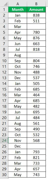
- In Excel, enter the following data containing both, the data cells and the empty cells.

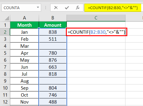
- Enter the following formula to count the data cells.
“=COUNTIF(range,”<>”&””)”
In the range argument, type B2:B30. Alternatively, select the range B2:B30 in the formula, as shown in the following image.

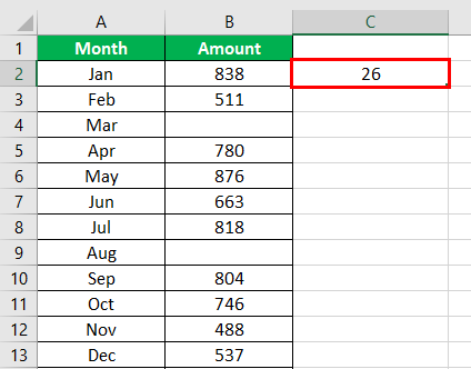
- Press the “Enter” key. The number of non-blank cells in the range B2:B30 appear in cell C2. The output is 26, as shown in the succeeding image.
This implies that there are 26 cells in the given range that contain a data value. This data can be a number, text, or any other value.

#2–Text Values
The steps to count non-empty cells within text values are listed as follows:
- Step 1: In Excel, enter the data as shown in the following image.
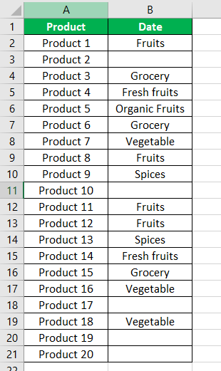
- Step 2: Select the range within which data needs to be checked for non-blank values. Enter the formula shown in the succeeding image.
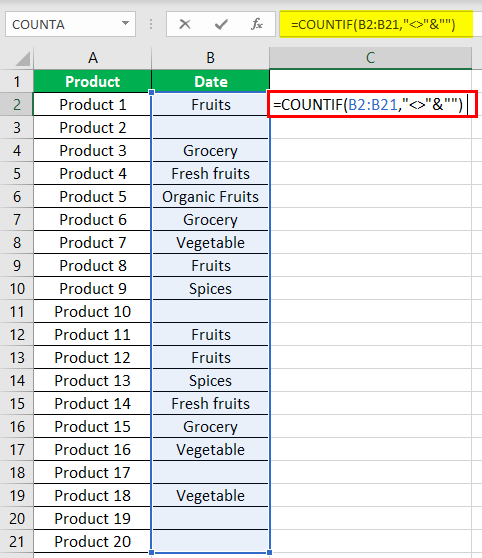
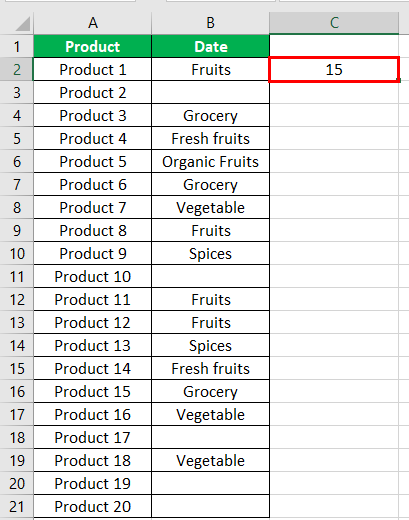
- Step 3: Press the “Enter” key. The number of non-blank cells in the range B2:B21 appear in cell C2. The output is 15, as shown in the succeeding image.
Hence, the COUNTIF not blank formula works with text values.
#3–Date Values
The steps to count non-empty cells, when the data consists of dates, are listed as follows:
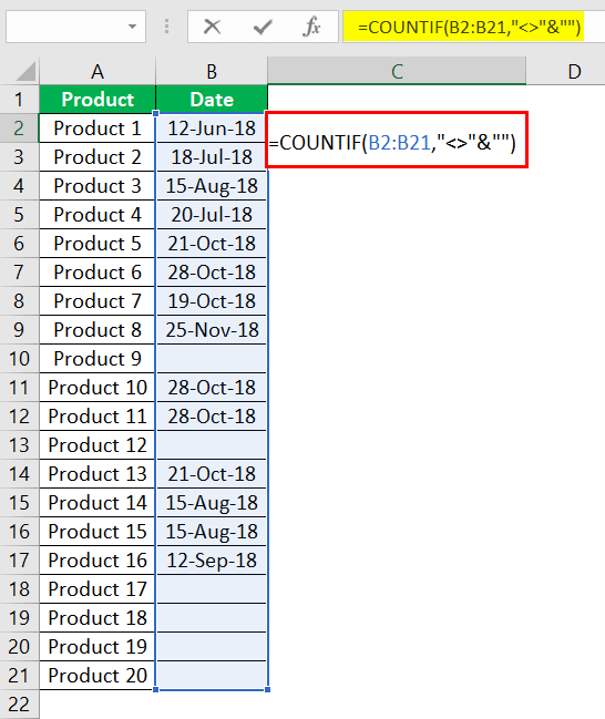
- Step 1: In Excel, enter the data as shown in the following image. Select the range whose data needs to be checked for non-blank values. Enter the following formula.
“=COUNTIF(B2:B21,”<>”&””)”
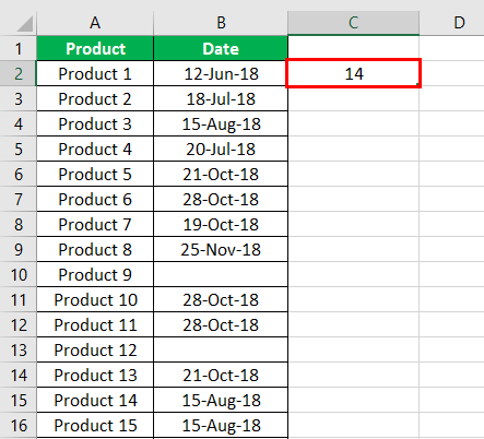
- Step 2: Press the “Enter” key. The number of non-blank cells in the range B2:B21 appear in cell C2. The output is 14, as shown in the succeeding image.
Hence, the COUNTIF not blank formula works with data that consists of date values.
The Characteristics of COUNTIF Not Blank Function
- It is case insensitive, implying that the output remains the same irrespective of whether the formula is entered in uppercase or lowercase.
- It works for data that consists of numbers, text, and date values.
- It works with greater than (>) and less than (<) operators.
- It is difficult to use the formula with long strings.
- The criteria (condition) must be specified within a pair of inverted commas to avoid errors.
Frequently Asked Questions
How is the COUNTIF formula used to count blanks?
The universal formula for counting blanks is stated as follows:
“COUNTIF(range,””)”
This formula works with all types of data values.
Note: Alternatively, the COUNTBLANK function can be used to count blank cells.
How does the COUNTIF function count the duplicate values?
The formula for counting the duplicate value is given as follows:
“COUNTIF(range,“duplicate value”)”
The “range” represents the range within which the duplicate values are to be counted. The “duplicate value” is the exact data value that is to be counted.
For example, to count the number of times the text “fruits” appears in the range A2:A10, we use “=COUNTIF(A2:A10,“fruits”).”
- The COUNTIF not blank function counts the non-blank cells within a given range.
- The generic formula of the COUNTIF not blank function is stated as–“COUNTIF (range,“<>”&””).”
- The criteria (condition) must be specified within a pair of inverted commas to avoid errors.
- The COUNTIF functionThe COUNTIF function in Excel counts the number of cells within a range based on pre-defined criteria. It is used to count cells that include dates, numbers, or text. For example, COUNTIF(A1:A10,”Trump”) will count the number of cells within the range A1:A10 that contain the text “Trump”
read more works for data that consists of numbers, text, and date values. - The COUNTIF formula gives the same output irrespective of whether the formula is entered in uppercase or lowercase.
Recommended Articles
This has been a guide to Excel COUNTIF not blank. Here we discuss how to use the COUNTIF function to count non-blank cells along with practical examples and a downloadable Excel template. You may learn more about Excel from the following articles –
- Not Equal in VBA
- COUNTIF with Multiple Criteria
- VLOOKUP Errors
- Use Not Equal to in Excel
- XML in Excel
The COUNTIF function counts cells in a range that meet a given condition, referred to as criteria. COUNTIF is a common, widely used function in Excel, and can be used to count cells that contain dates, numbers, and text. Note that COUNTIF can only apply a single condition. To count cells with multiple criteria, see the COUNTIFS function.
Syntax
The generic syntax for COUNTIF looks like this:
=COUNTIF(range,criteria)The COUNTIF function takes two arguments, range and criteria. Range is the range of cells to apply a condition to. Criteria is the condition to apply, along with any logical operators that are needed.
Applying criteria
The COUNTIF function supports logical operators (>,<,<>,<=,>=) and wildcards (*,?) for partial matching. The tricky part about using the COUNTIF function is the syntax used to apply criteria. COUNTIFS is in a group of eight functions that split logical criteria into two parts, range and criteria. Because of this design, each condition requires a separate range and criteria argument, and operators in the criteria must be enclosed in double quotes («»). The table below shows examples of the syntax needed for common criteria:
| Target | Criteria |
|---|---|
| Cells greater than 75 | «>75» |
| Cells equal to 100 | 100 or «100» |
| Cells less than or equal to 100 | «<=100» |
| Cells equal to «Red» | «red» |
| Cells not equal to «Red» | «<>red» |
| Cells that are blank «» | «» |
| Cells that are not blank | «<>» |
| Cells that begin with «X» | «x*» |
| Cells less than A1 | «<«&A1 |
| Cells less than today | «<«&TODAY() |
Notice the last two examples involve concatenation with the ampersand (&) character. Any time you are using a value from another cell, or using the result of a formula in criteria with a logical operator like «<«, you will need to concatenate. This is because Excel needs to evaluate cell references and formulas first to get a value, before that value can be joined to an operator.
Basic example
In the worksheet shown above, the following formulas are used in cells G5, G6, and G7:
=COUNTIF(D5:D12,">100") // count sales over 100
=COUNTIF(B5:B12,"jim") // count name = "jim"
=COUNTIF(C5:C12,"ca") // count state = "ca"
Notice COUNTIF is not case-sensitive, «CA» and «ca» are treated the same.
Double quotes («») in criteria
In general, text values need to be enclosed in double quotes («»), and numbers do not. However, when a logical operator is included with a number, the number and operator must be enclosed in quotes, as seen in the second example below:
=COUNTIF(A1:A10,100) // count cells equal to 100
=COUNTIF(A1:A10,">32") // count cells greater than 32
=COUNTIF(A1:A10,"jim") // count cells equal to "jim"
Value from another cell
A value from another cell can be included in criteria using concatenation. In the example below, COUNTIF will return the count of values in A1:A10 that are less than the value in cell B1. Notice the less than operator (which is text) is enclosed in quotes.
=COUNTIF(A1:A10,"<"&B1) // count cells less than B1
Not equal to
To construct «not equal to» criteria, use the «<>» operator surrounded by double quotes («»). For example, the formula below will count cells not equal to «red» in the range A1:A10:
=COUNTIF(A1:A10,"<>red") // not "red"
Blank cells
COUNTIF can count cells that are blank or not blank. The formulas below count blank and not blank cells in the range A1:A10:
=COUNTIF(A1:A10,"<>") // not blank
=COUNTIF(A1:A10,"") // blank
Note: be aware that COUNTIF treats formulas that return an empty string («») as not blank. See this example for some workarounds to this problem.
Dates
The easiest way to use COUNTIF with dates is to refer to a valid date in another cell with a cell reference. For example, to count cells in A1:A10 that contain a date greater than the date in B1, you can use a formula like this:
=COUNTIF(A1:A10, ">"&B1) // count dates greater than A1
Notice we must concatenate an operator to the date in B1. To use more advanced date criteria (i.e. all dates in a given month, or all dates between two dates) you’ll want to switch to the COUNTIFS function, which can handle multiple criteria.
The safest way to hardcode a date into COUNTIF is to use the DATE function. This ensures Excel will understand the date. To count cells in A1:A10 that contain a date less than April 1, 2020, you can use a formula like this
=COUNTIF(A1:A10,"<"&DATE(2020,4,1)) // dates less than 1-Apr-2020
Wildcards
The wildcard characters question mark (?), asterisk(*), or tilde (~) can be used in criteria. A question mark (?) matches any one character and an asterisk (*) matches zero or more characters of any kind. For example, to count cells in A1:A5 that contain the text «apple» anywhere, you can use a formula like this:
=COUNTIF(A1:A5,"*apple*") // cells that contain "apple"
To count cells in A1:A5 that contain any 3 text characters, you can use:
=COUNTIF(A1:A5,"???") // cells that contain any 3 characters
The tilde (~) is an escape character to match literal wildcards. For example, to count a literal question mark (?), asterisk(*), or tilde (~), add a tilde in front of the wildcard (i.e. ~?, ~*, ~~).
OR logic
The COUNTIF function is designed to apply just one condition. However, to count cells that contain «this OR that», you can use an array constant and the SUM function like this:
=SUM(COUNTIF(range,{"red","blue"})) // red or blue
The formula above will count cells in range that contain «red» or «blue». Essentially, COUNTIF returns two counts in an array (one for «red» and one for «blue») and the SUM function returns the sum. For more information, see this example.
Limitations
The COUNTIF function has some limitations you should be aware of:
- COUNTIF only supports a single condition. If you need to count cells using multiple criteria, use the COUNTIFS function.
- COUNTIF requires an actual range for the range argument; you can’t provide an array. This means you can’t alter values in range before applying criteria.
- COUNTIF is not case-sensitive. Use the EXACT function for case-sensitive counts.
- COUNTIFS has other quirks explained in this article.
The most common way to work around the limitations above is to use the SUMPRODUCT function. In the current version of Excel, another option is to use the newer BYROW and BYCOL functions.
Notes
- Text strings in criteria must be enclosed in double quotes («»), i.e. «apple», «>32», «app*»
- Cell references in criteria are not enclosed in quotes, i.e. «<«&A1
- The wildcard characters ? and * can be used in criteria. A question mark matches any one character and an asterisk matches any sequence of characters (zero or more).
- To match a literal question mark(?) or asterisk (*), use a tilde (~) like (~?, ~*).
- COUNTIF requires a range, you can’t substitute an array.
- COUNTIF returns incorrect results when used to match strings longer than 255 characters.
- COUNTIF will return a #VALUE error when referencing another workbook that is closed.
Author: Oscar Cronquist Article last updated on January 08, 2023
![]()
The COUNTIF function is very capable of counting non-empty values, I will show you how in this article. Excel can also highlight empty cells using Conditional formatting.
I will discuss and demonstrate the limitations of using the COUNTIF function and other equivalent functions that you also can use.
What’s on this page
- Count not blank cells — COUNTIF function
- Count not blank cells — COUNTA function
- COUNTIF and COUNTA function return unexpected results
- Count not blank cells — SUMPRODUCT function
- Get Excel *.xlsx file
1. Count not blank cells — COUNTIF function
![]()
Column B above has a few blank cells, they are in fact completely empty.
Formula in cell D3:
=COUNTIF(B3:B13,»<>»)
The first argument in the COUNTIF function is the cell range where you want to count matching cells to a specific value, the second argument is the value you want to count.
COUNTIF(range, criteria)
In this case, it is «<>» meaning not equal to and then nothing, so the COUNTIF function counts the number of cells that are not equal to nothing. In other words, cells that are not empty.

Back to top
2. Count not blank cells — COUNTA function
![]()
The COUNTA function is even easier to use, you don’t need to enter more than the cell range in one argument. The COUNTA function is designed to count non-empty cells.
COUNTA(value1, [value2], …)
Formula in cell D4:
=COUNTA(B3:B13)
Back to top
3. COUNTIF and COUNTA function return unexpected results
![]()
There are, however, situations where the COUNTIF and COUNTA function return unexpected results if you are not aware of how they work.
There are blank cells in column C, shown in the picture above, that look empty but they are not. Column D shows what they actually contain and column E shows the character length of the content.
Cell C5 and C9 contain a formula that returns a blank, both the COUNTIF and the COUNTA function count those cells as non-empty.
Cell C8 has two space characters and cell C12 has one space character, column E reveals their existence by counting character length. The COUNTIF and the COUNTA function count those cells as non-empty as well.
Back to top
4. Count not blank cells — SUMPRODUCT function
![]()
The following formula counts all non-empty values in cell range C3:C13 except formulas that return nothing. It checks if the values in cell range C3:C13 are not equal to nothing.
Formula in cell B16:
=SUMPRODUCT((C3:C13<>»»)*1)
Back to top
4.1 Explaining formula in cell B16
Step 1 — Check if cells are not empty
In this case, the logical expression counts cells that contain space characters but not formulas that return nothing.
The less than and the greater than characters are logical operators, the result are always boolean values.
C3:C13<>»»
returns
{TRUE; TRUE; FALSE; TRUE; TRUE; TRUE; FALSE; TRUE; TRUE; TRUE; TRUE}
Step 2 — Convert boolean values
The SUMPRODUCT function can’t sum boolean values, we need to multiply with one to create an array containing 0’s (zero) and 1’s.
They are their numerical equivalents:
True = 1
FALSE = 0 (zero)
(C3:C13<>»»)*1
becomes
{TRUE; TRUE; FALSE; TRUE; TRUE; TRUE; FALSE; TRUE; TRUE; TRUE; TRUE}*1
and returns
{1; 1; 0; 1; 1; 1; 0; 1; 1; 1; 1}
Step 3 — Sum numbers
Why use the SUMPRODUCT function and not the SUM function? The SUMPRODUCT function can perform calculations in the arguments without the need to enter the formula as an array formula.
Array formulas are great but if possible avoid as much as you can. Excel 365 users don’t have this problem, dynamic array formulas are entered as regular formulas.
SUMPRODUCT((C3:C13<>»»)*1)
becomes
SUMPRODUCT({1; 1; 0; 1; 1; 1; 0; 1; 1; 1; 1})
and returns 9 in cell B16.
Back to top
5. Regard formulas that return nothing to be blank and space characters to also be blank
![]()
The formula above in cell C16 counts only non-empty values, it considers formulas that return nothing to be blank and space characters to also be blank. This is made possible by the TRIM function that removes leading and ending space characters.
=SUMPRODUCT((TRIM(C3:C13)<>»»)*1)
Back to top
5.1 Explaining formula in cell B16
Step 1 — Remove space characters
TRIM(C3:C13)
returns
{«Green»; «Blue»; «»; «Red»; «Cyan»; «»; «»; «Yellow»; «Orange»; «»; «Brown»}
Step 2 — Identify not blank cells
TRIM(C3:C13)<>»»
becomes
{«Green»; «Blue»; «»; «Red»; «Cyan»; «»; «»; «Yellow»; «Orange»; «»; «Brown»}<>»»
and returns
{TRUE; TRUE; FALSE; TRUE; TRUE; FALSE; FALSE; TRUE; TRUE; FALSE; TRUE}
Step 3 — Multiply with 1
TRIM(C3:C13)<>»»)*1
becomes
{TRUE; TRUE; FALSE; TRUE; TRUE; FALSE; FALSE; TRUE; TRUE; FALSE; TRUE}*1
and returns
{1; 1; 0; 1; 1; 0; 0; 1; 1; 0; 1}
Step 4 — Sum numbers in array
SUMPRODUCT((TRIM(C3:C13)<>»»)*1)
becomes
SUMPRODUCT({1; 1; 0; 1; 1; 0; 0; 1; 1; 0; 1})
and returns 7.
Back to top
Latest updated articles.
More than 300 Excel functions with detailed information including syntax, arguments, return values, and examples for most of the functions used in Excel formulas.
More than 1300 formulas organized in subcategories.
Excel Tables simplifies your work with data, adding or removing data, filtering, totals, sorting, enhance readability using cell formatting, cell references, formulas, and more.
Allows you to filter data based on selected value , a given text, or other criteria. It also lets you filter existing data or move filtered values to a new location.
Lets you control what a user can type into a cell. It allows you to specifiy conditions and show a custom message if entered data is not valid.
Lets the user work more efficiently by showing a list that the user can select a value from. This lets you control what is shown in the list and is faster than typing into a cell.
Lets you name one or more cells, this makes it easier to find cells using the Name box, read and understand formulas containing names instead of cell references.
The Excel Solver is a free add-in that uses objective cells, constraints based on formulas on a worksheet to perform what-if analysis and other decision problems like permutations and combinations.
An Excel feature that lets you visualize data in a graph.
Format cells or cell values based a condition or criteria, there a multiple built-in Conditional Formatting tools you can use or use a custom-made conditional formatting formula.
Lets you quickly summarize vast amounts of data in a very user-friendly way. This powerful Excel feature lets you then analyze, organize and categorize important data efficiently.
VBA stands for Visual Basic for Applications and is a computer programming language developed by Microsoft, it allows you to automate time-consuming tasks and create custom functions.
A program or subroutine built in VBA that anyone can create. Use the macro-recorder to quickly create your own VBA macros.
UDF stands for User Defined Functions and is custom built functions anyone can create.
A list of all published articles.
Excel has many functions where a user needs to specify a single or multiple criteria to get the result. For example, if you want to count cells based on multiple criteria, you can use the COUNTIF or COUNTIFS functions in Excel.
This tutorial covers various ways of using a single or multiple criteria in COUNTIF and COUNTIFS function in Excel.
While I will primarily be focussing on COUNTIF and COUNTIFS functions in this tutorial, all these examples can also be used in other Excel functions that take multiple criteria as inputs (such as SUMIF, SUMIFS, AVERAGEIF, and AVERAGEIFS).
An Introduction to Excel COUNTIF and COUNTIFS Functions
Let’s first get a grip on using COUNTIF and COUNTIFS functions in Excel.
Excel COUNTIF Function (takes Single Criteria)
Excel COUNTIF function is best suited for situations when you want to count cells based on a single criterion. If you want to count based on multiple criteria, use COUNTIFS function.
Syntax
=COUNTIF(range, criteria)
Input Arguments
- range – the range of cells which you want to count.
- criteria – the criteria that must be evaluated against the range of cells for a cell to be counted.
Excel COUNTIFS Function (takes Multiple Criteria)
Excel COUNTIFS function is best suited for situations when you want to count cells based on multiple criteria.
Syntax
=COUNTIFS(criteria_range1, criteria1, [criteria_range2, criteria2]…)
Input Arguments
- criteria_range1 – The range of cells for which you want to evaluate against criteria1.
- criteria1 – the criteria which you want to evaluate for criteria_range1 to determine which cells to count.
- [criteria_range2] – The range of cells for which you want to evaluate against criteria2.
- [criteria2] – the criteria which you want to evaluate for criteria_range2 to determine which cells to count.
Now let’s have a look at some examples of using multiple criteria in COUNTIF functions in Excel.
Using NUMBER Criteria in Excel COUNTIF Functions
#1 Count Cells when Criteria is EQUAL to a Value
To get the count of cells where the criteria argument is equal to a specified value, you can either directly enter the criteria or use the cell reference that contains the criteria.
Below is an example where we count the cells that contain the number 9 (which means that the criteria argument is equal to 9). Here is the formula:
=COUNTIF($B$2:$B$11,D3)

In the above example (in the pic), the criteria is in cell D3. You can also enter the criteria directly into the formula. For example, you can also use:
=COUNTIF($B$2:$B$11,9)
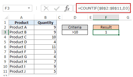
#2 Count Cells when Criteria is GREATER THAN a Value
To get the count of cells with a value greater than a specified value, we use the greater than operator (“>”). We could either use it directly in the formula or use a cell reference that has the criteria.
Whenever we use an operator in criteria in Excel, we need to put it within double quotes. For example, if the criteria is greater than 10, then we need to enter “>10” as the criteria (see pic below):
Here is the formula:
=COUNTIF($B$2:$B$11,”>10″)

You can also have the criteria in a cell and use the cell reference as the criteria. In this case, you need NOT put the criteria in double quotes:
=COUNTIF($B$2:$B$11,D3)
There could also be a case when you want the criteria to be in a cell, but don’t want it with the operator. For example, you may want the cell D3 to have the number 10 and not >10.
In that case, you need to create a criteria argument which is a combination of operator and cell reference (see pic below):
=COUNTIF($B$2:$B$11,”>”&D3)
 NOTE: When you combine an operator and a cell reference, the operator is always in double quotes. The operator and cell reference are joined by an ampersand (&).
#3 Count Cells when Criteria is LESS THAN a Value
To get the count of cells with a value less than a specified value, we use the less than operator (“<“). We could either use it directly in the formula or use a cell reference that has the criteria.
Whenever we use an operator in criteria in Excel, we need to put it within double quotes. For example, if the criterion is that the number should be less than 5, then we need to enter “<5” as the criteria (see pic below):
=COUNTIF($B$2:$B$11,”<5″)

You can also have the criteria in a cell and use the cell reference as the criteria. In this case, you need NOT put the criteria in double quotes (see pic below):
=COUNTIF($B$2:$B$11,D3)

Also, there could be a case when you want the criteria to be in a cell, but don’t want it with the operator. For example, you may want the cell D3 to have the number 5 and not <5.
In that case, you need to create a criteria argument which is a combination of operator and cell reference:
=COUNTIF($B$2:$B$11,”<“&D3)

NOTE: When you combine an operator and a cell reference, the operator is always in double quotes. The operator and cell reference are joined by an ampersand (&).
#4 Count Cells with Multiple Criteria – Between Two Values
To get a count of values between two values, we need to use multiple criteria in the COUNTIF function.
Here are two methods of doing this:
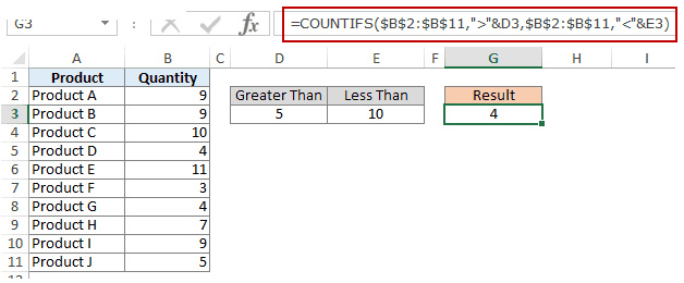
METHOD 1: Using COUNTIFS function
COUNTIFS function can handle multiple criteria as arguments and counts the cells only when all the criteria are TRUE. To count cells with values between two specified values (say 5 and 10), we can use the following COUNTIFS function:
=COUNTIFS($B$2:$B$11,”>5″,$B$2:$B$11,”<10″)

NOTE: The above formula does not count cells that contain 5 or 10. If you want to include these cells, use greater than equal to (>=) and less than equal to (<=) operators. Here is the formula:
=COUNTIFS($B$2:$B$11,”>=5″,$B$2:$B$11,”<=10″)
You can also have these criteria in cells and use the cell reference as the criteria. In this case, you need NOT put the criteria in double quotes (see pic below):

You can also use a combination of cells references and operators (where the operator is entered directly in the formula). When you combine an operator and a cell reference, the operator is always in double quotes. The operator and cell reference are joined by an ampersand (&).
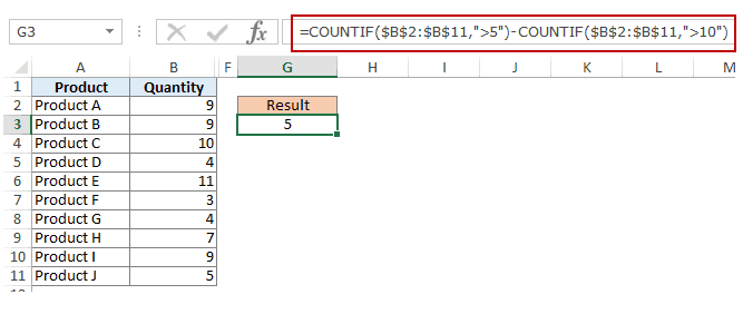
METHOD 2: Using two COUNTIF functions
If you have multiple criteria, you can either use COUNTIFS or create a combination of COUNTIF functions. The formula below would also do the same thing:
=COUNTIF($B$2:$B$11,”>5″)-COUNTIF($B$2:$B$11,”>10″)
In the above formula, we first find the number of cells that have a value greater than 5 and we subtract the count of cells with a value greater than 10. This would give us the result as 5 (which is the number of cells that have values more than 5 and less than equal to 10).
If you want the formula to include both 5 and 10, use the following formula instead:
=COUNTIF($B$2:$B$11,”>=5″)-COUNTIF($B$2:$B$11,”>10″)
If you want the formula to exclude both ‘5’ and ’10’ from the counting, use the following formula:
=COUNTIF($B$2:$B$11,”>=5″)-COUNTIF($B$2:$B$11,”>10″)-COUNTIF($B$2:$B$11,10)
You can have these criteria in cells and use the cells references, or you can use a combination of operators and cells references.
Using TEXT Criteria in Excel Functions
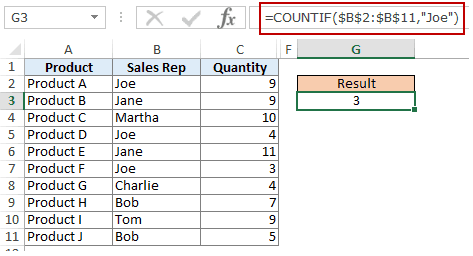
#1 Count Cells when Criteria is EQUAL to a Specified text
To count cells that contain an exact match of the specified text, we can simply use that text as the criteria. For example, in the dataset (shown below in the pic), if I want to count all the cells with the name Joe in it, I can use the below formula:
=COUNTIF($B$2:$B$11,”Joe”)
Since this is a text string, I need to put the text criteria in double quotes.
You can also have the criteria in a cell and then use that cell reference (as shown below):
=COUNTIF($B$2:$B$11,E3)

NOTE: You can get wrong results if there are leading/trailing spaces in the criteria or criteria range. Make sure you clean the data before using these formulas.
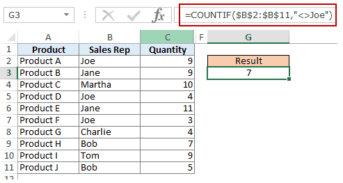
#2 Count Cells when Criteria is NOT EQUAL to a Specified text
Similar to what we saw in the above example, you can also count cells that do not contain a specified text. To do this, we need to use the not equal to operator (<>).
Suppose you want to count all the cells that do not contain the name JOE, here is the formula that will do it:
=COUNTIF($B$2:$B$11,”<>Joe”)
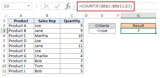
You can also have the criteria in a cell and use the cell reference as the criteria. In this case, you need NOT put the criteria in double quotes (see pic below):
=COUNTIF($B$2:$B$11,E3)
There could also be a case when you want the criteria to be in a cell but don’t want it with the operator. For example, you may want the cell D3 to have the name Joe and not <>Joe.
In that case, you need to create a criteria argument which is a combination of operator and cell reference (see pic below):
=COUNTIF($B$2:$B$11,”<>”&E3)
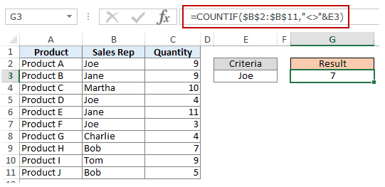
When you combine an operator and a cell reference, the operator is always in double quotes. The operator and cell reference are joined by an ampersand (&).
Using DATE Criteria in Excel COUNTIF and COUNTIFS Functions
Excel store date and time as numbers. So we can use it the same way we use numbers.
#1 Count Cells when Criteria is EQUAL to a Specified Date
To get the count of cells that contain the specified date, we would use the equal to operator (=) along with the date.
To use the date, I recommend using the DATE function, as it gets rid of any possibility of error in the date value. So, for example, if I want to use the date September 1, 2015, I can use the DATE function as shown below:
=DATE(2015,9,1)
This formula would return the same date despite regional differences. For example, 01-09-2015 would be September 1, 2015 according to the US date syntax and January 09, 2015 according to the UK date syntax. However, this formula would always return September 1, 2105.
Here is the formula to count the number of cells that contain the date 02-09-2015:
=COUNTIF($A$2:$A$11,DATE(2015,9,2))

#2 Count Cells when Criteria is BEFORE or AFTER to a Specified Date
To count cells that contain date before or after a specified date, we can use the less than/greater than operators.
For example, if I want to count all the cells that contain a date that is after September 02, 2015, I can use the formula:
=COUNTIF($A$2:$A$11,”>”&DATE(2015,9,2))

Similarly, you can also count the number of cells before a specified date. If you want to include a date in the counting, use and ‘equal to’ operator along with ‘greater than/less than’ operator.
You can also use a cell reference that contains a date. In this case, you need to combine the operator (within double quotes) with the date using an ampersand (&).
See example below:
=COUNTIF($A$2:$A$11,”>”&F3)

#3 Count Cells with Multiple Criteria – Between Two Dates
To get a count of values between two values, we need to use multiple criteria in the COUNTIF function.
We can do this using two methods – One single COUNTIFS function or two COUNTIF functions.
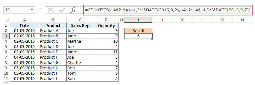
METHOD 1: Using COUNTIFS function
COUNTIFS function can take multiple criteria as the arguments and counts the cells only when all the criteria are TRUE. To count cells with values between two specified dates (say September 2 and September 7), we can use the following COUNTIFS function:
=COUNTIFS($A$2:$A$11,”>”&DATE(2015,9,2),$A$2:$A$11,”<“&DATE(2015,9,7))
The above formula does not count cells that contain the specified dates. If you want to include these dates as well, use greater than equal to (>=) and less than equal to (<=) operators. Here is the formula:
=COUNTIFS($A$2:$A$11,”>=”&DATE(2015,9,2),$A$2:$A$11,”<=”&DATE(2015,9,7))
You can also have the dates in a cell and use the cell reference as the criteria. In this case, you can not have the operator with the date in the cells. You need to manually add operators in the formula (in double quotes) and add cell reference using an ampersand (&). See the pic below:
=COUNTIFS($A$2:$A$11,”>”&F3,$A$2:$A$11,”<“&G3)

METHOD 2: Using COUNTIF functions
If you have multiple criteria, you can either use one COUNTIFS function or create a combination of two COUNTIF functions. The formula below would also do the trick:
=COUNTIF($A$2:$A$11,”>”&DATE(2015,9,2))-COUNTIF($A$2:$A$11,”>”&DATE(2015,9,7))
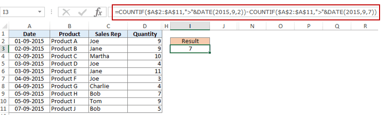
In the above formula, we first find the number of cells that have a date after September 2 and we subtract the count of cells with dates after September 7. This would give us the result as 7 (which is the number of cells that have dates after September 2 and on or before September 7).
If you don’t want the formula to count both September 2 and September 7, use the following formula instead:
=COUNTIF($A$2:$A$11,”>=”&DATE(2015,9,2))-COUNTIF($A$2:$A$11,”>”&DATE(2015,9,7))

If you want to exclude both the dates from counting, use the following formula:
=COUNTIF($A$2:$A$11,”>”&DATE(2015,9,2))-COUNTIF($A$2:$A$11,”>”&DATE(2015,9,7)-COUNTIF($A$2:$A$11,DATE(2015,9,7)))
Also, you can have the criteria dates in cells and use the cells references (along with operators in double quotes joined using ampersand).
Using WILDCARD CHARACTERS in Criteria in COUNTIF & COUNTIFS Functions
There are three wildcard characters in Excel:
- * (asterisk) – It represents any number of characters. For example, ex* could mean excel, excels, example, expert, etc.
- ? (question mark) – It represents one single character. For example, Tr?mp could mean Trump or Tramp.
- ~ (tilde) – It is used to identify a wildcard character (~, *, ?) in the text.
You can use COUNTIF function with wildcard characters to count cells when other inbuilt count function fails. For example, suppose you have a data set as shown below:
Now let’s take various examples:
#1 Count Cells that contain Text
To count cells with text in it, we can use the wildcard character * (asterisk). Since asterisk represents any number of characters, it would count all cells that have any text in it. Here is the formula:
=COUNTIFS($C$2:$C$11,”*”)
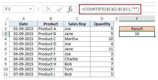
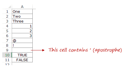
Note: The formula above ignores cells that contain numbers, blank cells, and logical values, but would count the cells contain an apostrophe (and hence appear blank) or cells that contain empty string (=””) which may have been returned as a part of a formula.
Here is a detailed tutorial on handling cases where there is an empty string or apostrophe.
Here is a detailed tutorial on handling cases where there are empty strings or apostrophes.
Below is a video that explains different scenarios of counting cells with text in it.
#2 Count Non-blank Cells
If you are thinking of using COUNTA function, think again.
Try it and it might fail you. COUNTA will also count a cell that contains an empty string (often returned by formulas as =”” or when people enter only an apostrophe in a cell). Cells that contain empty strings look blank but are not, and thus counted by the COUNTA function.
COUNTA will also count a cell that contains an empty string (often returned by formulas as =”” or when people enter only an apostrophe in a cell). Cells that contain empty strings look blank but are not, and thus counted by the COUNTA function.
So if you use the formula =COUNTA(A1:A11), it returns 11, while it should return 10.
Here is the fix:
=COUNTIF($A$1:$A$11,”?*”)+COUNT($A$1:$A$11)+SUMPRODUCT(–ISLOGICAL($A$1:$A$11))
Let’s understand this formula by breaking it down:
#3 Count Cells that contain specific text
Let’s say we want to count all the cells where the sales rep name begins with J. This can easily be achieved by using a wildcard character in COUNTIF function. Here is the formula:
=COUNTIFS($C$2:$C$11,”J*”)

The criteria J* specifies that the text in a cell should begin with J and can contain any number of characters.
If you want to count cells that contain the alphabet anywhere in the text, flank it with an asterisk on both sides. For example, if you want to count cells that contain the alphabet “a” in it, use *a* as the criteria.
This article is unusually long compared to my other articles. Hope you have enjoyed it. Let me know your thoughts by leaving a comment.
You May Also Find the following Excel tutorials useful:
- Count the number of words in Excel.
- Count Cells Based on Background Color in Excel.
- How to Sum a Column in Excel (5 Really Easy Ways)