
Содержание
- SUMIF function
- Syntax
- IF function – nested formulas and avoiding pitfalls
- Remarks
- Examples
- Additional examples
- Did you know?
- Need more help?
- SUMIF and COUNTIF in Excel
- Criteria are Text Values
- Example: Sum of Sales where Category equals «student»
- Not Equal To (<>)
- Example: Sum of Sales where Model is NOT equal to «B»
- Example: Sum of Sales where Category does NOT contain the letter «u»
- Criteria is an Alphabetical Text Comparison
- Example: Sum of Sales where Model is less than «C»
- Criteria is a Numeric Comparison
- Example: Number of products priced over $40
- Criteria matches Blank Cells or Empty Cells
- Example: Count of products where On Sale is blank
- Criteria matches Non-Blank Cells
- Example: Number of products on sale (where On Sale is not blank)
- Criteria includes a Cell Reference
- Example: Sum of Sales where Price is greater than the value in cell H3
- Criteria is In Another Cell
- Example: Sum of Sales using the criteria defined in cell K9
- Multiple Criteria
- Example: Sum of Sales where Category = «student» AND Price > 30
- Example: SUMIFS between two dates
- 2) Using Dates as Criteria
- Comparison to TODAY
- 3) SUMIFS Example: Income and Expense Report
- 4) SUMIF and COUNTIF Between Two Numbers (1 1 AND x 1″,range,» 3 are usually easier to handle by evaluating each condition separately and then adding the results. The two formulas below do essentially the same thing.
- Use SUMPRODUCT for overlapping OR conditions
- Sum of Sales where Model is equal to A or B.
- Sum of Sales where Model = «A» or Price > 45
- 6) Case-Sensitive SUMIF and COUNTIF
- Sum of Sales where Category exactly matches «student» (case-sensitive)
- Sum of Sales where Category contains «Stu» (case-sensitive)
- 7) MAXIF or MINIF Formula
- Example: Find the maximum Price where Model = «A»
-
 Summary of Different Criteria Types
 - 9) Other Notes
- Comments
 Summary of Different Criteria Types
SUMIF function
You use the SUMIF function to sum the values in a range that meet criteria that you specify. For example, suppose that in a column that contains numbers, you want to sum only the values that are larger than 5. You can use the following formula: =SUMIF(B2:B25,»>5″)

This video is part of a training course called Add numbers in Excel.
If you want, you can apply the criteria to one range and sum the corresponding values in a different range. For example, the formula =SUMIF(B2:B5, «John», C2:C5) sums only the values in the range C2:C5, where the corresponding cells in the range B2:B5 equal «John.»
To sum cells based on multiple criteria, see SUMIFS function.
Important: The SUMIF function returns incorrect results when you use it to match strings longer than 255 characters or to the string #VALUE!.
Syntax
SUMIF(range, criteria, [sum_range])
The SUMIF function syntax has the following arguments:
range Required. The range of cells that you want evaluated by criteria. Cells in each range must be numbers or names, arrays, or references that contain numbers. Blank and text values are ignored. The selected range may contain dates in standard Excel format (examples below).
criteria Required. The criteria in the form of a number, expression, a cell reference, text, or a function that defines which cells will be added. Wildcard characters can be included — a question mark (?) to match any single character, an asterisk (*) to match any sequence of characters. If you want to find an actual question mark or asterisk, type a tilde (
) preceding the character.
For example, criteria can be expressed as 32, «>32», B5, «3?», «apple*», «*
Important: Any text criteria or any criteria that includes logical or mathematical symbols must be enclosed in double quotation marks ( «). If the criteria is numeric, double quotation marks are not required.
sum_range Optional. The actual cells to add, if you want to add cells other than those specified in the range argument. If the sum_range argument is omitted, Excel adds the cells that are specified in the range argument (the same cells to which the criteria is applied).
Sum_range should be the same size and shape as range. If it isn’t, performance may suffer, and the formula will sum a range of cells that starts with the first cell in sum_range but has the same dimensions as range. For example:
Источник
IF function – nested formulas and avoiding pitfalls
The IF function allows you to make a logical comparison between a value and what you expect by testing for a condition and returning a result if True or False.
=IF(Something is True, then do something, otherwise do something else)
So an IF statement can have two results. The first result is if your comparison is True, the second if your comparison is False.
IF statements are incredibly robust, and form the basis of many spreadsheet models, but they are also the root cause of many spreadsheet issues. Ideally, an IF statement should apply to minimal conditions, such as Male/Female, Yes/No/Maybe, to name a few, but sometimes you might need to evaluate more complex scenarios that require nesting* more than 3 IF functions together.
* “Nesting” refers to the practice of joining multiple functions together in one formula.
Use the IF function, one of the logical functions, to return one value if a condition is true and another value if it’s false.
IF(logical_test, value_if_true, [value_if_false])
The condition you want to test.
The value that you want returned if the result of logical_test is TRUE.
The value that you want returned if the result of logical_test is FALSE.
While Excel will allow you to nest up to 64 different IF functions, it’s not at all advisable to do so. Why?
Multiple IF statements require a great deal of thought to build correctly and make sure that their logic can calculate correctly through each condition all the way to the end. If you don’t nest your formula 100% accurately, then it might work 75% of the time, but return unexpected results 25% of the time. Unfortunately, the odds of you catching the 25% are slim.
Multiple IF statements can become incredibly difficult to maintain, especially when you come back some time later and try to figure out what you, or worse someone else, was trying to do.
If you find yourself with an IF statement that just seems to keep growing with no end in sight, it’s time to put down the mouse and rethink your strategy.
Let’s look at how to properly create a complex nested IF statement using multiple IFs, and when to recognize that it’s time to use another tool in your Excel arsenal.
Examples
Following is an example of a relatively standard nested IF statement to convert student test scores to their letter grade equivalent.
 97,»A+»,IF(B2>93,»A»,IF(B2>89,»A-«,IF(B2>87,»B+»,IF(B2>83,»B»,IF(B2>79,»B-«,IF(B2>77,»C+»,IF(B2>73,»C»,IF(B2>69,»C-«,IF(B2>57,»D+»,IF(B2>53,»D»,IF(B2>49,»D-«,»F»))))))))))))» loading=»lazy»>
This complex nested IF statement follows a straightforward logic:
If the Test Score (in cell D2) is greater than 89, then the student gets an A
If the Test Score is greater than 79, then the student gets a B
If the Test Score is greater than 69, then the student gets a C
If the Test Score is greater than 59, then the student gets a D
Otherwise the student gets an F
This particular example is relatively safe because it’s not likely that the correlation between test scores and letter grades will change, so it won’t require much maintenance. But here’s a thought – what if you need to segment the grades between A+, A and A- (and so on)? Now your four condition IF statement needs to be rewritten to have 12 conditions! Here’s what your formula would look like now:
It’s still functionally accurate and will work as expected, but it takes a long time to write and longer to test to make sure it does what you want. Another glaring issue is that you’ve had to enter the scores and equivalent letter grades by hand. What are the odds that you’ll accidentally have a typo? Now imagine trying to do this 64 times with more complex conditions! Sure, it’s possible, but do you really want to subject yourself to this kind of effort and probable errors that will be really hard to spot?
Tip: Every function in Excel requires an opening and closing parenthesis (). Excel will try to help you figure out what goes where by coloring different parts of your formula when you’re editing it. For instance, if you were to edit the above formula, as you move the cursor past each of the ending parentheses “)”, its corresponding opening parenthesis will turn the same color. This can be especially useful in complex nested formulas when you’re trying to figure out if you have enough matching parentheses.
Additional examples
Following is a very common example of calculating Sales Commission based on levels of Revenue achievement.
 15000,20%,IF(C9>12500,17.5%,IF(C9>10000,15%,IF(C9>7500,12.5%,IF(C9>5000,10%,0)))))» loading=»lazy»>
This formula says IF(C9 is Greater Than 15,000 then return 20%, IF(C9 is Greater Than 12,500 then return 17.5%, and so on.
While it’s remarkably similar to the earlier Grades example, this formula is a great example of how difficult it can be to maintain large IF statements – what would you need to do if your organization decided to add new compensation levels and possibly even change the existing dollar or percentage values? You’d have a lot of work on your hands!
Tip: You can insert line breaks in the formula bar to make long formulas easier to read. Just press ALT+ENTER before the text you want to wrap to a new line.
Here is an example of the commission scenario with the logic out of order:
 5000,10%,IF(C9>7500,12.5%,IF(C9>10000,15%,IF(C9>12500,17.5%,IF(C9>15000,20%,0)))))» loading=»lazy»>
Can you see what’s wrong? Compare the order of the Revenue comparisons to the previous example. Which way is this one going? That’s right, it’s going from bottom up ($5,000 to $15,000), not the other way around. But why should that be such a big deal? It’s a big deal because the formula can’t pass the first evaluation for any value over $5,000. Let’s say you’ve got $12,500 in revenue – the IF statement will return 10% because it is greater than $5,000, and it will stop there. This can be incredibly problematic because in a lot of situations these types of errors go unnoticed until they’ve had a negative impact. So knowing that there are some serious pitfalls with complex nested IF statements, what can you do? In most cases, you can use the VLOOKUP function instead of building a complex formula with the IF function. Using VLOOKUP, you first need to create a reference table:

This formula says to look for the value in C2 in the range C5:C17. If the value is found, then return the corresponding value from the same row in column D.

Similarly, this formula looks for the value in cell B9 in the range B2:B22. If the value is found, then return the corresponding value from the same row in column C.
Note: Both of these VLOOKUPs use the TRUE argument at the end of the formulas, meaning we want them to look for an approxiate match. In other words, it will match the exact values in the lookup table, as well as any values that fall between them. In this case the lookup tables need to be sorted in Ascending order, from smallest to largest.
VLOOKUP is covered in much more detail here, but this is sure a lot simpler than a 12-level, complex nested IF statement! There are other less obvious benefits as well:
VLOOKUP reference tables are right out in the open and easy to see.
Table values can be easily updated and you never have to touch the formula if your conditions change.
If you don’t want people to see or interfere with your reference table, just put it on another worksheet.
Did you know?
There is now an IFS function that can replace multiple, nested IF statements with a single function. So instead of our initial grades example, which has 4 nested IF functions:
It can be made much simpler with a single IFS function:
The IFS function is great because you don’t need to worry about all of those IF statements and parentheses.
Note: This feature is only available if you have a Microsoft 365 subscription. If you are a Microsoft 365subscriber, make sure you have the latest version of Office.
Need more help?
You can always ask an expert in the Excel Tech Community or get support in the Answers community.
Источник
SUMIF and COUNTIF in Excel
SUMIF, SUMIFS, COUNTIF, and COUNTIFS are extremely useful and powerful for data analysis. If there was an Excel Function Hall of Fame, this family of functions ought to be included. In this article, I’ll demonstrate a bunch of different ways to use these functions, focusing mainly on all the different criteria types.

The SUMIF and COUNTIF functions allow you to conditionally sum or count cells based on a single condition, and are compatible with almost all versions of Excel:
The SUMIFS and COUNTIFS functions allow you to use multiple criteria, but are only available beginning with Excel 2007:
AVERAGEIF and AVERAGEIFS are also part of this family of functions and have the same syntax as SUMIF and SUMIFS.
This Article (bookmarks):
Criteria are Text Values
Example: Sum of Sales where Category equals «student»
NOTE This formula will also match «Student» because the SUMIF family of functions are not case-sensitive. You can use wildcard characters within the text string, such as «?s*» to match values where the second letter is s.
Not Equal To (<>)
Example: Sum of Sales where Model is NOT equal to «B»
Example: Sum of Sales where Category does NOT contain the letter «u»
Criteria is an Alphabetical Text Comparison
Example: Sum of Sales where Model is less than «C»
Criteria is a Numeric Comparison
Example: Number of products priced over $40
NOTE When using numeric criteria, COUNTIF and SUMIF ignore text values. Numeric date values can be an exception to that (see below for date comparisons).
Criteria matches Blank Cells or Empty Cells
Example: Count of products where On Sale is blank
Criteria matches Non-Blank Cells
Example: Number of products on sale (where On Sale is not blank)
Criteria includes a Cell Reference
Example: Sum of Sales where Price is greater than the value in cell H3
Criteria is In Another Cell
Example: Sum of Sales using the criteria defined in cell K9
NOTE This technique is useful when you want to allow the user to choose or enter different criteria or search strings.
The cell K9 could contain a value like «student» or «40» or a criteria string such as «>40» or «<>student»
Multiple Criteria
Example: Sum of Sales where Category = «student» AND Price > 30
Example: SUMIFS between two dates
NOTE The SUMIFS, COUNTIFS, and AVERAGEIFS functions are used for multiple AND conditions. Formulas for OR conditions are a bit more tricky (see below).
2) Using Dates as Criteria
When using dates as criteria for the COUNTIF and SUMIF functions, Excel does some interesting things, depending on whether you are using «=» or » , =, Excel still recognizes the criteria as a date, but it does not convert text values in the criteria_range to date values.
Comparison to TODAY
You can use the TODAY function to make comparisons based on the current date, like this:
3) SUMIFS Example: Income and Expense Report
SUMIFS is very useful in account registers, budgeting, and money management spreadsheets for summarizing expenses by category and between two dates.
The SUMIFS example below sums the Amount column with 3 criteria: (1) the Category matches «Fuel», (2) the Date is greater than or equal to the start date, and (3) the Date is less than or equal to the end date.
The following screenshot shows an example from the download file:

4) SUMIF and COUNTIF Between Two Numbers (1 1 AND x 1″,range,» 3 are usually easier to handle by evaluating each condition separately and then adding the results. The two formulas below do essentially the same thing.
| Condition | Formula |
|---|---|
| x 3″) | |
| x 3″>)) |
To avoid double-counting cells, the conditions must not overlap. For example, the condition «=*e*» would overlap with the condition «=yes». The condition » 20″. If the conditions overlap, you may end up counting or adding a value twice. If there is a possibility of conditions overlapping, then you may need to use a SUMPRODUCT formula as explained below.
Use SUMPRODUCT for overlapping OR conditions
The key to avoid double-counting is to recognize that FALSE+FALSE=0 and TRUE+FALSE=1 and TRUE+TRUE=2. This means that for a logical OR condition to be true, we can check whether the sum of two or more conditions is > 0.
Sum of Sales where Model is equal to A or B.
Sum of Sales where Model = «A» or Price > 45
6) Case-Sensitive SUMIF and COUNTIF
The SUMIF family does not have a case-sensitive option, so we need to resort back to using array formulas or SUMPRODUCT. The FIND and EXACT functions both provide a way to do case-sensitive matches.
Sum of Sales where Category exactly matches «student» (case-sensitive)
Sum of Sales where Category contains «Stu» (case-sensitive)
7) MAXIF or MINIF Formula
MAXIFS and MINIFS are new Excel functions available in the latest releases (Excel for Microsoft 365, Excel 2019). Their syntax is similar to SUMIFS, allowing you to use multiple criteria.
Older versions of Excel do not have the MAXIFS or MINIFS functions, but you can use an array formula like this (remember to press Ctrl+Shift+Enter):
Example: Find the maximum Price where Model = «A»
Summary of Different Criteria Types
| CRITERIA TYPE | EXAMPLE | MATCHES . |
|---|---|---|
| Text Value | «yes» or «=yes» | «yes» or «Yes» (not case-sensitive), the equal sign is optional |
| Text Value with Wildcards | «=?s*» | text values where the second letter is «s» or «S» |
| Alphabetical Text Comparison | » =20″ | numeric values greater than or equal to 20 |
| Not Equal to | «<>0″ | values not equal to the value 0 |
| Non-Blank | «<>« | values that are not blank (formulas returning «» are not blank) |
| Blank or Empty | «» | values that are blank and formulas that return «» |
| Equal to a Cell Value | A42 or «=»&A42 | values equal to the value in cell A42 |
| Comparison to a Cell Value | «>»&A42 | values greater than the value in cell A42 |
| Equal to a Date | «=3/1/17» | date values equal to 3/1/17 as well as text values such as «3/1/17» or «Mar 1, 2017» |
| a Date | «>1/1/2017» | date values greater than 1/1/2017 (text values are ignored) |
Some criteria, such as case-sensitive matches, may only be possible with array formulas or SUMPRODUCT.
You don’t use the functions AND, NOT, OR, ISBLANK, ISNUMBER, ISERROR, or other similar functions as criteria for SUMIF and COUNTIF. However, you can use these functions within a SUMPRODUCT formula (but that isn’t within the scope of this article).
9) Other Notes
- Comparisons are based on the value stored in the cell, not on how the cell is formatted.
- Error values in both the sum_range and criteria_range are ignored.
- SUMIFS and COUNTIFS formulas are generally faster than their SUMPRODUCT or array formula counterparts.
- The sum_range and criteria_range arguments can be references (e.g. A2:A42), named ranges or formulas that return a range (such as INDEX, OFFSET, or INDIRECT).
- Normally, you’ll want the sum_range and criteria_range to be the same length. See the documentation on the Microsoft sites (referenced below) for information about what happens when the sum_range and criteria_range are not the same length.
- The COUNTIF and SUMIF criteria can be a range (e.g. A2:A3) if you enter the formula as an array formula using Ctrl+Shift+Enter.
- The COUNTIF and SUMIF criteria can be a list such as <«>1″,»
Kindly assist me to count ‘AA’, ‘AB’,’AC and ‘AD’ from ‘X’, ‘Y’ and ‘Z’.
Total AA, AB, AC and AD is 2500 from X, Y and Z
@Saad, I’m afraid I don’t know what you mean. Are you referring to AA, AB, X, Y, etc as column labels? If you can be more specific, that would help.
Row A Row B
07:00:00 1
07:02:00 2
Result 07:00:00 3
How to calculate
@Manju … You would need to provide more information. Please ask general questions like this via an Excel forum.
I’m looking at the Money Management Template 2.1 and I see you made extensive use of the offset command in the sum command and was wonder why. For example in the balance column, SUM(M4,J5-I5) seems to work just as well as your =SUM(OFFSET(M5,-1,0),J5,-I5)
@Randy … to make it robust to row deletion and sorting.
Jon,
I am try to create a spreadsheet that tracks round counts through a rifle. Similar to a running balance sheet except I am tracking over 100 rifles and need to keep each rifle on its own row and all rifles on one sheet. I am wanting it to show previous round count, new rounds shot(entered data) and then new balance or number of rounds shot. The only data that I want to enter is the number of new rounds shot that will update the previous balance along with the new balance. I keep getting a circular error. I understand why I am getting that error message but cannot figure out the formula that will give me previous and new balance on the same line. Thanks in-advance for your help!
@Steve, are you wanting to enter a new row every time that you fire shots from the rifle? Or do you just want to update the total and maintain 100 rows? If it’s the first case, you could use something very similar to the Money Management Template where each rifle is an “Account” and your Transactions worksheet could indicate the date and the number of rounds used. The Account Balance column would then keep track of the total for each individual rifle.
Jon,
I am try to create a spreadsheet that tracks round counts through a rifle. Similar to a running balance sheet except I am tracking over 100 rifles and need to keep each rifle on its own row and all rifles on one sheet. I am wanting it to show previous round count, new rounds shot(entered data) and then new balance or number of rounds shot. The only data that I want to enter is the number of new rounds shot that will update the previous balance along with the new balance. I keep getting a circular error. I understand why I am getting that error message but cannot figure out the formula that will give me previous and new balance on the same line. Thanks in-advance for your help!
Hello Sir,
Thank you so much for clearing all these concepts and for helping. It’s pretty helpful for us or as beginners can easily understand.
Thanks®ards,
Dipak Alkari
Источник
SUMIF, SUMIFS, COUNTIF, and COUNTIFS are extremely useful and powerful for data analysis. If there was an Excel Function Hall of Fame, this family of functions ought to be included. In this article, I’ll demonstrate a bunch of different ways to use these functions, focusing mainly on all the different criteria types.
The SUMIF and COUNTIF functions allow you to conditionally sum or count cells based on a single condition, and are compatible with almost all versions of Excel:
=SUMIF(criteria_range, criteria, sum_range)
=COUNTIF(criteria_range, criteria)
The SUMIFS and COUNTIFS functions allow you to use multiple criteria, but are only available beginning with Excel 2007:
=SUMIFS(sum_range, criteria_range1, criteria1, criteria_range2, criteria2,...)
=COUNTIFS(criteria_range1, criteria1, criteria_range2, criteria2,...)
AVERAGEIF and AVERAGEIFS are also part of this family of functions and have the same syntax as SUMIF and SUMIFS.
This Article (bookmarks):
- SUMIF and COUNTIF Examples
- Usings Dates as Criteria
- SUMIFS Example: Income and Expense Report
- SUMIF and COUNTIF Between Two Numbers (1<x<10)
- SUMIF and COUNTIF with OR conditions
- Summary Table of Criteria Types
- Case-Sensitive Match Using SUMPRODUCT
- MAXIFS and MINIFS
- Other Notes
1) SUMIF and COUNTIF Examples
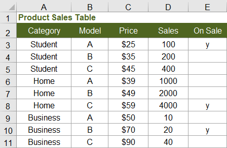
We’ll start off by using a product sales table to demonstrate a few different SUMIF and COUNTIF formulas. I’ve listed a few of these examples below. To see these formulas in action and try them out yourself, you can download the example file below:
Download the Example File (SumIf-CountIf.xlsx)
Criteria are Text Values
Example: Sum of Sales where Category equals «student»
=SUMIF(category_range,"student",sales_range)
NOTE This formula will also match «Student» because the SUMIF family of functions are not case-sensitive. You can use wildcard characters within the text string, such as «?s*» to match values where the second letter is s.
Not Equal To (<>)
Example: Sum of Sales where Model is NOT equal to «B»
=SUMIF(model_range,"<>B",sales_range)
Example: Sum of Sales where Category does NOT contain the letter «u»
=SUMIF(category_range,"<>*u*",sales_range)
Criteria is an Alphabetical Text Comparison
Example: Sum of Sales where Model is less than «C»
=SUMIF(model_range,"<C",sales_range)
Criteria is a Numeric Comparison
Example: Number of products priced over $40
=COUNTIF(price_range,">40")
NOTE When using numeric criteria, COUNTIF and SUMIF ignore text values. Numeric date values can be an exception to that (see below for date comparisons).
Criteria matches Blank Cells or Empty Cells
Example: Count of products where On Sale is blank
=COUNTIF(on_sale_range,"")
Criteria matches Non-Blank Cells
Example: Number of products on sale (where On Sale is not blank)
=COUNTIF(on_sale_range,"<>")
Criteria includes a Cell Reference
Example: Sum of Sales where Price is greater than the value in cell H3
=SUMIF(price_range,">"&H3,sales_range)
Criteria is In Another Cell
Example: Sum of Sales using the criteria defined in cell K9
=SUMIF(criteria_range,K9,sales_range)
NOTE This technique is useful when you want to allow the user to choose or enter different criteria or search strings.
The cell K9 could contain a value like «student» or «40» or a criteria string such as «>40» or «<>student»
Multiple Criteria
Example: Sum of Sales where Category = «student» AND Price > 30
=SUMIFS(sales_range,category_range,"student",price_range,">30")
Example: SUMIFS between two dates
=SUMIFS(sum_range,date_range,">=1/1/2017",date_range,"<1/31/2017")
NOTE The SUMIFS, COUNTIFS, and AVERAGEIFS functions are used for multiple AND conditions. Formulas for OR conditions are a bit more tricky (see below).
2) Using Dates as Criteria
When using dates as criteria for the COUNTIF and SUMIF functions, Excel does some interesting things, depending on whether you are using «=» or «<» as the criteria and whether the dates in the criteria range are stored as numeric date values or text values.
Remember: Date values are stored in Excel as sequential numbers starting with 1 for 1/1/1900. The cell formatting may display the date in different ways, but COUNTIF and SUMIF comparisons are based on the value stored in the cell, not the way a cell is formatted. That is a good, because we normally want to compare dates and numbers without having to worry about how they are formatted.
Criteria is a Date
=COUNTIF(criteria_range,"=3/1/17")
When using criteria such as «=3/1/17» or «Mar 1, 2017», Excel will recognize the criteria as a date and will count all date values in the criteria_range matching that date. Excel will ALSO count recognized dates stored as text values in the criteria_range, such as «March 1, 2017» and «3/1/2017» (but not «March 1st, 2017» because Excel doesn’t recognize it as a date).
Criteria is Greater or Less than a Date
=COUNTIF(criteria_range,">3/1/17")
When using <, >, <=, or >=, Excel still recognizes the criteria as a date, but it does not convert text values in the criteria_range to date values.
Comparison to TODAY
You can use the TODAY function to make comparisons based on the current date, like this:
=SUMIF(date_range,"<"&TODAY(),sum_range)
3) SUMIFS Example: Income and Expense Report
SUMIFS is very useful in account registers, budgeting, and money management spreadsheets for summarizing expenses by category and between two dates.
The SUMIFS example below sums the Amount column with 3 criteria: (1) the Category matches «Fuel», (2) the Date is greater than or equal to the start date, and (3) the Date is less than or equal to the end date.
=SUMIFS(amount_range, category_range, "Fuel", date_range, ">=1/1/2018", date_range, "<=1/31/2018")
The following screenshot shows an example from the download file:
4) SUMIF and COUNTIF Between Two Numbers (1 < x < 4)
COUNTIFS and SUMIFS can easily handle a condition such as 1 < x < 4 (which means x > 1 AND x < 4). However, if you are trying to make a spreadsheet compatible with older versions of Excel, you can use COUNTIF or SUMIF by subtracting the results of the condition x <= 1 from the results of the condition x < 4.
| Condition | Formula using COUNTIFS |
|---|---|
| 1 < x < 4 | =COUNTIFS(range,»>1″,range,»<4″) |
| Condition | Formula using only COUNTIF |
| 1 < x < 4 | =COUNTIF(range,»<4″) — COUNTIF(range,»<=1″) |
| 1 <= x < 4 | =COUNTIF(range,»<4″) — COUNTIF(range,»<1″) |
| 1 < x <= 4 | =COUNTIF(range,»<=4″) — COUNTIF(range,»<=1″) |
| 1 <= x <= 4 | =COUNTIF(range,»<=4″) — COUNTIF(range,»<1″) |
A common need for these formulas is to sum values between two dates. Remember that date values are stored as numbers.
Example: SUMIF between two dates ( 1/1/2017 <= date <= 1/31/2017 )
=SUMIF(sum_range,date_range,"<=1/31/2017")-SUMIF(sum_range,date_range,"<1/1/2017")
5) SUMIF and COUNTIF with OR Conditions
COUNTIFS and SUMIFS handle multiple AND conditions, but OR conditions such as X<2 OR X>3 are usually easier to handle by evaluating each condition separately and then adding the results. The two formulas below do essentially the same thing.
| Condition | Formula |
|---|---|
| x < 2 or 3 < x | =COUNTIF(range,»<2″) + COUNTIF(range,»>3″) |
| x < 2 or 3 < x | =SUM(COUNTIF(range,{«<2″,»>3″})) |
To avoid double-counting cells, the conditions must not overlap. For example, the condition «=*e*» would overlap with the condition «=yes». The condition «<40» would overlap with the condition «>20». If the conditions overlap, you may end up counting or adding a value twice. If there is a possibility of conditions overlapping, then you may need to use a SUMPRODUCT formula as explained below.
Use SUMPRODUCT for overlapping OR conditions
The key to avoid double-counting is to recognize that FALSE+FALSE=0 and TRUE+FALSE=1 and TRUE+TRUE=2. This means that for a logical OR condition to be true, we can check whether the sum of two or more conditions is > 0.
Sum of Sales where Model is equal to A or B.
=SUMPRODUCT(sales,1*( ((model="A")+(model="B"))>0 ))
Sum of Sales where Model = «A» or Price > 45
=SUMPRODUCT(sales,1*( ((model="A")+(price>45))>0 ))
6) Case-Sensitive SUMIF and COUNTIF
The SUMIF family does not have a case-sensitive option, so we need to resort back to using array formulas or SUMPRODUCT. The FIND and EXACT functions both provide a way to do case-sensitive matches.
Sum of Sales where Category exactly matches «student» (case-sensitive)
=SUMPRODUCT(sales,1*EXACT(category,"student"))
Sum of Sales where Category contains «Stu» (case-sensitive)
=SUMPRODUCT(sales,1*ISNUMBER(FIND("Stu",category)))
7) MAXIF or MINIF Formula
MAXIFS and MINIFS are new Excel functions available in the latest releases (Excel for Microsoft 365, Excel 2019). Their syntax is similar to SUMIFS, allowing you to use multiple criteria.
Older versions of Excel do not have the MAXIFS or MINIFS functions, but you can use an array formula like this (remember to press Ctrl+Shift+Enter):
Example: Find the maximum Price where Model = «A»
(array formula) =MAX(IF(model_range="A",price_range,""))
Summary of Different Criteria Types
| CRITERIA TYPE | EXAMPLE | MATCHES … |
|---|---|---|
| Text Value | «yes» or «=yes» | «yes» or «Yes» (not case-sensitive), the equal sign is optional |
| Text Value with Wildcards | «=?s*» | text values where the second letter is «s» or «S» |
| Alphabetical Text Comparison | «<C» | text values alphabetically less than «C» |
| Equal to a Numeric Value | 20 or «=20» | numeric values equal to 20 |
| Less than or Equal to | «<=20» | numeric values less than or equal to 20 |
| Greater than or Equal to | «>=20» | numeric values greater than or equal to 20 |
| Not Equal to | «<>0» | values not equal to the value 0 |
| Non-Blank | «<>» | values that are not blank (formulas returning «» are not blank) |
| Blank or Empty | «» | values that are blank and formulas that return «» |
| Equal to a Cell Value | A42 or «=»&A42 | values equal to the value in cell A42 |
| Comparison to a Cell Value | «>»&A42 | values greater than the value in cell A42 |
| Equal to a Date | «=3/1/17» | date values equal to 3/1/17 as well as text values such as «3/1/17» or «Mar 1, 2017» |
| < or > a Date | «>1/1/2017» | date values greater than 1/1/2017 (text values are ignored) |
Some criteria, such as case-sensitive matches, may only be possible with array formulas or SUMPRODUCT.
You don’t use the functions AND, NOT, OR, ISBLANK, ISNUMBER, ISERROR, or other similar functions as criteria for SUMIF and COUNTIF. However, you can use these functions within a SUMPRODUCT formula (but that isn’t within the scope of this article).
9) Other Notes
- Comparisons are based on the value stored in the cell, not on how the cell is formatted.
- Error values in both the sum_range and criteria_range are ignored.
- SUMIFS and COUNTIFS formulas are generally faster than their SUMPRODUCT or array formula counterparts.
- The sum_range and criteria_range arguments can be references (e.g. A2:A42), named ranges or formulas that return a range (such as INDEX, OFFSET, or INDIRECT).
- Normally, you’ll want the sum_range and criteria_range to be the same length. See the documentation on the Microsoft sites (referenced below) for information about what happens when the sum_range and criteria_range are not the same length.
- The COUNTIF and SUMIF criteria can be a range (e.g. A2:A3) if you enter the formula as an array formula using Ctrl+Shift+Enter.
- The COUNTIF and SUMIF criteria can be a list such as {«>1″,»<4»}, but functions return an array containing results for the separate conditions, not a sum of both conditions (it is not the same as COUNTIFS or SUMIFS).
Some Templates that Use SUMIF
- Invoice Tracker — Uses SUMIF to create an Aging table that shows unpaid invoices past 30 days, 60 days, etc.
- Account Register — Uses a cumulative SUMIF formula to show the current account balance within the register.
- Weekly Money Manager — Uses SUMIF to show actual spending within a budget report.
- Checkbook Register — Uses SUMIF to show the current cleared balance based on whether the reconcile column contains «r» or «c».
References
- Spreadsheet Tips Workbook — vertex42.com — by Jon Wittwer and Brent Weight
- SUMIF Function — support.office.com — The official documentation of the SUMIF function.
- SUMIFS Function — support.office.com — The official documentation of the SUMIFS function.
- COUNTIF Function — support.office.com — The official documentation of the COUNTIF function.
- COUNTIFS Function — support.office.com — The official documentation of the COUNTIFS function.
- SUMIFS With Multiple Criteria and OR Logic — at exceljet.net — Describes how the function works when you use an array for the criteria such as {«=A»,»=B»}.
Learning Microsoft Excel is all about adding more and more formulas and functions to your toolbelt. Combine enough of these, and you can do practically anything with a spreadsheet.
In this tutorial, you’ll learn how to use three powerful Excel formulas: SUMIF, COUNTIF, and AVERAGEIF.
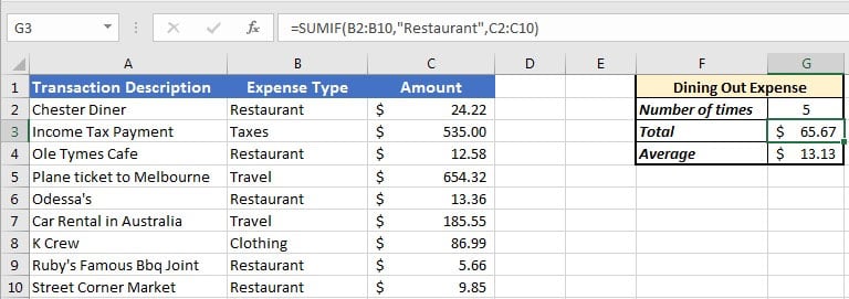


In the screenshot above, you can see that we have a list of transactions on the left side. If I want to keep an eye on my spending, I can use these three formulas to monitor it.
On the right side, the Dining Out Expense box uses the three formulas to help me track my expenses:
- COUNTIF — Used to count the number of times that «Restaurant» appears in the list.
- SUMIF — Calculates the total expense for items labeled «Restaurant.»
- AVERAGIEF — Averages out all of my «Restaurant» expenses in the list.
More generically, here’s what each of those formulas do for you, and how you might use them to your advantage:
- SUMIF — Add values if a condition is met, such as adding up all purchases from one category.
- COUNTIF — Count up the number of items that meet a condition, such as counting the number of times a name appears in a list.
- AVERAGEIF — Conditionally average values; for instance, you could average your grades for only exams.
These formulas allow you to add logic to your spreadsheet. Let’s look at how to use each formula.
COUNTIF, SUMIF, and AVERAGEIF in Excel (Quick Video Tutorial)
Screencasts are one of the best ways to watch and learn a new skill, including getting started with these three key formulas in Microsoft Excel. Check out the video below to watch how I work in Excel. Make sure and download the free example workbook to use with this tutorial.
If you prefer to learn with written, step-by-step instructions, keep reading. I’ll share tips for how to use these formulas and ideas for why they’re useful.
How to Use SUMIF in Excel
Use the tab titled SUMIF in the free example workbook for this section of the tutorial.
Think of SUMIF as a way to add values that meet a rule. We can add up a list of values that are from a certain category, or all values greater than or less than a specific amount.
Here’s how the SUMIF formula works:
=SUMIF(Cells to check, what to check for, Sum of cells that meet the rules)
Let’s go back to my restaurant expense example to learn the SUMIF formula. Below, I show a list of my transactions for the month.
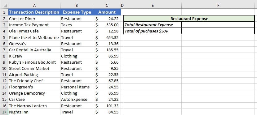


I want to know two things:
- The total of what I spent at restaurants for the month.
- All purchases greater than $50 for the month, from any category.
Instead of manually adding data up, we can write two SUMIF formulas to automate the process. I’ll put the results in the green Restaurant Expense box on the right side. Let’s look at how.
Total Restaurant Expense
To find my total restaurant expense, I’ll sum up all values with the expense type of «Restaurant», which is in column B.
Here’s the formula I’ll use for this example:
=SUMIF(B2:B17,"Restaurant",C2:C17)
Notice that each section is separated by a comma. This formula does three key things:
- Looks at what’s in cells B2 to B17 for the category of expense
- Uses «Restaurant» for the criteria of what to sum up
- Uses the values in cells C2 to C17 to total up the amounts
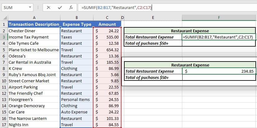


When I press enter, Excel calculates the total of my restaurant expenses. Using SUMIF, it’s easy to create these quick statistics to help you monitor data of certain types.
Purchases Greater Than $50
We’ve checked for a specific category, but now let’s sum up all values that are greater than an amount from any category. In this case, I want to find all purchases that were more than $50.
Let’s write a simple formula to find the sum of all purchases greater than $50:
=SUMIF(C2:C17,">50")
In this case, the formula is a bit simpler: since we’re summing up the same values that we’re testing (C2 to C17), we just need to specify those cells. Then, we’ll add a comma and «>50» to only sum values greater than $50.


This example uses a greater than sign, but for bonus points: try to sum up all small purchases, such as all purchases $20 or less.
How to Use COUNTIF in Excel
Use the tab titled COUNTIF in the free example workbook for this section of the tutorial.
While SUMIF is used to add values that meet a certain condition, COUNTIF will count up the number of times something appears in a given set of data.
Here’s the general format for the COUNTIF formula:
=COUNTIF(cells to count, criteria to count)
Using the same set of data, let’s count two key pieces of information:
- The number of clothing purchases I made in a month
- The number of purchases $100 or greater
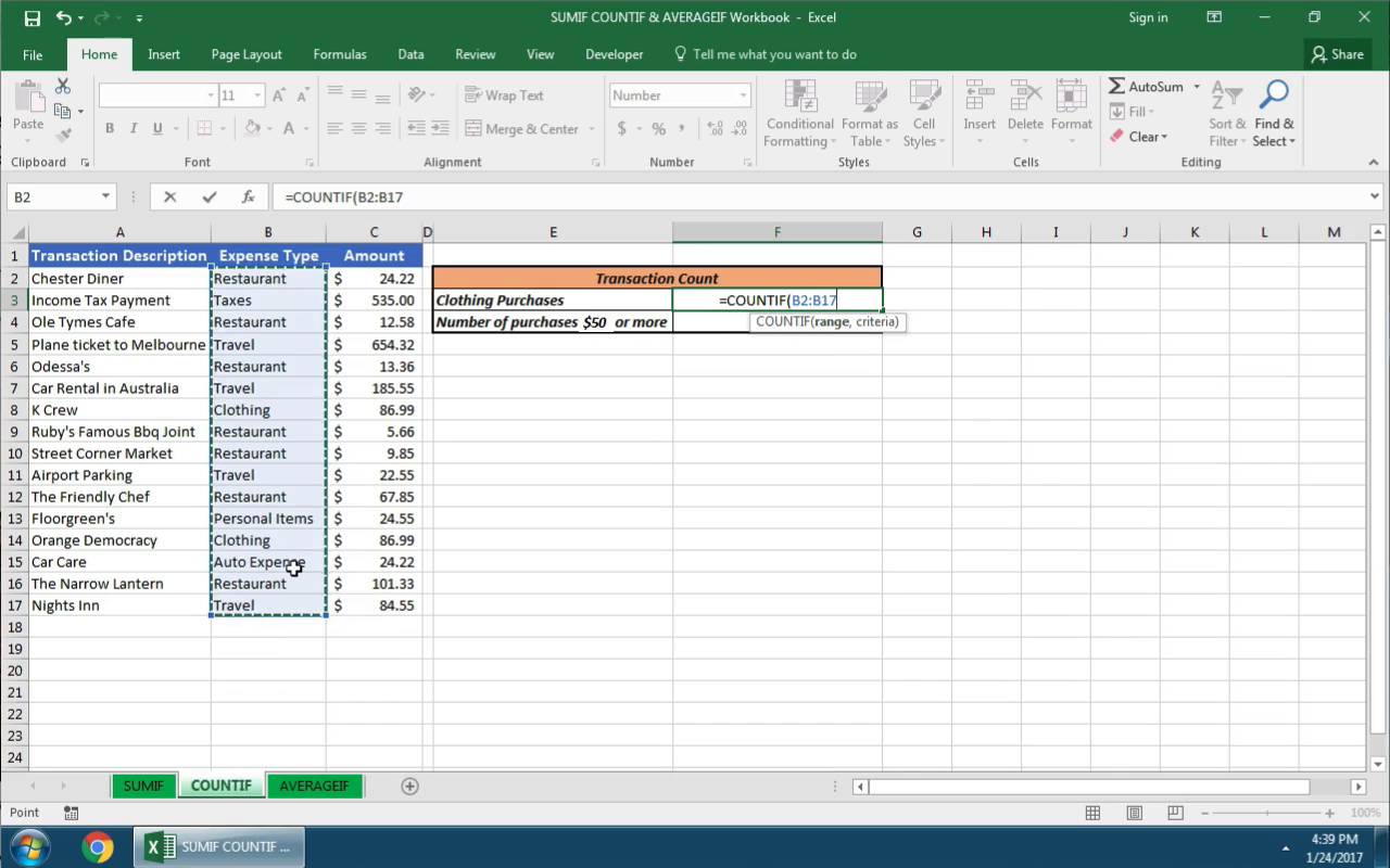
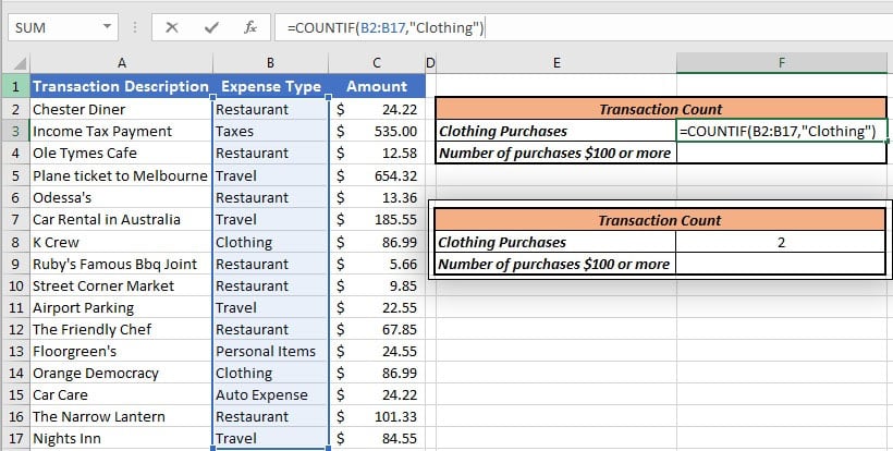
Number of Clothing Purchases
My first COUNTIF will look at the expense type and count up the number of «Clothing» purchases in my transactions.
The final formula will be:
=COUNTIF(B2:B17,"Clothing")
That formula looks at the «Expense Type» column, counts up the number of times it sees clothing, and counts them. The result is 2.


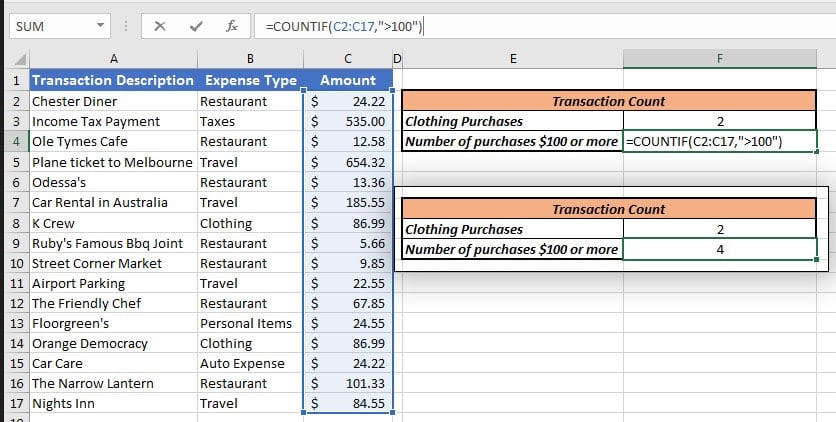
Number of $100+ Purchases
Now, let’s count the number of transactions that were $100 or greater in my list.
Here’s the formula I’ll use:
=COUNTIF(C2:C17,">100")
This is a simple, two part formula: simply point Excel to the list of data to count, and the rule to count. In this case, we’re checking cells C2 to C17, for all values greater than $100.


How to Use AVERAGEIF in Excel
Use the tab titled AVERAGEIF in the free example workbook for this section of the tutorial.
Last up, let’s look at how to use an AVERAGEIF formula. By now, it should be no surprise that AVERAGEIF can be used to average specific values, based on a condition that we’ll give Excel.
The format for an AVERAGEIF formula is:
=AVERAGEIF(Cells to check, what to check for, Average of cells that meet the rules)
The format of the AVERAGEIF formula is most similar to the SUMIF formula.
Let’s use the AVERAGEIF formula to calculate two key stats about my spending:
- The average of my restaurant expenses.
- The average of all expenses less than $25.
Average of Restaurant Purchases
To average my restaurant expenses, I’ll write an AVERAGEIF formula to average all amounts based on the category.
=AVERAGEIF(B2:B17,"Restaurant",C2:C17)
There are three parts to this formula, each separated by a comma:
- B2:B17 specifies the cells to check a condition for. Since the expense type is specified in this column.
- «Restaurant» gives the formula something to look for.
- Finally, C2:C17 are the cells to average out in our calculation.
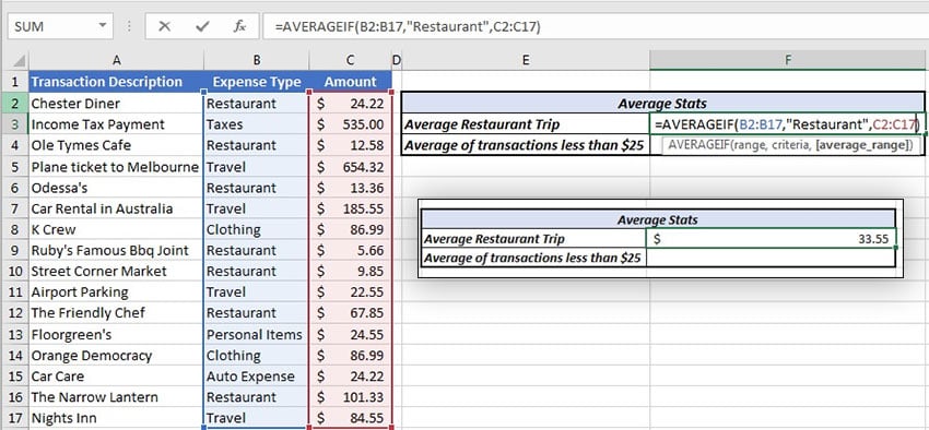


At the end, Excel averages out the expense of my restaurant trips. I’ve given it that formula.
You can also try out this formula by replacing «Restaurant» with another category, like «Clothing.»
Average of Expenses Less than $25
If I’m keeping an eye on my smaller purchases and want to know my average, I can write an AVERAGEIF for all purchases less than an amount.
Here’s the formula that I’ll use to do that:
=AVERAGEIF(C2:C17,"<25")
This simple formula just checks the values in column C, and averages all values greater than $25.


Recap and Keep Learning
In this tutorial, you learned how to use three conditional math formulas to review your data. Whether you’re summing, counting, or averaging data, these functions are advanced Excel skills you can put to good use.
For all of the «IF» formulas in this tutorial, the key takeaway is that you can apply conditions to your calculations in Excel.
Learning begets learning. Here are three more Excel tutorials to keep growing:
- In addition to COUNTIF, SUMIF, and AVERAGEIF, there are also general «IF» statements that can be used for other conditions. Check out our tutorial on How to Use Simple IF Statements.
- Learn to use Excel Dates and Times in conjunction with these formulas to work with values based upon date.
- The Excel VLOOKUP function can be used to match values from multiple lists. Learn more about How to Use the Excel VLOOKUP Function in this tutorial.
Can you think of other ways to use these formulas to add logic and conditions to your spreadsheet? Let me know with a comment below.
Count how often a value occurs
Excel for Microsoft 365 Excel for Microsoft 365 for Mac Excel for the web Excel 2021 Excel 2021 for Mac Excel 2019 Excel 2019 for Mac Excel 2016 Excel 2016 for Mac Excel 2013 Excel 2010 Excel 2007 Excel for Mac 2011 More…Less
Suppose you want to find out how many times particular text or a number value occurs in a range of cells. For example:
-
If a range, such as A2:D20, contains the number values 5, 6, 7, and 6, then the number 6 occurs two times.
-
If a column contains «Buchanan», «Dodsworth», «Dodsworth», and «Dodsworth», then «Dodsworth» occurs three times.
There are several ways to count how often a value occurs.
Use the COUNTIF function to count how many times a particular value appears in a range of cells.

For more information, see COUNTIF function.
The COUNTIFS function is similar to the COUNTIF function with one important exception: COUNTIFS lets you apply criteria to cells across multiple ranges and counts the number of times all criteria are met. You can use up to 127 range/criteria pairs with COUNTIFS.
The syntax for COUNTIFS is:
COUNTIFS(criteria_range1, criteria1, [criteria_range2, criteria2],…)
See the following example:

To learn more about using this function to count with multiple ranges and criteria, see COUNTIFS function.
Let’s say you need to determine how many salespeople sold a particular item in a certain region or you want to know how many sales over a certain value were made by a particular salesperson. You can use the IF and COUNT functions together; that is, you first use the IF function to test a condition and then, only if the result of the IF function is True, you use the COUNT function to count cells.
Notes:
-
The formulas in this example must be entered as array formulas.
-
If you have a current version of Microsoft 365, then you can simply enter the formula in the top-left-cell of the output range, then press ENTER to confirm the formula as a dynamic array formula.
-
If you have opened this workbook in Excel for Windows or Excel 2016 for Mac and newer versions, and want to change the formula or create a similar formula, press F2, and then press Ctrl+Shift+Enter to make the formula return the results you expect. In earlier versions of Excel for Mac, use
+Shift+Enter.
-
-
For the example formulas to work, the second argument for the IF function must be a number.
 +Shift+Enter.
To learn more about these functions, see COUNT function and IF function.
In the examples that follow, we use the IF and SUM functions together. The IF function first tests the values in some cells and then, if the result of the test is True, SUM totals those values that pass the test.
Notes: The formulas in this example must be entered as array formulas.
-
If you have a current version of Microsoft 365, then you can simply enter the formula in the top-left-cell of the output range, then press ENTER to confirm the formula as a dynamic array formula.
-
If you have opened this workbook in Excel for Windows or Excel 2016 for Mac and newer versions, and want to change the formula or create a similar formula, press F2, and then press Ctrl+Shift+Enter to make the formula return the results you expect. In earlier versions of Excel for Mac, use
+Shift+Enter.
Example 1

The above function says if C2:C7 contains the values Buchanan and Dodsworth, then the SUM function should display the sum of records where the condition is met. The formula finds three records for Buchanan and one for Dodsworth in the given range, and displays 4.
Example 2

The above function says if D2:D7 contains values lesser than $9000 or greater than $19,000, then SUM should display the sum of all those records where the condition is met. The formula finds two records D3 and D5 with values lesser than $9000, and then D4 and D6 with values greater than $19,000, and displays 4.
Example 3

The above function says if D2:D7 has invoices for Buchanan for less than $9000, then SUM should display the sum of records where the condition is met. The formula finds that C6 meets the condition, and displays 1.
You can use a PivotTable to display totals and count the occurrences of unique values. A PivotTable is an interactive way to quickly summarize large amounts of data. You can use a PivotTable to expand and collapse levels of data to focus your results and to drill down to details from the summary data for areas that are of interest to you. In addition, you can move rows to columns or columns to rows («pivoting») to see a count of how many times a value occurs in a PivotTable. Let’s look at a sample scenario of a Sales spreadsheet, where you can count how many sales values are there for Golf and Tennis for specific quarters.
-
Enter the following data in an Excel spreadsheet.
-
Select A2:C8
-
Click Insert > PivotTable.
-
In the Create PivotTable dialog box, click Select a table or range, then click New Worksheet, and then click OK.
An empty PivotTable is created in a new sheet.
-
In the PivotTable Fields pane, do the following:
-
Drag Sport to the Rows area.
-
Drag Quarter to the Columns area.
-
Drag Sales to the Values area.
-
Repeat step c.
The field name displays as SumofSales2 in both the PivotTable and the Values area.
At this point, the PivotTable Fields pane looks like this:
-
In the Values area, click the dropdown next to SumofSales2 and select Value Field Settings.
-
In the Value Field Settings dialog box, do the following:
-
In the Summarize value field by section, select Count.
-
In the Custom Name field, modify the name to Count.
-
Click OK.
-
The PivotTable displays the count of records for Golf and Tennis in Quarter 3 and Quarter 4, along with the sales figures.
-


Need more help?
You can always ask an expert in the Excel Tech Community or get support in the Answers community.
See Also
Overview of formulas in Excel
How to avoid broken formulas
Find and correct errors in formulas
Excel keyboard shortcuts and function keys
Excel functions (alphabetical)
Excel functions (by category)
Need more help?
I wanted to continue building on my popular series on how to use IF statements and nested IF statements with “and, or, not” in Excel by discussing two additional and very useful functions called countif and sumif. Surprisingly, they’re not as widely used as you’d expect, and sometimes knowing which to use is a bit confusing.
Countif is a function that will count (as in 1, 2, 3…) the number of entries within a range if certain criteria are met, and the data within each entry can be text or numbers.
Sumif, on the other hand, is a function that will add the total number of numerical entries within a range if certain criteria are met. This means that sumif only works with numbers when adding up figures, so if your range includes any text, those will be ignored. Let’s walk through a simple example.
Suppose you have the following simple table of sales by type and # for each year from 2003-2009:

And what you’d like to know is how many sales of each type (in your store vs. by phone vs. online) were done in total. Countif will help you figure that out quickly. First, let’s enter the type of sale we’re interested in in a column to the right:

Next, we’ll type in the “countif” function. As you can see, countif takes two inputs, the range you’re interested in and the criteria that need to be met:

In our case, the data (store type) is in column B, so we input that into the first part of the countif function:

Next, we want each entry to be counted only if the type of sale was “store”, or what we’ve typed into cell E2:

Note that if we hadn’t typed in “store” in E2, we could type it directly into the function like this:
=countif(B2:B20, “store”)
By the way, remember to always put quotation marks (“”) around the criteria when working with text!
Either way, once we close the parenthesis and hit , we immediately get the result. There were 7 sales from 2003-2009 that took place at the store (one for each year).

Repeating the same thing for “telephone”:

We find the same result — 7 sales. Now let’s check “online”:

Turns out we had less online sales (maybe because we didn’t launch a website that accepted sales until 2005):

That’s fine and dandy, but not particularly useful info. How about if we wanted to know the total number of sales by type for the entire period? In that case, we’d want to use the sumif function.
For “store” sales, we’d enter in sumif and the appropriate inputs as
follows. First, sumif takes in slightly different inputs than countif.

The first input is the range that you’re interested in, very similar to countif:

The second input is the criteria, which in this case is also identical to what we put in for countif above:

But sumif also takes one additional argument: the range to be summed. In this case, we want to know the total number of sales, which is in column C:

Closing out the parenthesis, we find that we had 211 total sales in the store from 2003-2009:

Again, let’s repeat the same thing to find the total number of telephone sales:

…and online sales:

See the difference between what countif gives and what sumif gives?
Note that sumif can also take in different criteria. Let’s suppose we wanted to know the total number of sales that have taken place starting in 2008, regardless of type. To do this, we could make our range the year, found in column A:

and then add in the criteria of “>= 2008”:

Finally, we again want to sum up the total number of sales, which is in column C:

Closing out our final parenthesis, we get that we have had a total of 141 sales from 2008-2009:

Finally, just a quick example here will show what happens if you put in non-numerical data to sum using the sumif function. Let’s change the number of store sales in 2008 from “37” to “nonsense” and see what happens:

Notice how the calculations automatically ignore that entry, and the total number of store sales and the total number of sales since 2008 both drop by 37.
That’s it for now. A quick intro tutorial to using countif and sumif. Like most other Excel functions, these can get as complicated as you’d like (at the expense of readability), so always try to keep it as simple as possible.
***************************************************
Look Good at Work and Become Indispensable Become an Excel Pro and Impress Your Boss

***************************************************