
Excel for Microsoft 365 Excel 2021 Excel 2019 Excel 2016 Excel 2013 Excel 2010 Excel 2007 More…Less
To count numbers or dates that meet a single condition (such as equal to, greater than, less than, greater than or equal to, or less than or equal to), use the COUNTIF function. To count numbers or dates that fall within a range (such as greater than 9000 and at the same time less than 22500), you can use the COUNTIFS function. Alternately, you can use SUMPRODUCT too.
Example
Note: You’ll need to adjust these cell formula references outlined here based on where and how you copy these examples into the Excel sheet.
|
1 |
A |
B |
|---|---|---|
|
2 |
Salesperson |
Invoice |
|
3 |
Buchanan |
15,000 |
|
4 |
Buchanan |
9,000 |
|
5 |
Suyama |
8,000 |
|
6 |
Suyma |
20,000 |
|
7 |
Buchanan |
5,000 |
|
8 |
Dodsworth |
22,500 |
|
9 |
Formula |
Description (Result) |
|
10 |
=COUNTIF(B2:B7,»>9000″) |
The COUNTIF function counts the number of cells in the range B2:B7 that contain numbers greater than 9000 (4) |
|
11 |
=COUNTIF(B2:B7,»<=9000″) |
The COUNTIF function counts the number of cells in the range B2:B7 that contain numbers less than 9000 (4) |
|
12 |
=COUNTIFS(B2:B7,»>=9000″,B2:B7,»<=22500″) |
The COUNTIFS function (available in Excel 2007 and later) counts the number of cells in the range B2:B7 greater than or equal to 9000 and are less than or equal to 22500 (4) |
|
13 |
=SUMPRODUCT((B2:B7>=9000)*(B2:B7<=22500)) |
The SUMPRODUCT function counts the number of cells in the range B2:B7 that contain numbers greater than or equal to 9000 and less than or equal to 22500 (4). You can use this function in Excel 2003 and earlier, where COUNTIFS is not available. |
|
14 |
Date |
|
|
15 |
3/11/2011 |
|
|
16 |
1/1/2010 |
|
|
17 |
12/31/2010 |
|
|
18 |
6/30/2010 |
|
|
19 |
Formula |
Description (Result) |
|
20 |
=COUNTIF(B14:B17,»>3/1/2010″) |
Counts the number of cells in the range B14:B17 with a data greater than 3/1/2010 (3) |
|
21 |
=COUNTIF(B14:B17,»12/31/2010″) |
Counts the number of cells in the range B14:B17 equal to 12/31/2010 (1). The equal sign is not needed in the criteria, so it is not included here (the formula will work with an equal sign if you do include it («=12/31/2010»). |
|
22 |
=COUNTIFS(B14:B17,»>=1/1/2010″,B14:B17,»<=12/31/2010″) |
Counts the number of cells in the range B14:B17 that are between (inclusive) 1/1/2010 and 12/31/2010 (3). |
|
23 |
=SUMPRODUCT((B14:B17>=DATEVALUE(«1/1/2010»))*(B14:B17<=DATEVALUE(«12/31/2010»))) |
Counts the number of cells in the range B14:B17 that are between (inclusive) 1/1/2010 and 12/31/2010 (3). This example serves as a substitute for the COUNTIFS function that was introduced in Excel 2007. The DATEVALUE function converts the dates to a numeric value, which the SUMPRODUCT function can then work with. |
Need more help?
Содержание
- COUNT function
- Syntax
- Remarks
- Example
- COUNTIF function
- Examples
- Common Problems
- Best practices
- Need more help?
- Count function in excel with if function
- Table of contents
- 1. Use IF + COUNTIF to evaluate multiple conditions
- 1.1 Explaining formula in cell D3
- Step 1 — COUNTIF function syntax
- Step 2 — Populate COUNTIF function arguments
- Step 3 — Evaluate COUNTIF function
- Step 4 — IF function syntax
- Step 5 — Populate IF function arguments
- Step 6 — Evaluate IF function
- 2. Use IF + COUNTIF to evaluate multiple conditions and calculate different outcomes
- 2.1 Explaining formula
- Step 1 — Check if the value matches any of the conditions
- Step 2 — IF function
- Step 3 — Calculate the relative position of a lookup value
- Step 3 — Get value
- Step 4 — Add values
- Get Excel *.xlsx file
- Logic category
- Functions in this article
- Excel formula categories
- Excel categories
- 3 Responses to “Use IF + COUNTIF to evaluate multiple conditions”
- Leave a Reply
- How to comment
- Ways to count values in a worksheet
- Download our examples
- In this article
- Simple counting
- Video: Count cells by using the Excel status bar
- Use AutoSum
- Add a Subtotal row
- Count cells in a list or Excel table column by using the SUBTOTAL function
- Counting based on one or more conditions
- Video: Use the COUNT, COUNTIF, and COUNTA functions
- Count cells in a range by using the COUNT function
- Count cells in a range based on a single condition by using the COUNTIF function
- Count cells in a column based on single or multiple conditions by using the DCOUNT function
- Count cells in a range based on multiple conditions by using the COUNTIFS function
- Count based on criteria by using the COUNT and IF functions together
- Count how often multiple text or number values occur by using the SUM and IF functions together
- Count cells in a column or row in a PivotTable
- Counting when your data contains blank values
- Count nonblank cells in a range by using the COUNTA function
- Count nonblank cells in a list with specific conditions by using the DCOUNTA function
- Count blank cells in a contiguous range by using the COUNTBLANK function
- Count blank cells in a non-contiguous range by using a combination of SUM and IF functions
- Counting unique occurrences of values
- Count the number of unique values in a list column by using Advanced Filter
- Count the number of unique values in a range that meet one or more conditions by using IF, SUM, FREQUENCY, MATCH, and LEN functions
- Special cases (count all cells, count words)
- Count the total number of cells in a range by using ROWS and COLUMNS functions
- Count words in a range by using a combination of SUM, IF, LEN, TRIM, and SUBSTITUTE functions
- Displaying calculations and counts on the status bar
- Need more help?
COUNT function
The COUNT function counts the number of cells that contain numbers, and counts numbers within the list of arguments. Use the COUNT function to get the number of entries in a number field that is in a range or array of numbers. For example, you can enter the following formula to count the numbers in the range A1:A20: =COUNT(A1:A20). In this example, if five of the cells in the range contain numbers, the result is 5.

Syntax
The COUNT function syntax has the following arguments:
value1 Required. The first item, cell reference, or range within which you want to count numbers.
value2, . Optional. Up to 255 additional items, cell references, or ranges within which you want to count numbers.
Note: The arguments can contain or refer to a variety of different types of data, but only numbers are counted.
Arguments that are numbers, dates, or a text representation of numbers (for example, a number enclosed in quotation marks, such as «1») are counted.
Logical values and text representations of numbers that you type directly into the list of arguments are counted.
Arguments that are error values or text that cannot be translated into numbers are not counted.
If an argument is an array or reference, only numbers in that array or reference are counted. Empty cells, logical values, text, or error values in the array or reference are not counted.
If you want to count logical values, text, or error values, use the COUNTA function.
If you want to count only numbers that meet certain criteria, use the COUNTIF function or the COUNTIFS function.
Example
Copy the example data in the following table, and paste it in cell A1 of a new Excel worksheet. For formulas to show results, select them, press F2, and then press Enter. If you need to, you can adjust the column widths to see all the data.
Источник
COUNTIF function
Use COUNTIF, one of the statistical functions, to count the number of cells that meet a criterion; for example, to count the number of times a particular city appears in a customer list.
In its simplest form, COUNTIF says:
=COUNTIF(Where do you want to look?, What do you want to look for?)
The group of cells you want to count. Range can contain numbers, arrays, a named range, or references that contain numbers. Blank and text values are ignored.
A number, expression, cell reference, or text string that determines which cells will be counted.
For example, you can use a number like 32, a comparison like «>32», a cell like B4, or a word like «apples».
COUNTIF uses only a single criteria. Use COUNTIFS if you want to use multiple criteria.
Examples
To use these examples in Excel, copy the data in the table below, and paste it in cell A1 of a new worksheet.
Counts the number of cells with apples in cells A2 through A5. The result is 2.
Counts the number of cells with peaches (the value in A4) in cells A2 through A5. The result is 1.
Counts the number of apples (the value in A2), and oranges (the value in A3) in cells A2 through A5. The result is 3. This formula uses COUNTIF twice to specify multiple criteria, one criteria per expression. You could also use the COUNTIFS function.
Counts the number of cells with a value greater than 55 in cells B2 through B5. The result is 2.
Counts the number of cells with a value not equal to 75 in cells B2 through B5. The ampersand (&) merges the comparison operator for not equal to (<>) and the value in B4 to read =COUNTIF(B2:B5,»<>75″). The result is 3.
=COUNTIF(B2:B5,»>=32″)-COUNTIF(B2:B5,» ) or equal to (=) 32 and less than (
Common Problems
What went wrong
Wrong value returned for long strings.
The COUNTIF function returns incorrect results when you use it to match strings longer than 255 characters.
To match strings longer than 255 characters, use the CONCATENATE function or the concatenate operator &. For example, =COUNTIF(A2:A5,»long string»&»another long string»).
No value returned when you expect a value.
Be sure to enclose the criteria argument in quotes.
A COUNTIF formula receives a #VALUE! error when referring to another worksheet.
This error occurs when the formula that contains the function refers to cells or a range in a closed workbook and the cells are calculated. For this feature to work, the other workbook must be open.
Best practices
Be aware that COUNTIF ignores upper and lower case in text strings.
Criteria aren’t case sensitive. In other words, the string «apples» and the string «APPLES» will match the same cells.
Use wildcard characters.
Wildcard characters —the question mark (?) and asterisk (*)—can be used in criteria. A question mark matches any single character. An asterisk matches any sequence of characters. If you want to find an actual question mark or asterisk, type a tilde (
) in front of the character.
For example, =COUNTIF(A2:A5,»apple?») will count all instances of «apple» with a last letter that could vary.
Make sure your data doesn’t contain erroneous characters.
When counting text values, make sure the data doesn’t contain leading spaces, trailing spaces, inconsistent use of straight and curly quotation marks, or nonprinting characters. In these cases, COUNTIF might return an unexpected value.
For convenience, use named ranges
COUNTIF supports named ranges in a formula (such as =COUNTIF( fruit,»>=32″)-COUNTIF( fruit,»>85″). The named range can be in the current worksheet, another worksheet in the same workbook, or from a different workbook. To reference from another workbook, that second workbook also must be open.
Note: The COUNTIF function will not count cells based on cell background or font color. However, Excel supports User-Defined Functions (UDFs) using the Microsoft Visual Basic for Applications (VBA) operations on cells based on background or font color. Here is an example of how you can Count the number of cells with specific cell color by using VBA.
Need more help?
You can always ask an expert in the Excel Tech Community or get support in the Answers community.
Источник
Count function in excel with if function
The image above demonstrates a formula that matches a value to multiple conditions, if the condition is met the formula takes the value in a corresponding cell on the same row and adds a given number.
Table of contents
The COUNTIF function allows you to construct a small IF formula that carries out plenty of logical expressions.
Combining the IF and COUNTIF functions also let you have more than 254 logical expressions and the effort to type the formula is minimal.
1. Use IF + COUNTIF to evaluate multiple conditions
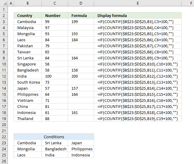
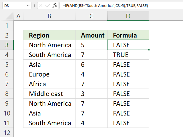
The example shown in the above picture checks if the country in cell B3 is equal to one of the countries in cell range B23:D25.
In other words, the COUNTIF function counts how many times a specific value is found in a cell range.
If the value exists at least once in the cell range the IF function adds 100 to the value in C3. If FALSE the formula returns a blank.
1.1 Explaining formula in cell D3
Step 1 — COUNTIF function syntax
The COUNTIF function calculates the number of cells that is equal to a condition.
Step 2 — Populate COUNTIF function arguments
range — A reference to all conditions: $B$23:$D$25
criteria — The value to match.
Step 3 — Evaluate COUNTIF function
and returns 1. The criteria value is found once in the array (bolded).
Step 4 — IF function syntax
The IF function returns one value if the logical test is TRUE and another value if the logical test is FALSE.
IF(logical_test, [value_if_true], [value_if_false])
Step 5 — Populate IF function arguments
IF(logical_test, [value_if_true], [value_if_false])
logical_test — True or False, the numerical equivalents are TRUE — 1 and False — 0 (zero). 1, in this case, is equal to TRUE.
[value_if_true] — C3+100, add 100 to value in cell C3.
Step 6 — Evaluate IF function
IF(COUNTIF($B$23:$D$25, B3), C3+100, «»)
and returns 199 in cell D3.
2. Use IF + COUNTIF to evaluate multiple conditions and calculate different outcomes
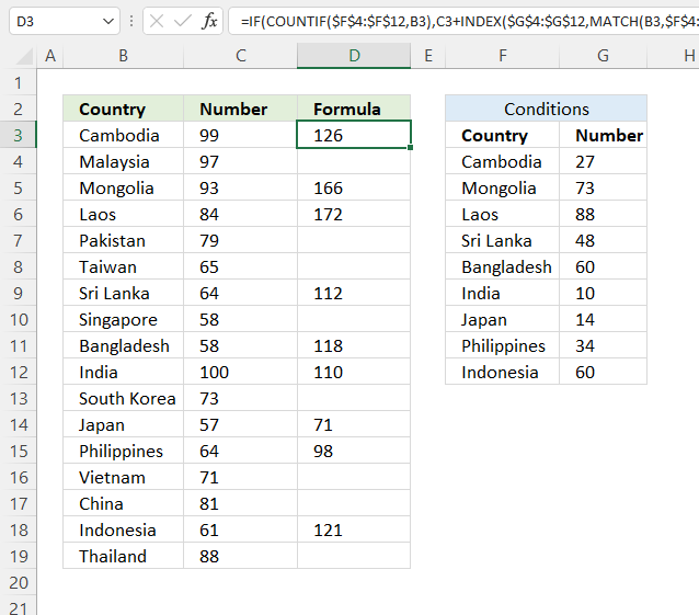
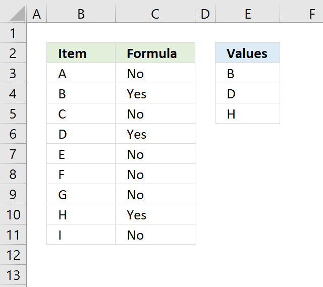
The image above demonstrates a formula in cell D3 that checks if the value in cell B3 matches any of the conditions specified in cell range F4:F12. If so, add the corresponding number in cell range G4:G12 to the number in cell C3.
Formula in cell D3:
2.1 Explaining formula
Step 1 — Check if the value matches any of the conditions
The COUNTIF function calculates the number of cells that is equal to a condition.
and returns 1. This means that there is one value that matches.
Step 2 — IF function
The IF function returns one value if the logical test is TRUE and another value if the logical test is FALSE.
IF(logical_test, [value_if_true], [value_if_false])
IF(COUNTIF($F$4:$F$12, B3), [value_if_true], [value_if_false])
IF(1, [value_if_true], [value_if_false])
[value_if_true] — C3+INDEX($G$4:$G$12, MATCH(B3, $F$4:$F$12,0))
Step 3 — Calculate the relative position of a lookup value
The MATCH function returns the relative position of an item in an array or cell reference that matches a specified value in a specific order.
MATCH(lookup_value, lookup_array, [match_type])
and returns 1. The lookup value is found at the first position in the array.
Step 3 — Get value
The INDEX function returns a value from a cell range, you specify which value based on a row and column number.
INDEX(array, [row_num], [column_num])
INDEX($G$4:$G$12, MATCH(B3, $F$4:$F$12,0))
Step 4 — Add values
The plus sign lets you add numbers in an Excel formula.
C3+INDEX($G$4:$G$12, MATCH(B3, $F$4:$F$12,0))
99 + 27 equals 126.
Get Excel *.xlsx file
Logic category
Functions in this article
Excel formula categories
Excel categories
3 Responses to “Use IF + COUNTIF to evaluate multiple conditions”
1. If item Count in Column-A have equal Count of the same item in corresponding Column-B, Result should be «Complete»
2. If item Count in Column-A have Count at least one in corresponding Column-B but less than Count in Column-A, Result should be «In progress»
3. If item Count in Column-A have no Count in corresponding Column-B, Result should be «Not Complete»
4. If there is no Count in Column-A and corresponding Column-B have no count, Result should be «Blank»
Please reply
If the marks of a student is less than 16 or his average is less than 50 he must be in D group.
How can i write this formula? Please write it for me
Please reply
If the marks of a student is less than 16 or his average is less than 50 he must be in D group.
How can i write this formula in table of contant? Please write it for me
Leave a Reply
How to add a formula to your comment
Insert your formula here.
Convert less than and larger than signs
Use html character entities instead of less than and larger than signs.
becomes >
How to add VBA code to your comment
[vb 1=»vbnet» language=»,»]
Put your VBA code here.
[/vb]
How to add a picture to your comment:
Upload picture to postimage.org or imgur
Paste image link to your comment.
Contact Oscar

You can contact me through this contact form
Источник
Ways to count values in a worksheet
Counting is an integral part of data analysis, whether you are tallying the head count of a department in your organization or the number of units that were sold quarter-by-quarter. Excel provides multiple techniques that you can use to count cells, rows, or columns of data. To help you make the best choice, this article provides a comprehensive summary of methods, a downloadable workbook with interactive examples, and links to related topics for further understanding.
Note: Counting should not be confused with summing. For more information about summing values in cells, columns, or rows, see Summing up ways to add and count Excel data.
Download our examples
You can download an example workbook that gives examples to supplement the information in this article. Most sections in this article will refer to the appropriate worksheet within the example workbook that provides examples and more information.
In this article
Simple counting
You can count the number of values in a range or table by using a simple formula, clicking a button, or by using a worksheet function.
Excel can also display the count of the number of selected cells on the Excel status bar. See the video demo that follows for a quick look at using the status bar. Also, see the section Displaying calculations and counts on the status bar for more information. You can refer to the values shown on the status bar when you want a quick glance at your data and don’t have time to enter formulas.
Video: Count cells by using the Excel status bar
Watch the following video to learn how to view count on the status bar.
Use AutoSum
Use AutoSum by selecting a range of cells that contains at least one numeric value. Then on the Formulas tab, click AutoSum > Count Numbers.

Excel returns the count of the numeric values in the range in a cell adjacent to the range you selected. Generally, this result is displayed in a cell to the right for a horizontal range or in a cell below for a vertical range.
Add a Subtotal row
You can add a subtotal row to your Excel data. Click anywhere inside your data, and then click Data > Subtotal.
Note: The Subtotal option will only work on normal Excel data, and not Excel tables, PivotTables, or PivotCharts.

Also, refer to the following articles:
Count cells in a list or Excel table column by using the SUBTOTAL function
Use the SUBTOTAL function to count the number of values in an Excel table or range of cells. If the table or range contains hidden cells, you can use SUBTOTAL to include or exclude those hidden cells, and this is the biggest difference between SUM and SUBTOTAL functions.
The SUBTOTAL syntax goes like this:

To include hidden values in your range, you should set the function_num argument to 2.
To exclude hidden values in your range, set the function_num argument to 102.
Counting based on one or more conditions
You can count the number of cells in a range that meet conditions (also known as criteria) that you specify by using a number of worksheet functions.
Video: Use the COUNT, COUNTIF, and COUNTA functions
Watch the following video to see how to use the COUNT function and how to use the COUNTIF and COUNTA functions to count only the cells that meet conditions you specify.
Count cells in a range by using the COUNT function
Use the COUNT function in a formula to count the number of numeric values in a range.

In the above example, A2, A3, and A6 are the only cells that contains numeric values in the range, hence the output is 3.
Note: A7 is a time value, but it contains text ( a.m.), hence COUNT does not consider it a numerical value. If you were to remove a.m. from the cell, COUNT will consider A7 as a numerical value, and change the output to 4.
Count cells in a range based on a single condition by using the COUNTIF function
Use the COUNTIF function function to count how many times a particular value appears in a range of cells.

Count cells in a column based on single or multiple conditions by using the DCOUNT function
DCOUNT function counts the cells that contain numbers in a field (column) of records in a list or database that match conditions that you specify.
In the following example, you want to find the count of the months including or later than March 2016 that had more than 400 units sold. The first table in the worksheet, from A1 to B7, contains the sales data.

DCOUNT uses conditions to determine where the values should be returned from. Conditions are typically entered in cells in the worksheet itself, and you then refer to these cells in the criteria argument. In this example, cells A10 and B10 contain two conditions—one that specifies that the return value must be greater than 400, and the other that specifies that the ending month should be equal to or greater than March 31st, 2016.
You should use the following syntax:
DCOUNT checks the data in the range A1 through B7, applies the conditions specified in A10 and B10, and returns 2, the total number of rows that satisfy both conditions (rows 5 and 7).
Count cells in a range based on multiple conditions by using the COUNTIFS function
The COUNTIFS function is similar to the COUNTIF function with one important exception: COUNTIFS lets you apply criteria to cells across multiple ranges and counts the number of times all criteria are met. You can use up to 127 range/criteria pairs with COUNTIFS.
The syntax for COUNTIFS is:
COUNTIFS(criteria_range1, criteria1, [criteria_range2, criteria2],…)
See the following example:

Count based on criteria by using the COUNT and IF functions together
Let’s say you need to determine how many salespeople sold a particular item in a certain region or you want to know how many sales over a certain value were made by a particular salesperson. You can use the IF and COUNT functions together; that is, you first use the IF function to test a condition and then, only if the result of the IF function is True, you use the COUNT function to count cells.
The formulas in this example must be entered as array formulas. If you have opened this workbook in Excel for Windows or Excel 2016 for Mac and want to change the formula or create a similar formula, press F2, and then press Ctrl+Shift+Enter to make the formula return the results you expect. In earlier versions of Excel for Mac, use  +Shift+Enter.
For the example formulas to work, the second argument for the IF function must be a number.

Count how often multiple text or number values occur by using the SUM and IF functions together
In the examples that follow, we use the IF and SUM functions together. The IF function first tests the values in some cells and then, if the result of the test is True, SUM totals those values that pass the test.

The above function says if C2:C7 contains the values Buchanan and Dodsworth, then the SUM function should display the sum of records where the condition is met. The formula finds three records for Buchanan and one for Dodsworth in the given range, and displays 4.

The above function says if D2:D7 contains values lesser than $9000 or greater than $19,000, then SUM should display the sum of all those records where the condition is met. The formula finds two records D3 and D5 with values lesser than $9000, and then D4 and D6 with values greater than $19,000, and displays 4.

The above function says if D2:D7 has invoices for Buchanan for less than $9000, then SUM should display the sum of records where the condition is met. The formula finds that C6 meets the condition, and displays 1.
Important: The formulas in this example must be entered as array formulas. That means you press F2 and then press Ctrl+Shift+Enter. In earlier versions of Excel for Mac use +Shift+Enter.
See the following Knowledge Base articles for additional tips:
Count cells in a column or row in a PivotTable
A PivotTable summarizes your data and helps you analyze and drill down into your data by letting you choose the categories on which you want to view your data.
You can quickly create a PivotTable by selecting a cell in a range of data or Excel table and then, on the Insert tab, in the Tables group, clicking PivotTable.

Let’s look at a sample scenario of a Sales spreadsheet, where you can count how many sales values are there for Golf and Tennis for specific quarters.
Note: For an interactive experience, you can run these steps on the sample data provided in the PivotTable sheet in the downloadable workbook.
Enter the following data in an Excel spreadsheet.

Click Insert > PivotTable.
In the Create PivotTable dialog box, click Select a table or range, then click New Worksheet, and then click OK.
An empty PivotTable is created in a new sheet.
In the PivotTable Fields pane, do the following:
Drag Sport to the Rows area.
Drag Quarter to the Columns area.
Drag Sales to the Values area.
The field name displays as SumofSales2 in both the PivotTable and the Values area.
At this point, the PivotTable Fields pane looks like this:

In the Values area, click the dropdown next to SumofSales2 and select Value Field Settings.
In the Value Field Settings dialog box, do the following:
In the Summarize value field by section, select Count.
In the Custom Name field, modify the name to Count.

The PivotTable displays the count of records for Golf and Tennis in Quarter 3 and Quarter 4, along with the sales figures.

Counting when your data contains blank values
You can count cells that either contain data or are blank by using worksheet functions.
Count nonblank cells in a range by using the COUNTA function
Use the COUNTA function function to count only cells in a range that contain values.
When you count cells, sometimes you want to ignore any blank cells because only cells with values are meaningful to you. For example, you want to count the total number of salespeople who made a sale (column D).

COUNTA ignores the blank values in D3, D4, D8, and D11, and counts only the cells containing values in column D. The function finds six cells in column D containing values and displays 6 as the output.
Count nonblank cells in a list with specific conditions by using the DCOUNTA function
Use the DCOUNTA function to count nonblank cells in a column of records in a list or database that match conditions that you specify.
The following example uses the DCOUNTA function to count the number of records in the database that is contained in the range A1:B7 that meet the conditions specified in the criteria range A9:B10. Those conditions are that the Product ID value must be greater than or equal to 2000 and the Ratings value must be greater than or equal to 50.

DCOUNTA finds two rows that meet the conditions- rows 2 and 4, and displays the value 2 as the output.
Count blank cells in a contiguous range by using the COUNTBLANK function
Use the COUNTBLANK function function to return the number of blank cells in a contiguous range (cells are contiguous if they are all connected in an unbroken sequence). If a cell contains a formula that returns empty text («»), that cell is counted.
When you count cells, there may be times when you want to include blank cells because they are meaningful to you. In the following example of a grocery sales spreadsheet. suppose you want to find out how many cells don’t have the sales figures mentioned.

Note: The COUNTBLANK worksheet function provides the most convenient method for determining the number of blank cells in a range, but it doesn’t work very well when the cells of interest are in a closed workbook or when they do not form a contiguous range. The Knowledge Base article XL: When to Use SUM(IF()) instead of CountBlank() shows you how to use a SUM(IF()) array formula in those cases.
Count blank cells in a non-contiguous range by using a combination of SUM and IF functions
Use a combination of the SUM function and the IF function. In general, you do this by using the IF function in an array formula to determine whether each referenced cell contains a value, and then summing the number of FALSE values returned by the formula.
See a few examples of SUM and IF function combinations in an earlier section Count how often multiple text or number values occur by using the SUM and IF functions together in this topic.
Counting unique occurrences of values
You can count unique values in a range by using a PivotTable, COUNTIF function, SUM and IF functions together, or the Advanced Filter dialog box.
Count the number of unique values in a list column by using Advanced Filter
Use the Advanced Filter dialog box to find the unique values in a column of data. You can either filter the values in place or you can extract and paste them to a new location. Then you can use the ROWS function to count the number of items in the new range.
To use Advanced Filter, click the Data tab, and in the Sort & Filter group, click Advanced.
The following figure shows how you use the Advanced Filter to copy only the unique records to a new location on the worksheet.

In the following figure, column E contains the values that were copied from the range in column D.

If you filter your data in place, values are not deleted from your worksheet — one or more rows might be hidden. Click Clear in the Sort & Filter group on the Data tab to display those values again.
If you only want to see the number of unique values at a quick glance, select the data after you have used the Advanced Filter (either the filtered or the copied data) and then look at the status bar. The Count value on the status bar should equal the number of unique values.
Count the number of unique values in a range that meet one or more conditions by using IF, SUM, FREQUENCY, MATCH, and LEN functions
Use various combinations of the IF, SUM, FREQUENCY, MATCH, and LEN functions.
For more information and examples, see the section «Count the number of unique values by using functions» in the article Count unique values among duplicates.
Special cases (count all cells, count words)
You can count the number of cells or the number of words in a range by using various combinations of worksheet functions.
Count the total number of cells in a range by using ROWS and COLUMNS functions
Suppose you want to determine the size of a large worksheet to decide whether to use manual or automatic calculation in your workbook. To count all the cells in a range, use a formula that multiplies the return values using the ROWS and COLUMNS functions. See the following image for an example:

Count words in a range by using a combination of SUM, IF, LEN, TRIM, and SUBSTITUTE functions
You can use a combination of the SUM, IF, LEN, TRIM, and SUBSTITUTE functions in an array formula. The following example shows the result of using a nested formula to find the number of words in a range of 7 cells (3 of which are empty). Some of the cells contain leading or trailing spaces — the TRIM and SUBSTITUTE functions remove these extra spaces before any counting occurs. See the following example:

Now, for the above formula to work correctly, you have to make this an array formula, otherwise the formula returns the #VALUE! error. To do that, click on the cell that has the formula, and then in the Formula bar, press Ctrl + Shift + Enter. Excel adds a curly bracket at the beginning and the end of the formula, thus making it an array formula.
For more information on array formulas, see Overview of formulas in Excel and Create an array formula.
Displaying calculations and counts on the status bar
When one or more cells are selected, information about the data in those cells is displayed on the Excel status bar. For example, if four cells on your worksheet are selected, and they contain the values 2, 3, a text string (such as «cloud»), and 4, all of the following values can be displayed on the status bar at the same time: Average, Count, Numerical Count, Min, Max, and Sum. Right-click the status bar to show or hide any or all of these values. These values are shown in the illustration that follows.

Need more help?
You can always ask an expert in the Excel Tech Community or get support in the Answers community.
Источник
Author: Oscar Cronquist Article last updated on September 17, 2021
The image above demonstrates a formula that matches a value to multiple conditions, if the condition is met the formula takes the value in a corresponding cell on the same row and adds a given number.
Table of contents
- Use IF + COUNTIF to evaluate multiple conditions
- Explaining formula
- Use IF + COUNTIF to evaluate multiple conditions and different outcomes
- Explaining formula
- Get Excel file
The COUNTIF function allows you to construct a small IF formula that carries out plenty of logical expressions.
Combining the IF and COUNTIF functions also let you have more than 254 logical expressions and the effort to type the formula is minimal.
1. Use IF + COUNTIF to evaluate multiple conditions
=IF(COUNTIF($B$23:$D$25,B3),C3+100,»»)
The example shown in the above picture checks if the country in cell B3 is equal to one of the countries in cell range B23:D25.
In other words, the COUNTIF function counts how many times a specific value is found in a cell range.
If the value exists at least once in the cell range the IF function adds 100 to the value in C3. If FALSE the formula returns a blank.
Back to top
1.1 Explaining formula in cell D3
Step 1 — COUNTIF function syntax
The COUNTIF function calculates the number of cells that is equal to a condition.
COUNTIF(range, criteria)
Step 2 — Populate COUNTIF function arguments
COUNTIF(range, criteria)
becomes
COUNTIF($B$23:$D$25,B3)
range — A reference to all conditions: $B$23:$D$25
criteria — The value to match.
Step 3 — Evaluate COUNTIF function
COUNTIF($B$23:$D$25,B3)
becomes
COUNTIF({«Cambodia«, «Sri Lanka», «Japan»; «Mongolia», «Bangladesh», «Philippines»; «Laos», «India», «Indonesia»}, «Cambodia«)
and returns 1. The criteria value is found once in the array (bolded).
Step 4 — IF function syntax
The IF function returns one value if the logical test is TRUE and another value if the logical test is FALSE.
IF(logical_test, [value_if_true], [value_if_false])
Step 5 — Populate IF function arguments
IF(logical_test, [value_if_true], [value_if_false])
becomes
IF(1, C3+100, «»)
logical_test — True or False, the numerical equivalents are TRUE — 1 and False — 0 (zero). 1, in this case, is equal to TRUE.
[value_if_true] — C3+100, add 100 to value in cell C3.
[value_if_false] — «».
Step 6 — Evaluate IF function
IF(COUNTIF($B$23:$D$25, B3), C3+100, «»)
becomes
IF(1, C3+100, «»)
becomes
C3 + 100
becomes
99 + 100
and returns 199 in cell D3.
Back to top
2. Use IF + COUNTIF to evaluate multiple conditions and calculate different outcomes
The image above demonstrates a formula in cell D3 that checks if the value in cell B3 matches any of the conditions specified in cell range F4:F12. If so, add the corresponding number in cell range G4:G12 to the number in cell C3.
Formula in cell D3:
=IF(COUNTIF($F$4:$F$12, B3), C3+INDEX($G$4:$G$12, MATCH(B3, $F$4:$F$12,0)), «»)
Back to top
2.1 Explaining formula
Step 1 — Check if the value matches any of the conditions
The COUNTIF function calculates the number of cells that is equal to a condition.
COUNTIF(range, criteria)
COUNTIF($F$4:$F$12, B3)
becomes
COUNTIF({«Cambodia«; «Mongolia»; «Laos»; «Sri Lanka»; «Bangladesh»; «India»; «Japan»; «Philippines»; «Indonesia»}, «Cambodia«)
and returns 1. This means that there is one value that matches.
Step 2 — IF function
The IF function returns one value if the logical test is TRUE and another value if the logical test is FALSE.
IF(logical_test, [value_if_true], [value_if_false])
IF(COUNTIF($F$4:$F$12, B3), [value_if_true], [value_if_false])
becomes
IF(1, [value_if_true], [value_if_false])
[value_if_true] — C3+INDEX($G$4:$G$12, MATCH(B3, $F$4:$F$12,0))
[value_if_false] — «»
Step 3 — Calculate the relative position of a lookup value
The MATCH function returns the relative position of an item in an array or cell reference that matches a specified value in a specific order.
MATCH(lookup_value, lookup_array, [match_type])
MATCH(B3, $F$4:$F$12,0)
becomes
MATCH(«Cambodia», {«Cambodia»; «Mongolia»; «Laos»; «Sri Lanka»; «Bangladesh»; «India»; «Japan»; «Philippines»; «Indonesia»}, 0)
and returns 1. The lookup value is found at the first position in the array.
Step 3 — Get value
The INDEX function returns a value from a cell range, you specify which value based on a row and column number.
INDEX(array, [row_num], [column_num])
INDEX($G$4:$G$12, MATCH(B3, $F$4:$F$12,0))
becomes
INDEX($G$4:$G$12, 1)
and returns 27.
Step 4 — Add values
The plus sign lets you add numbers in an Excel formula.
C3+INDEX($G$4:$G$12, MATCH(B3, $F$4:$F$12,0))
becomes
99 + 27 equals 126.
Back to top
Get Excel *.xlsx file
Use IF + COUNTIF to perform multiple conditionsv2
Back to top
The COUNTIF function counts cells in a range that meet a given condition, referred to as criteria. COUNTIF is a common, widely used function in Excel, and can be used to count cells that contain dates, numbers, and text. Note that COUNTIF can only apply a single condition. To count cells with multiple criteria, see the COUNTIFS function.
Syntax
The generic syntax for COUNTIF looks like this:
=COUNTIF(range,criteria)The COUNTIF function takes two arguments, range and criteria. Range is the range of cells to apply a condition to. Criteria is the condition to apply, along with any logical operators that are needed.
Applying criteria
The COUNTIF function supports logical operators (>,<,<>,<=,>=) and wildcards (*,?) for partial matching. The tricky part about using the COUNTIF function is the syntax used to apply criteria. COUNTIFS is in a group of eight functions that split logical criteria into two parts, range and criteria. Because of this design, each condition requires a separate range and criteria argument, and operators in the criteria must be enclosed in double quotes («»). The table below shows examples of the syntax needed for common criteria:
| Target | Criteria |
|---|---|
| Cells greater than 75 | «>75» |
| Cells equal to 100 | 100 or «100» |
| Cells less than or equal to 100 | «<=100» |
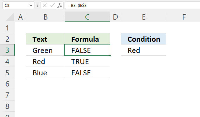
| Cells equal to «Red» | «red» |
| Cells not equal to «Red» | «<>red» |
| Cells that are blank «» | «» |
| Cells that are not blank | «<>» |
| Cells that begin with «X» | «x*» |
| Cells less than A1 | «<«&A1 |
| Cells less than today | «<«&TODAY() |
Notice the last two examples involve concatenation with the ampersand (&) character. Any time you are using a value from another cell, or using the result of a formula in criteria with a logical operator like «<«, you will need to concatenate. This is because Excel needs to evaluate cell references and formulas first to get a value, before that value can be joined to an operator.
Basic example
In the worksheet shown above, the following formulas are used in cells G5, G6, and G7:
=COUNTIF(D5:D12,">100") // count sales over 100
=COUNTIF(B5:B12,"jim") // count name = "jim"
=COUNTIF(C5:C12,"ca") // count state = "ca"
Notice COUNTIF is not case-sensitive, «CA» and «ca» are treated the same.
Double quotes («») in criteria
In general, text values need to be enclosed in double quotes («»), and numbers do not. However, when a logical operator is included with a number, the number and operator must be enclosed in quotes, as seen in the second example below:
=COUNTIF(A1:A10,100) // count cells equal to 100
=COUNTIF(A1:A10,">32") // count cells greater than 32
=COUNTIF(A1:A10,"jim") // count cells equal to "jim"
Value from another cell
A value from another cell can be included in criteria using concatenation. In the example below, COUNTIF will return the count of values in A1:A10 that are less than the value in cell B1. Notice the less than operator (which is text) is enclosed in quotes.
=COUNTIF(A1:A10,"<"&B1) // count cells less than B1
Not equal to
To construct «not equal to» criteria, use the «<>» operator surrounded by double quotes («»). For example, the formula below will count cells not equal to «red» in the range A1:A10:
=COUNTIF(A1:A10,"<>red") // not "red"
Blank cells
COUNTIF can count cells that are blank or not blank. The formulas below count blank and not blank cells in the range A1:A10:
=COUNTIF(A1:A10,"<>") // not blank
=COUNTIF(A1:A10,"") // blank
Note: be aware that COUNTIF treats formulas that return an empty string («») as not blank. See this example for some workarounds to this problem.
Dates
The easiest way to use COUNTIF with dates is to refer to a valid date in another cell with a cell reference. For example, to count cells in A1:A10 that contain a date greater than the date in B1, you can use a formula like this:
=COUNTIF(A1:A10, ">"&B1) // count dates greater than A1
Notice we must concatenate an operator to the date in B1. To use more advanced date criteria (i.e. all dates in a given month, or all dates between two dates) you’ll want to switch to the COUNTIFS function, which can handle multiple criteria.
The safest way to hardcode a date into COUNTIF is to use the DATE function. This ensures Excel will understand the date. To count cells in A1:A10 that contain a date less than April 1, 2020, you can use a formula like this
=COUNTIF(A1:A10,"<"&DATE(2020,4,1)) // dates less than 1-Apr-2020
Wildcards
The wildcard characters question mark (?), asterisk(*), or tilde (~) can be used in criteria. A question mark (?) matches any one character and an asterisk (*) matches zero or more characters of any kind. For example, to count cells in A1:A5 that contain the text «apple» anywhere, you can use a formula like this:
=COUNTIF(A1:A5,"*apple*") // cells that contain "apple"
To count cells in A1:A5 that contain any 3 text characters, you can use:
=COUNTIF(A1:A5,"???") // cells that contain any 3 characters
The tilde (~) is an escape character to match literal wildcards. For example, to count a literal question mark (?), asterisk(*), or tilde (~), add a tilde in front of the wildcard (i.e. ~?, ~*, ~~).
OR logic
The COUNTIF function is designed to apply just one condition. However, to count cells that contain «this OR that», you can use an array constant and the SUM function like this:
=SUM(COUNTIF(range,{"red","blue"})) // red or blue
The formula above will count cells in range that contain «red» or «blue». Essentially, COUNTIF returns two counts in an array (one for «red» and one for «blue») and the SUM function returns the sum. For more information, see this example.
Limitations
The COUNTIF function has some limitations you should be aware of:
- COUNTIF only supports a single condition. If you need to count cells using multiple criteria, use the COUNTIFS function.
- COUNTIF requires an actual range for the range argument; you can’t provide an array. This means you can’t alter values in range before applying criteria.
- COUNTIF is not case-sensitive. Use the EXACT function for case-sensitive counts.
- COUNTIFS has other quirks explained in this article.
The most common way to work around the limitations above is to use the SUMPRODUCT function. In the current version of Excel, another option is to use the newer BYROW and BYCOL functions.
Notes
- Text strings in criteria must be enclosed in double quotes («»), i.e. «apple», «>32», «app*»
- Cell references in criteria are not enclosed in quotes, i.e. «<«&A1
- The wildcard characters ? and * can be used in criteria. A question mark matches any one character and an asterisk matches any sequence of characters (zero or more).
- To match a literal question mark(?) or asterisk (*), use a tilde (~) like (~?, ~*).
- COUNTIF requires a range, you can’t substitute an array.
- COUNTIF returns incorrect results when used to match strings longer than 255 characters.
- COUNTIF will return a #VALUE error when referencing another workbook that is closed.
Excel has many functions where a user needs to specify a single or multiple criteria to get the result. For example, if you want to count cells based on multiple criteria, you can use the COUNTIF or COUNTIFS functions in Excel.
This tutorial covers various ways of using a single or multiple criteria in COUNTIF and COUNTIFS function in Excel.
While I will primarily be focussing on COUNTIF and COUNTIFS functions in this tutorial, all these examples can also be used in other Excel functions that take multiple criteria as inputs (such as SUMIF, SUMIFS, AVERAGEIF, and AVERAGEIFS).
An Introduction to Excel COUNTIF and COUNTIFS Functions
Let’s first get a grip on using COUNTIF and COUNTIFS functions in Excel.
Excel COUNTIF Function (takes Single Criteria)
Excel COUNTIF function is best suited for situations when you want to count cells based on a single criterion. If you want to count based on multiple criteria, use COUNTIFS function.
Syntax
=COUNTIF(range, criteria)
Input Arguments
- range – the range of cells which you want to count.
- criteria – the criteria that must be evaluated against the range of cells for a cell to be counted.
Excel COUNTIFS Function (takes Multiple Criteria)
Excel COUNTIFS function is best suited for situations when you want to count cells based on multiple criteria.
Syntax
=COUNTIFS(criteria_range1, criteria1, [criteria_range2, criteria2]…)
Input Arguments
- criteria_range1 – The range of cells for which you want to evaluate against criteria1.
- criteria1 – the criteria which you want to evaluate for criteria_range1 to determine which cells to count.
- [criteria_range2] – The range of cells for which you want to evaluate against criteria2.
- [criteria2] – the criteria which you want to evaluate for criteria_range2 to determine which cells to count.
Now let’s have a look at some examples of using multiple criteria in COUNTIF functions in Excel.
Using NUMBER Criteria in Excel COUNTIF Functions
#1 Count Cells when Criteria is EQUAL to a Value
To get the count of cells where the criteria argument is equal to a specified value, you can either directly enter the criteria or use the cell reference that contains the criteria.
Below is an example where we count the cells that contain the number 9 (which means that the criteria argument is equal to 9). Here is the formula:
=COUNTIF($B$2:$B$11,D3)

In the above example (in the pic), the criteria is in cell D3. You can also enter the criteria directly into the formula. For example, you can also use:
=COUNTIF($B$2:$B$11,9)
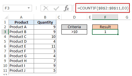
#2 Count Cells when Criteria is GREATER THAN a Value
To get the count of cells with a value greater than a specified value, we use the greater than operator (“>”). We could either use it directly in the formula or use a cell reference that has the criteria.
Whenever we use an operator in criteria in Excel, we need to put it within double quotes. For example, if the criteria is greater than 10, then we need to enter “>10” as the criteria (see pic below):
Here is the formula:
=COUNTIF($B$2:$B$11,”>10″)

You can also have the criteria in a cell and use the cell reference as the criteria. In this case, you need NOT put the criteria in double quotes:
=COUNTIF($B$2:$B$11,D3)
There could also be a case when you want the criteria to be in a cell, but don’t want it with the operator. For example, you may want the cell D3 to have the number 10 and not >10.
In that case, you need to create a criteria argument which is a combination of operator and cell reference (see pic below):
=COUNTIF($B$2:$B$11,”>”&D3)
 NOTE: When you combine an operator and a cell reference, the operator is always in double quotes. The operator and cell reference are joined by an ampersand (&).
#3 Count Cells when Criteria is LESS THAN a Value
To get the count of cells with a value less than a specified value, we use the less than operator (“<“). We could either use it directly in the formula or use a cell reference that has the criteria.
Whenever we use an operator in criteria in Excel, we need to put it within double quotes. For example, if the criterion is that the number should be less than 5, then we need to enter “<5” as the criteria (see pic below):
=COUNTIF($B$2:$B$11,”<5″)

You can also have the criteria in a cell and use the cell reference as the criteria. In this case, you need NOT put the criteria in double quotes (see pic below):
=COUNTIF($B$2:$B$11,D3)

Also, there could be a case when you want the criteria to be in a cell, but don’t want it with the operator. For example, you may want the cell D3 to have the number 5 and not <5.
In that case, you need to create a criteria argument which is a combination of operator and cell reference:
=COUNTIF($B$2:$B$11,”<“&D3)

NOTE: When you combine an operator and a cell reference, the operator is always in double quotes. The operator and cell reference are joined by an ampersand (&).
#4 Count Cells with Multiple Criteria – Between Two Values
To get a count of values between two values, we need to use multiple criteria in the COUNTIF function.
Here are two methods of doing this:
METHOD 1: Using COUNTIFS function
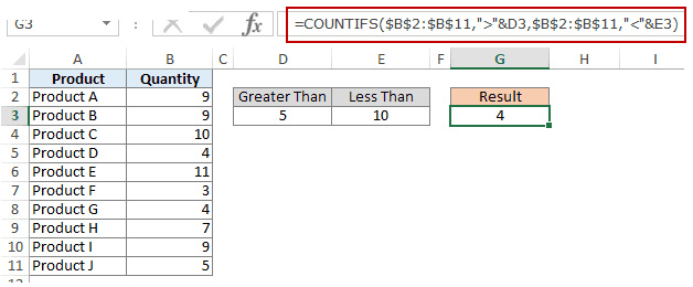
COUNTIFS function can handle multiple criteria as arguments and counts the cells only when all the criteria are TRUE. To count cells with values between two specified values (say 5 and 10), we can use the following COUNTIFS function:
=COUNTIFS($B$2:$B$11,”>5″,$B$2:$B$11,”<10″)

NOTE: The above formula does not count cells that contain 5 or 10. If you want to include these cells, use greater than equal to (>=) and less than equal to (<=) operators. Here is the formula:
=COUNTIFS($B$2:$B$11,”>=5″,$B$2:$B$11,”<=10″)
You can also have these criteria in cells and use the cell reference as the criteria. In this case, you need NOT put the criteria in double quotes (see pic below):

You can also use a combination of cells references and operators (where the operator is entered directly in the formula). When you combine an operator and a cell reference, the operator is always in double quotes. The operator and cell reference are joined by an ampersand (&).
METHOD 2: Using two COUNTIF functions
If you have multiple criteria, you can either use COUNTIFS or create a combination of COUNTIF functions. The formula below would also do the same thing:
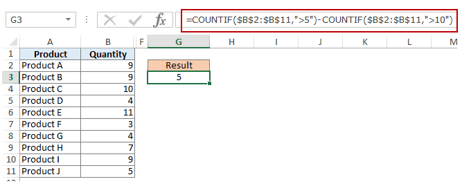
=COUNTIF($B$2:$B$11,”>5″)-COUNTIF($B$2:$B$11,”>10″)
In the above formula, we first find the number of cells that have a value greater than 5 and we subtract the count of cells with a value greater than 10. This would give us the result as 5 (which is the number of cells that have values more than 5 and less than equal to 10).
If you want the formula to include both 5 and 10, use the following formula instead:
=COUNTIF($B$2:$B$11,”>=5″)-COUNTIF($B$2:$B$11,”>10″)
If you want the formula to exclude both ‘5’ and ’10’ from the counting, use the following formula:
=COUNTIF($B$2:$B$11,”>=5″)-COUNTIF($B$2:$B$11,”>10″)-COUNTIF($B$2:$B$11,10)
You can have these criteria in cells and use the cells references, or you can use a combination of operators and cells references.
Using TEXT Criteria in Excel Functions
#1 Count Cells when Criteria is EQUAL to a Specified text
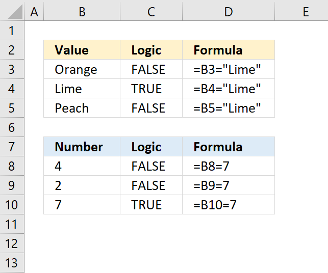
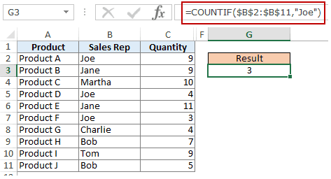
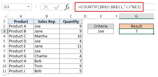
To count cells that contain an exact match of the specified text, we can simply use that text as the criteria. For example, in the dataset (shown below in the pic), if I want to count all the cells with the name Joe in it, I can use the below formula:
=COUNTIF($B$2:$B$11,”Joe”)
Since this is a text string, I need to put the text criteria in double quotes.
You can also have the criteria in a cell and then use that cell reference (as shown below):
=COUNTIF($B$2:$B$11,E3)

NOTE: You can get wrong results if there are leading/trailing spaces in the criteria or criteria range. Make sure you clean the data before using these formulas.
#2 Count Cells when Criteria is NOT EQUAL to a Specified text
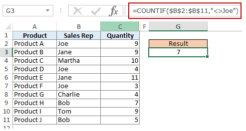
Similar to what we saw in the above example, you can also count cells that do not contain a specified text. To do this, we need to use the not equal to operator (<>).
Suppose you want to count all the cells that do not contain the name JOE, here is the formula that will do it:
=COUNTIF($B$2:$B$11,”<>Joe”)
You can also have the criteria in a cell and use the cell reference as the criteria. In this case, you need NOT put the criteria in double quotes (see pic below):
=COUNTIF($B$2:$B$11,E3)
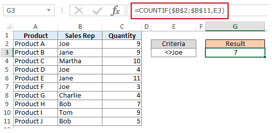
There could also be a case when you want the criteria to be in a cell but don’t want it with the operator. For example, you may want the cell D3 to have the name Joe and not <>Joe.
In that case, you need to create a criteria argument which is a combination of operator and cell reference (see pic below):
=COUNTIF($B$2:$B$11,”<>”&E3)
When you combine an operator and a cell reference, the operator is always in double quotes. The operator and cell reference are joined by an ampersand (&).
Using DATE Criteria in Excel COUNTIF and COUNTIFS Functions
Excel store date and time as numbers. So we can use it the same way we use numbers.
#1 Count Cells when Criteria is EQUAL to a Specified Date
To get the count of cells that contain the specified date, we would use the equal to operator (=) along with the date.
To use the date, I recommend using the DATE function, as it gets rid of any possibility of error in the date value. So, for example, if I want to use the date September 1, 2015, I can use the DATE function as shown below:
=DATE(2015,9,1)
This formula would return the same date despite regional differences. For example, 01-09-2015 would be September 1, 2015 according to the US date syntax and January 09, 2015 according to the UK date syntax. However, this formula would always return September 1, 2105.
Here is the formula to count the number of cells that contain the date 02-09-2015:
=COUNTIF($A$2:$A$11,DATE(2015,9,2))

#2 Count Cells when Criteria is BEFORE or AFTER to a Specified Date
To count cells that contain date before or after a specified date, we can use the less than/greater than operators.
For example, if I want to count all the cells that contain a date that is after September 02, 2015, I can use the formula:
=COUNTIF($A$2:$A$11,”>”&DATE(2015,9,2))

Similarly, you can also count the number of cells before a specified date. If you want to include a date in the counting, use and ‘equal to’ operator along with ‘greater than/less than’ operator.
You can also use a cell reference that contains a date. In this case, you need to combine the operator (within double quotes) with the date using an ampersand (&).
See example below:
=COUNTIF($A$2:$A$11,”>”&F3)

#3 Count Cells with Multiple Criteria – Between Two Dates
To get a count of values between two values, we need to use multiple criteria in the COUNTIF function.
We can do this using two methods – One single COUNTIFS function or two COUNTIF functions.
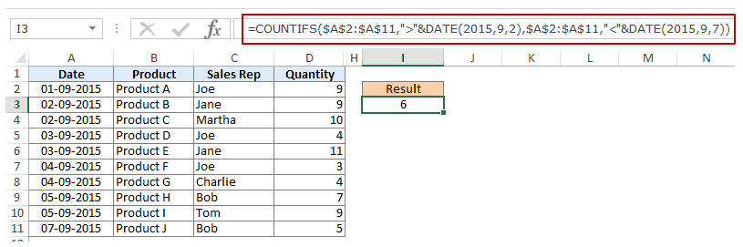
METHOD 1: Using COUNTIFS function
COUNTIFS function can take multiple criteria as the arguments and counts the cells only when all the criteria are TRUE. To count cells with values between two specified dates (say September 2 and September 7), we can use the following COUNTIFS function:
=COUNTIFS($A$2:$A$11,”>”&DATE(2015,9,2),$A$2:$A$11,”<“&DATE(2015,9,7))
The above formula does not count cells that contain the specified dates. If you want to include these dates as well, use greater than equal to (>=) and less than equal to (<=) operators. Here is the formula:
=COUNTIFS($A$2:$A$11,”>=”&DATE(2015,9,2),$A$2:$A$11,”<=”&DATE(2015,9,7))
You can also have the dates in a cell and use the cell reference as the criteria. In this case, you can not have the operator with the date in the cells. You need to manually add operators in the formula (in double quotes) and add cell reference using an ampersand (&). See the pic below:
=COUNTIFS($A$2:$A$11,”>”&F3,$A$2:$A$11,”<“&G3)

METHOD 2: Using COUNTIF functions
If you have multiple criteria, you can either use one COUNTIFS function or create a combination of two COUNTIF functions. The formula below would also do the trick:
=COUNTIF($A$2:$A$11,”>”&DATE(2015,9,2))-COUNTIF($A$2:$A$11,”>”&DATE(2015,9,7))
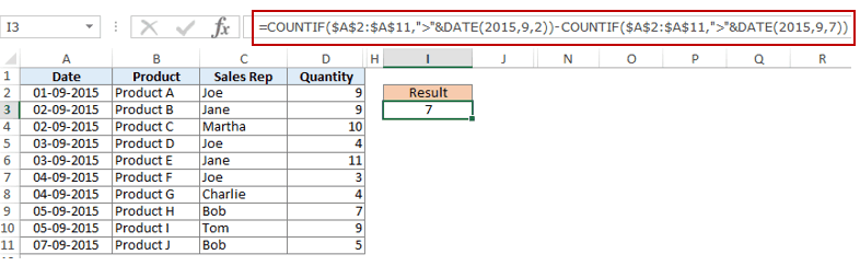
In the above formula, we first find the number of cells that have a date after September 2 and we subtract the count of cells with dates after September 7. This would give us the result as 7 (which is the number of cells that have dates after September 2 and on or before September 7).
If you don’t want the formula to count both September 2 and September 7, use the following formula instead:
=COUNTIF($A$2:$A$11,”>=”&DATE(2015,9,2))-COUNTIF($A$2:$A$11,”>”&DATE(2015,9,7))

If you want to exclude both the dates from counting, use the following formula:
=COUNTIF($A$2:$A$11,”>”&DATE(2015,9,2))-COUNTIF($A$2:$A$11,”>”&DATE(2015,9,7)-COUNTIF($A$2:$A$11,DATE(2015,9,7)))
Also, you can have the criteria dates in cells and use the cells references (along with operators in double quotes joined using ampersand).
Using WILDCARD CHARACTERS in Criteria in COUNTIF & COUNTIFS Functions
There are three wildcard characters in Excel:
- * (asterisk) – It represents any number of characters. For example, ex* could mean excel, excels, example, expert, etc.
- ? (question mark) – It represents one single character. For example, Tr?mp could mean Trump or Tramp.
- ~ (tilde) – It is used to identify a wildcard character (~, *, ?) in the text.
You can use COUNTIF function with wildcard characters to count cells when other inbuilt count function fails. For example, suppose you have a data set as shown below:
Now let’s take various examples:
#1 Count Cells that contain Text
To count cells with text in it, we can use the wildcard character * (asterisk). Since asterisk represents any number of characters, it would count all cells that have any text in it. Here is the formula:
=COUNTIFS($C$2:$C$11,”*”)
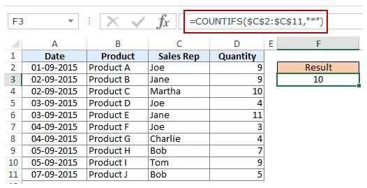
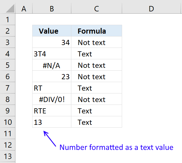
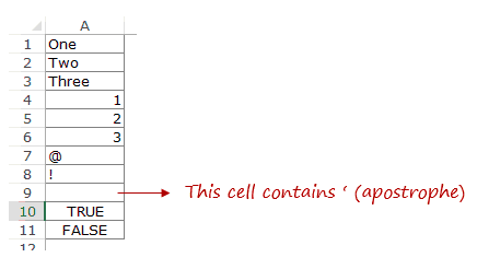
Note: The formula above ignores cells that contain numbers, blank cells, and logical values, but would count the cells contain an apostrophe (and hence appear blank) or cells that contain empty string (=””) which may have been returned as a part of a formula.
Here is a detailed tutorial on handling cases where there is an empty string or apostrophe.
Here is a detailed tutorial on handling cases where there are empty strings or apostrophes.
Below is a video that explains different scenarios of counting cells with text in it.
#2 Count Non-blank Cells
If you are thinking of using COUNTA function, think again.
Try it and it might fail you. COUNTA will also count a cell that contains an empty string (often returned by formulas as =”” or when people enter only an apostrophe in a cell). Cells that contain empty strings look blank but are not, and thus counted by the COUNTA function.
COUNTA will also count a cell that contains an empty string (often returned by formulas as =”” or when people enter only an apostrophe in a cell). Cells that contain empty strings look blank but are not, and thus counted by the COUNTA function.
So if you use the formula =COUNTA(A1:A11), it returns 11, while it should return 10.
Here is the fix:
=COUNTIF($A$1:$A$11,”?*”)+COUNT($A$1:$A$11)+SUMPRODUCT(–ISLOGICAL($A$1:$A$11))
Let’s understand this formula by breaking it down:
#3 Count Cells that contain specific text
Let’s say we want to count all the cells where the sales rep name begins with J. This can easily be achieved by using a wildcard character in COUNTIF function. Here is the formula:
=COUNTIFS($C$2:$C$11,”J*”)

The criteria J* specifies that the text in a cell should begin with J and can contain any number of characters.
If you want to count cells that contain the alphabet anywhere in the text, flank it with an asterisk on both sides. For example, if you want to count cells that contain the alphabet “a” in it, use *a* as the criteria.
This article is unusually long compared to my other articles. Hope you have enjoyed it. Let me know your thoughts by leaving a comment.
You May Also Find the following Excel tutorials useful:
- Count the number of words in Excel.
- Count Cells Based on Background Color in Excel.
- How to Sum a Column in Excel (5 Really Easy Ways)