
-
Select the cell where you want the result to appear.
-
On the Formulas tab, click More Functions, point to Statistical, and then click one of the following functions:
-
COUNTA: To count cells that are not empty
-
COUNT: To count cells that contain numbers.
-
COUNTBLANK: To count cells that are blank.
-
COUNTIF: To count cells that meets a specified criteria.
Tip: To enter more than one criterion, use the COUNTIFS function instead.
-
-
Select the range of cells that you want, and then press RETURN.
-
Select the cell where you want the result to appear.
-
On the Formulas tab, click Insert, point to Statistical, and then click one of the following functions:
-
COUNTA: To count cells that are not empty
-
COUNT: To count cells that contain numbers.
-
COUNTBLANK: To count cells that are blank.
-
COUNTIF: To count cells that meets a specified criteria.
Tip: To enter more than one criterion, use the COUNTIFS function instead.
-
-
Select the range of cells that you want, and then press RETURN.
Counting is an integral part of data analysis, whether you are tallying the head count of a department in your organization or the number of units that were sold quarter-by-quarter. Excel provides multiple techniques that you can use to count cells, rows, or columns of data. To help you make the best choice, this article provides a comprehensive summary of methods, a downloadable workbook with interactive examples, and links to related topics for further understanding.
Download our examples
You can download an example workbook that gives examples to supplement the information in this article. Most sections in this article will refer to the appropriate worksheet within the example workbook that provides examples and more information.
Download examples to count values in a spreadsheet
In this article
-
Simple counting
-
Use AutoSum
-
Add a Subtotal row
-
Count cells in a list or Excel table column by using the SUBTOTAL function
-
-
Counting based on one or more conditions
-
Video: Use the COUNT, COUNTIF, and COUNTA functions
-
Count cells in a range by using the COUNT function
-
Count cells in a range based on a single condition by using the COUNTIF function
-
Count cells in a column based on single or multiple conditions by using the DCOUNT function
-
Count cells in a range based on multiple conditions by using the COUNTIFS function
-
Count based on criteria by using the COUNT and IF functions together
-
Count how often multiple text or number values occur by using the SUM and IF functions together
-
Count cells in a column or row in a PivotTable
-
-
Counting when your data contains blank values
-
Count nonblank cells in a range by using the COUNTA function
-
Count nonblank cells in a list with specific conditions by using the DCOUNTA function
-
Count blank cells in a contiguous range by using the COUNTBLANK function
-
Count blank cells in a non-contiguous range by using a combination of SUM and IF functions
-
-
Counting unique occurrences of values
-
Count the number of unique values in a list column by using Advanced Filter
-
Count the number of unique values in a range that meet one or more conditions by using IF, SUM, FREQUENCY, MATCH, and LEN functions
-
-
Special cases (count all cells, count words)
-
Count the total number of cells in a range by using ROWS and COLUMNS functions
-
Count words in a range by using a combination of SUM, IF, LEN, TRIM, and SUBSTITUTE functions
-
-
Displaying calculations and counts on the status bar
Simple counting
You can count the number of values in a range or table by using a simple formula, clicking a button, or by using a worksheet function.
Excel can also display the count of the number of selected cells on the Excel status bar. See the video demo that follows for a quick look at using the status bar. Also, see the section Displaying calculations and counts on the status bar for more information. You can refer to the values shown on the status bar when you want a quick glance at your data and don’t have time to enter formulas.
Video: Count cells by using the Excel status bar
Watch the following video to learn how to view count on the status bar.

Use AutoSum
Use AutoSum by selecting a range of cells that contains at least one numeric value. Then on the Formulas tab, click AutoSum > Count Numbers.

Excel returns the count of the numeric values in the range in a cell adjacent to the range you selected. Generally, this result is displayed in a cell to the right for a horizontal range or in a cell below for a vertical range.
Top of Page
Add a Subtotal row
You can add a subtotal row to your Excel data. Click anywhere inside your data, and then click Data > Subtotal.
Note: The Subtotal option will only work on normal Excel data, and not Excel tables, PivotTables, or PivotCharts.

Also, refer to the following articles:
-
Outline (group) data in a worksheet
-
Insert subtotals in a list of data in a worksheet
Top of Page
Count cells in a list or Excel table column by using the SUBTOTAL function
Use the SUBTOTAL function to count the number of values in an Excel table or range of cells. If the table or range contains hidden cells, you can use SUBTOTAL to include or exclude those hidden cells, and this is the biggest difference between SUM and SUBTOTAL functions.
The SUBTOTAL syntax goes like this:
SUBTOTAL(function_num,ref1,[ref2],…)

To include hidden values in your range, you should set the function_num argument to 2.
To exclude hidden values in your range, set the function_num argument to 102.
Top of Page
Counting based on one or more conditions
You can count the number of cells in a range that meet conditions (also known as criteria) that you specify by using a number of worksheet functions.
Video: Use the COUNT, COUNTIF, and COUNTA functions
Watch the following video to see how to use the COUNT function and how to use the COUNTIF and COUNTA functions to count only the cells that meet conditions you specify.
Top of Page
Count cells in a range by using the COUNT function
Use the COUNT function in a formula to count the number of numeric values in a range.

In the above example, A2, A3, and A6 are the only cells that contains numeric values in the range, hence the output is 3.
Note: A7 is a time value, but it contains text (a.m.), hence COUNT does not consider it a numerical value. If you were to remove a.m. from the cell, COUNT will consider A7 as a numerical value, and change the output to 4.
Top of Page
Count cells in a range based on a single condition by using the COUNTIF function
Use the COUNTIF function function to count how many times a particular value appears in a range of cells.

Top of Page
Count cells in a column based on single or multiple conditions by using the DCOUNT function
DCOUNT function counts the cells that contain numbers in a field (column) of records in a list or database that match conditions that you specify.
In the following example, you want to find the count of the months including or later than March 2016 that had more than 400 units sold. The first table in the worksheet, from A1 to B7, contains the sales data.

DCOUNT uses conditions to determine where the values should be returned from. Conditions are typically entered in cells in the worksheet itself, and you then refer to these cells in the criteria argument. In this example, cells A10 and B10 contain two conditions—one that specifies that the return value must be greater than 400, and the other that specifies that the ending month should be equal to or greater than March 31st, 2016.
You should use the following syntax:
=DCOUNT(A1:B7,»Month ending»,A9:B10)
DCOUNT checks the data in the range A1 through B7, applies the conditions specified in A10 and B10, and returns 2, the total number of rows that satisfy both conditions (rows 5 and 7).
Top of Page
Count cells in a range based on multiple conditions by using the COUNTIFS function
The COUNTIFS function is similar to the COUNTIF function with one important exception: COUNTIFS lets you apply criteria to cells across multiple ranges and counts the number of times all criteria are met. You can use up to 127 range/criteria pairs with COUNTIFS.
The syntax for COUNTIFS is:
COUNTIFS(criteria_range1, criteria1, [criteria_range2, criteria2],…)
See the following example:

Top of Page
Count based on criteria by using the COUNT and IF functions together
Let’s say you need to determine how many salespeople sold a particular item in a certain region or you want to know how many sales over a certain value were made by a particular salesperson. You can use the IF and COUNT functions together; that is, you first use the IF function to test a condition and then, only if the result of the IF function is True, you use the COUNT function to count cells.
Notes:
-
The formulas in this example must be entered as array formulas. If you have opened this workbook in Excel for Windows or Excel 2016 for Mac and want to change the formula or create a similar formula, press F2, and then press Ctrl+Shift+Enter to make the formula return the results you expect. In earlier versions of Excel for Mac, use
 +Shift+Enter.
 -
For the example formulas to work, the second argument for the IF function must be a number.

Top of Page
Count how often multiple text or number values occur by using the SUM and IF functions together
In the examples that follow, we use the IF and SUM functions together. The IF function first tests the values in some cells and then, if the result of the test is True, SUM totals those values that pass the test.
Example 1

The above function says if C2:C7 contains the values Buchanan and Dodsworth, then the SUM function should display the sum of records where the condition is met. The formula finds three records for Buchanan and one for Dodsworth in the given range, and displays 4.
Example 2

The above function says if D2:D7 contains values lesser than $9000 or greater than $19,000, then SUM should display the sum of all those records where the condition is met. The formula finds two records D3 and D5 with values lesser than $9000, and then D4 and D6 with values greater than $19,000, and displays 4.
Example 3

The above function says if D2:D7 has invoices for Buchanan for less than $9000, then SUM should display the sum of records where the condition is met. The formula finds that C6 meets the condition, and displays 1.
Important: The formulas in this example must be entered as array formulas. That means you press F2 and then press Ctrl+Shift+Enter. In earlier versions of Excel for Mac use  +Shift+Enter.
See the following Knowledge Base articles for additional tips:
-
XL: Using SUM(IF()) As an Array Function Instead of COUNTIF() with AND
-
XL: How to Count the Occurrences of a Number or Text in a Range
Top of Page
Count cells in a column or row in a PivotTable
A PivotTable summarizes your data and helps you analyze and drill down into your data by letting you choose the categories on which you want to view your data.
You can quickly create a PivotTable by selecting a cell in a range of data or Excel table and then, on the Insert tab, in the Tables group, clicking PivotTable.

Let’s look at a sample scenario of a Sales spreadsheet, where you can count how many sales values are there for Golf and Tennis for specific quarters.
Note: For an interactive experience, you can run these steps on the sample data provided in the PivotTable sheet in the downloadable workbook.
-
Enter the following data in an Excel spreadsheet.
-
Select A2:C8
-
Click Insert > PivotTable.
-
In the Create PivotTable dialog box, click Select a table or range, then click New Worksheet, and then click OK.
An empty PivotTable is created in a new sheet.
-
In the PivotTable Fields pane, do the following:
-
Drag Sport to the Rows area.
-
Drag Quarter to the Columns area.
-
Drag Sales to the Values area.
-
Repeat step c.
The field name displays as SumofSales2 in both the PivotTable and the Values area.
At this point, the PivotTable Fields pane looks like this:
-
In the Values area, click the dropdown next to SumofSales2 and select Value Field Settings.
-
In the Value Field Settings dialog box, do the following:
-
In the Summarize value field by section, select Count.
-
In the Custom Name field, modify the name to Count.
-
Click OK.
-
The PivotTable displays the count of records for Golf and Tennis in Quarter 3 and Quarter 4, along with the sales figures.
-


Top of Page
Counting when your data contains blank values
You can count cells that either contain data or are blank by using worksheet functions.
Count nonblank cells in a range by using the COUNTA function
Use the COUNTA function function to count only cells in a range that contain values.
When you count cells, sometimes you want to ignore any blank cells because only cells with values are meaningful to you. For example, you want to count the total number of salespeople who made a sale (column D).

COUNTA ignores the blank values in D3, D4, D8, and D11, and counts only the cells containing values in column D. The function finds six cells in column D containing values and displays 6 as the output.
Top of Page
Count nonblank cells in a list with specific conditions by using the DCOUNTA function
Use the DCOUNTA function to count nonblank cells in a column of records in a list or database that match conditions that you specify.
The following example uses the DCOUNTA function to count the number of records in the database that is contained in the range A1:B7 that meet the conditions specified in the criteria range A9:B10. Those conditions are that the Product ID value must be greater than or equal to 2000 and the Ratings value must be greater than or equal to 50.

DCOUNTA finds two rows that meet the conditions- rows 2 and 4, and displays the value 2 as the output.
Top of Page
Count blank cells in a contiguous range by using the COUNTBLANK function
Use the COUNTBLANK function function to return the number of blank cells in a contiguous range (cells are contiguous if they are all connected in an unbroken sequence). If a cell contains a formula that returns empty text («»), that cell is counted.
When you count cells, there may be times when you want to include blank cells because they are meaningful to you. In the following example of a grocery sales spreadsheet. suppose you want to find out how many cells don’t have the sales figures mentioned.

Note: The COUNTBLANK worksheet function provides the most convenient method for determining the number of blank cells in a range, but it doesn’t work very well when the cells of interest are in a closed workbook or when they do not form a contiguous range. The Knowledge Base article XL: When to Use SUM(IF()) instead of CountBlank() shows you how to use a SUM(IF()) array formula in those cases.
Top of Page
Count blank cells in a non-contiguous range by using a combination of SUM and IF functions
Use a combination of the SUM function and the IF function. In general, you do this by using the IF function in an array formula to determine whether each referenced cell contains a value, and then summing the number of FALSE values returned by the formula.
See a few examples of SUM and IF function combinations in an earlier section Count how often multiple text or number values occur by using the SUM and IF functions together in this topic.
Top of Page
Counting unique occurrences of values
You can count unique values in a range by using a PivotTable, COUNTIF function, SUM and IF functions together, or the Advanced Filter dialog box.
Count the number of unique values in a list column by using Advanced Filter
Use the Advanced Filter dialog box to find the unique values in a column of data. You can either filter the values in place or you can extract and paste them to a new location. Then you can use the ROWS function to count the number of items in the new range.
To use Advanced Filter, click the Data tab, and in the Sort & Filter group, click Advanced.
The following figure shows how you use the Advanced Filter to copy only the unique records to a new location on the worksheet.

In the following figure, column E contains the values that were copied from the range in column D.

Notes:
-
If you filter your data in place, values are not deleted from your worksheet — one or more rows might be hidden. Click Clear in the Sort & Filter group on the Data tab to display those values again.
-
If you only want to see the number of unique values at a quick glance, select the data after you have used the Advanced Filter (either the filtered or the copied data) and then look at the status bar. The Count value on the status bar should equal the number of unique values.
For more information, see Filter by using advanced criteria
Top of Page
Count the number of unique values in a range that meet one or more conditions by using IF, SUM, FREQUENCY, MATCH, and LEN functions
Use various combinations of the IF, SUM, FREQUENCY, MATCH, and LEN functions.
For more information and examples, see the section «Count the number of unique values by using functions» in the article Count unique values among duplicates.
Top of Page
Special cases (count all cells, count words)
You can count the number of cells or the number of words in a range by using various combinations of worksheet functions.
Count the total number of cells in a range by using ROWS and COLUMNS functions
Suppose you want to determine the size of a large worksheet to decide whether to use manual or automatic calculation in your workbook. To count all the cells in a range, use a formula that multiplies the return values using the ROWS and COLUMNS functions. See the following image for an example:

Top of Page
Count words in a range by using a combination of SUM, IF, LEN, TRIM, and SUBSTITUTE functions
You can use a combination of the SUM, IF, LEN, TRIM, and SUBSTITUTE functions in an array formula. The following example shows the result of using a nested formula to find the number of words in a range of 7 cells (3 of which are empty). Some of the cells contain leading or trailing spaces — the TRIM and SUBSTITUTE functions remove these extra spaces before any counting occurs. See the following example:

Now, for the above formula to work correctly, you have to make this an array formula, otherwise the formula returns the #VALUE! error. To do that, click on the cell that has the formula, and then in the Formula bar, press Ctrl + Shift + Enter. Excel adds a curly bracket at the beginning and the end of the formula, thus making it an array formula.
For more information on array formulas, see Overview of formulas in Excel and Create an array formula.
Top of Page
Displaying calculations and counts on the status bar
When one or more cells are selected, information about the data in those cells is displayed on the Excel status bar. For example, if four cells on your worksheet are selected, and they contain the values 2, 3, a text string (such as «cloud»), and 4, all of the following values can be displayed on the status bar at the same time: Average, Count, Numerical Count, Min, Max, and Sum. Right-click the status bar to show or hide any or all of these values. These values are shown in the illustration that follows.

Top of Page
Need more help?
You can always ask an expert in the Excel Tech Community or get support in the Answers community.
What Is COUNT In Excel?
The COUNT function in Excel counts the number of cells containing numerical values within the given range. It always returns an integer value.
The COUNT in Excel is an inbuilt statistical function, so we can insert the formula from the “Function Library” or enter it directly in the worksheet.
For example, to count a range of cells that contain a date before April 1, 2021, the formula used is “=COUNT(“Cell Range”, “<”&DATE (2021,4,1))”. The date is entered by using the DATE functionThe date function in excel is a date and time function representing the number provided as arguments in a date and time code. The result displayed is in date format, but the arguments are supplied as integers.read more.
Table of contents
- What Is COUNT In Excel?
- Syntax Of COUNT Excel Formula
- How To Use COUNT Function In Excel?
- Examples
- The Characteristics Of The COUNT Function
- Important Things To Note
- Frequently Asked Questions (FAQs)
- COUNT Function In Excel Video
- Download Template
- Recommended Articles
- In a given dataset, the COUNT function in Excel returns the count of the numeric values.
- It counts only the numbers and not the logical values, empty cells, text, or error values when the argument seems to be an array or reference.
- The usage of the COUNT and VBA (VBA Excel COUNT) functions are the same in Excel.
- The COUNTA function is a further extension of the COUNT function. It counts logical values, text, or error values. The COUNTIF function (another extension of the COUNT function) counts the numbers that meet a specified criterion.
Syntax Of COUNT Excel Formula
The syntax of the COUNT Excel formula is,
The arguments of the COUNT Excel formula are,
- value1, [value2], …, [value n]: It is a mandatory argument. It can range up to 255 values. The value can be a cell referenceCell reference in excel is referring the other cells to a cell to use its values or properties. For instance, if we have data in cell A2 and want to use that in cell A1, use =A2 in cell A1, and this will copy the A2 value in A1.read more or a range of values. It is a collection of worksheet cells containing a variety of data, out of which only the cells containing numbers are counted.
How To Use COUNT Function In Excel?
We can use the COUNT Excel function in 2 ways, namely:
- Access from the Excel ribbon.
- Enter in the worksheet manually.
Method #1 – Access from the Excel ribbon
Choose an empty cell for the result → select the “Formulas” tab → go to the “Function Library” group → click the “More Functions” option drop-down → click the “Statistical” option right arrow → select the “COUNT” function, as shown below.

The “Function Arguments” windowappears. Enter the arguments in the “Value1”, “Value2”, etc. fields, and click “OK”, as shown below.

Method #2 – Enter in the worksheet manually
- Select an empty cell for the output.
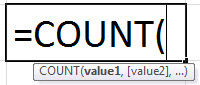
- Type =COUNT( in the selected cell. [Alternatively, type =C or =COU and double-click the COUNT function from the list of suggestions shown by Excel.
- Enter the argument as cell value or cell reference and close the brackets.
- Press the “Enter” key.
Basic Example – Count Numbers in the Given Range
Let us look at an example to apply the COUNT function to Count Numbers in the Given Range. (shown in the table below).
Select cell B10, enter the formula =COUNT(B3:B8), and press “Enter”.
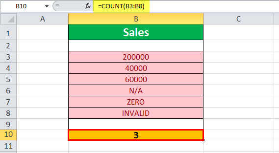
The output is shown above. The range B3:B8 contains only three numeric values. Hence, the COUNT function returns 3.
Examples
We will consider some scenarios using COUNT Function in Excel examples. Each example covers a different case, implemented using the COUNT function.
Example #1 – Count Non-empty Cells
Let us apply the COUNTA functionThe COUNTA function is an inbuilt statistical excel function that counts the number of non-blank cells (not empty) in a cell range or the cell reference. For example, cells A1 and A3 contain values but, cell A2 is empty. The formula “=COUNTA(A1,A2,A3)” returns 2.
read more to the range of cells A1:A5 provided in the below table to find the count of the number of cells that are not empty.
Select cell B1, enter the formula =COUNTA(A1:A5), and press “Enter”.

The output is shown above. The COUNTA function counts the number of cells from A1 through A5 that contain some data. It returns the value as 4, as cells A1, A2, A3, and A4 are not empty, and only cell A5 is empty.
Example #2 – Count the Number of Valid Dates
Let us apply the COUNT function to count the number of valid dates to the range of cells C3:C8 (shown in the table below).
Select cell C10, enter the formula =COUNT(C3:C8), and press “Enter”.
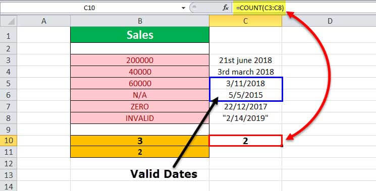
The output is shown above. The range contains dates in different formats. Out of this, only two dates are valid. Hence, the formula returns 2.
Example #3 – Multiple Parameters
Let us apply the COUNT formula to the range of excel cells C3:C7 (provided in the table below) along with another parameter that is hard-coded with a value of 5.
Select cell C11, enter the formula =COUNTA(C3:C7,5), and press “Enter”.
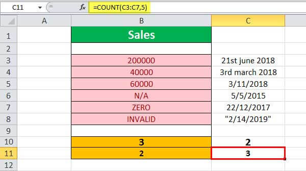
The output is shown above. The number of cells (C3 through C7) with valid numeric values or dates is 2, plus 1 for the number 5. Hence the COUNT formula returns the result as 3 (cells C5, C6, and the number 5). Note that the date in cell C7 is invalid, and so is not taken into account in the given results.
Example #4 – Invalid Numbers
Let us apply the COUNT formula to the range of values B6:B8 (shown in the table below) containing invalid numbers.
Select cell B12, enter the formula =COUNTA(B6:B8), and press “Enter”.
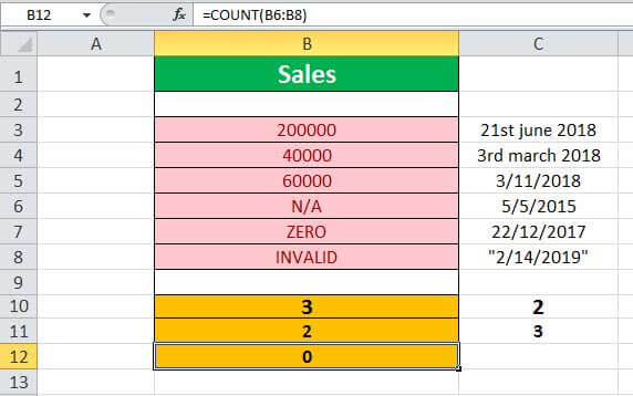
The output is shown above. The range does not have any valid number. Hence, the result returned by the formula is 0, indicated in cell B12.
Example #5 – Empty Range
Let us apply the COUNT function to the range of values in cells D3:D5, which is an empty range.
Select cell D10, enter the formula =COUNTA(D3:D5), and press “Enter”.

The output is shown above. The given range does not have any numbers, and it is empty. Hence, the result returned by the formula is 0, indicated in cell D10.
The Characteristics Of The COUNT Function
The features of the COUNT Excel function are listed as follows:
- It counts the list of parameters containing the logical values and text representations.
- It does not count the error values or text which cannot be converted into numbers.
- It counts only the numbers and not the logical values, empty cells, text, or error values when the argument seems to be an array or reference.
- A further extension to the COUNT function is the COUNTA function. It counts logical values, text, or error values.
- Another extension of the COUNT function is the COUNTIF function, which counts the numbers that meet a specified criterion.
Important Things To Note
- Since the COUNT function has other related functions such as COUNTA, COUNTIF, COUNTBLANK, etc., we must ensure we enter the right function name to avoid getting a “#NAME?” error.
- In a selected cell range, the function ignores the blank cells, non-numeric cells, etc.
Frequently Asked Questions (FAQs)
1. How to use the Excel COUNT function?
The COUNT function provides the count of cells containing numbers within the given range of cells. It also counts numeric values within the list of arguments.
The formula of the COUNT in excel is =COUNT(value 1, [value 2],……, and so on).
2. What is the COUNTIF formula?
The COUNTIF function counts cells in a range that meets a single criterion. It counts cells that contain dates, numbers, and text.
The COUNTIF formula in excel is =COUNTIF(range, condition)
Here, the range is a series of cells to count.
3. What is the difference between the COUNT and COUNTA functions in Excel?
The COUNT function is generally used to count a range of cells containing numbers or dates. It excludes blank cells. And the COUNTA function, whichstands for count all, will count the numbers, dates, text, or a range containing a mixture of all these items. It does not count blank cells.
COUNT Function In Excel Video
Download Template
This article must help understand the COUNT function in Excel with its formulas and examples. You can download the template here to use it instantly.
You can download this COUNT Formula Excel Template here – COUNT Formula Excel Template
Recommended Articles
This is a guide to the COUNT Function in Excel. Here, we count number of cells with numeric values, COUNTA, COUNTIF, examples & a downloadable template. You may also look at the below useful functions in Excel –
- Example of COUNTIF with Multiple Criteria
- INT Function in Excel (Integer)INT or integer function in excel returns the nearest integer of a given number and is used when we have many data sets and each data in a different format.read more
- AVERAGE Function in Excel
Earlier, we learned about how to count cells with numbers, count cells with text, count blank cells and count cells with specific criterias. In this article, we will learn about how to count all cells in a range in excel.
There is no individual function in excel that returns total count of cells in a given range. But this doesn’t mean we can’t count all cell in excel range. Let’s explore some formulas for counting cells in a given range.
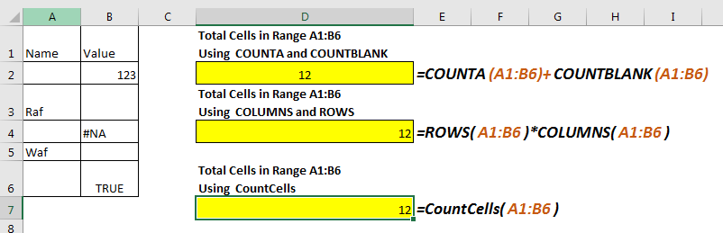
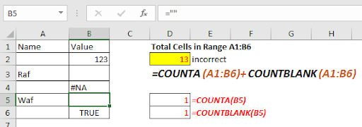
Using COUNTA and COUNTBLANK to Count Cells in a Range
*this method has problem.
As we know that t COUNTA function in excel counts any cell which is not blank. On the other hand COUNTBLANK function counts blank cell in a range. Yes, you guessed it write, we can add them to get total number of cells.
Generic Formula to Count Cells
=COUNTA(range)+COUNTBLANK(range)
Example
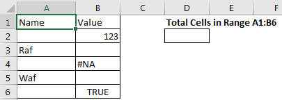
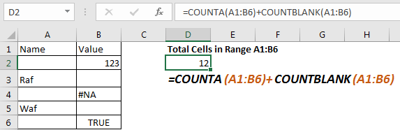
Suppose, I want to to count total number of cells in range A1:B6. We can see that it has 12 cells. Now let’s use the above formula for counting the cell in given range.
=COUNTA(A1:B6)+COUNTBLANK(A1:B6)
This formula to get cell count in range returns the correct answer.
The problem: If you read about COUNTA function, you’ll find that it counts any cell containing anything, even a formula that returns blank. COUNTBLANK function also counts any cell which is blank, even if it is returned by a formula. Now since both functions will count same cells, the returned value will be incorrect. So, use this formula to count cells, when you are sure that no formula returns blank value.
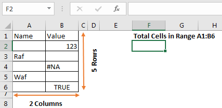
Count cells in a range using ROWS and COLUMN Function
Now, we all know that a range is made of rows and columns. Any range has at least one column and one row. So, if we multiply rows with columns, we will get our number of cell in excel range. This is same as we used to calculate the area of a rectangle.
Generic Formula to Count Cells
=ROWS(range)*COLUMNS(range)
Let’s implement this formula in above range to count cells.
=ROWS(A1:B6)*COLUMNS(A1:B6)
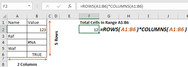
This returns the accurate number of cells in range a1:B6. It doesn’t matter what values these cells hold.
How it works
It is simple. The ROWS function, returns count of rows in range, which is 6 in this case. Similarly, COLUMN function returns the number of columns in the range, which is 2 in this example. The formula multiplies and returns the final result as 12.
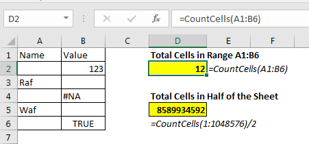
CountCells VBA Function to Count All Cells in a Range
In both of the above methods, we had to use two function of excel, and provide the same range twice. This can lead to be human error. So we can define a user defined function to count cells in a range. This is easy.
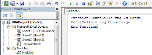
Press ALT+F11 to open VBA editor. Go to insert and click on module. Now copy below VBA code in that module.
Function CountCells(rng As Range)
CountCells = rng.CountLarge
End Function
Return to your excel file. Write CountCells function to count cells in a range. Provide range in parameter. The function will return the number of cell in the given range.
Let’s take the same example.
Write below formula to count cells in range A1:B6
=CountCells(A1:B6)
How it works
Actually, CountLarge is method of range object that counts the cell in a given range. CountCells function takes the range from user as argument and returns the cell count in range using Range.CountLarge.
This method is faster and easy to use. Once you define this function for counting cells in a range in excel, you can use it as many times as you want.
So yeah, these are the formulas to count cells in a range in excel. If you know any other ways, let us know in the comments section below.
Related Articles:
How to Count Cells that contain specific text in Excel
How to Count Unique Values In Excel
How to use the COUNT Function in Excel
How to Count Cells With Text in Excel
How to use the COUNTIFS Function in Excel
How to use the COUNTIF function in Excel
Get the Count of table rows & columns in Excel
Popular Articles :
50 Excel Shortcut to Increase Your Productivity : Get faster at your task. These 50 shortcuts will make you work even faster on Excel.
How to use the VLOOKUP Function in Excel : This is one of the most used and popular functions of excel that is used to lookup value from different ranges and sheets.
How to use the COUNTIF function in Excel : Count values with conditions using this amazing function. You don’t need to filter your data to count specific values. Countif function is essential to prepare your dashboard.
How to use the SUMIF Function in Excel : This is another dashboard essential function. This helps you sum up values on specific conditions.
There are a handful of functions that we can use to count by date, month, year, or date range in Excel 365.
We can use Excel functions such as COUNTIF, COUNTIFS, SUMPRODUCT, or combinations such as IF + SUM or COUNT + FILTER for this.
But I would pick the former two functions in Excel 365. Do you know why?
Dynamic array formulas, which spill results, are one of the main attractions in Excel in Microsoft 365.
If you are looking for a dynamic array formula to count by date, month, year, and date range in Excel 365, pick none other than COUNTIF/COUNTIFS.
So, in this tutorial, let’s learn to use COUNTIF or COUNTIFS to count by date, month, year, and date range and return an array result.
Sample Records
I have extracted a few records from my daily expense spreadsheet.
Of course, I have sanitized the data to avoid sharing personal info/preferences.
So it’s just a mockup of data in Excel 365. In that, we can try to use COUNTIF and COUNTIFS to count by date, month & year, month, year, and date range.
We will try conditions (criteria) in single (non-array) and multiple (array) rows.
At one instance, we will use a helper column, and that is for the count by month (not month and year).
Sample Data:

COUNTIF to Count by a Specific Date in Excel 365
Countif Syntax: COUNTIF(range,criteria)

Non-Array Formula (Single Date)
How to search and count the number of transactions on a particular date in the above records?
Criterion/Condition: 01/06/2020 (cell F2)
Formula:-
Insert the below Excel COUNTIF formula in cell G2 to count by the specific date, i.e., 01/06/2020.
=COUNTIF(A2:A22,F2)The above Excel formula searches F2 date in A2:A22 and returns the count, i.e., 2.
Array Formula (Multiple Dates)
Can we use multiple dates (criteria) to count in the above Excel 365 formula?
Yes. Here is how.
Criteria/Conditions: 02/06/2020 (cell F4) and 01/07/2020 (cell F5).
Formula:-
Insert the below Excel COUNTIF formula in cell G4 to count by the specific dates, i.e., 02/06/2020 and 01/07/2020. It will automatically spill in G5.
=COUNTIF(A2:A22,F4:F5)COUNTIFS to Count by Month and Year in Excel 365
COUNTIFS Syntax: COUNTIFS(criteria_range1,criteria1, ...)
The functions COUNTIF and COUNTIFS in Excel 365 won’t take other functions in their ‘range’.
So we can’t use month(range)= within these two functions.
But they support other functions in the criteria part, and we will try to benefit from that feature below.

Non-Array Formula (Month and Year)
We can use COUNTIFS to count by month and year in Excel 365.
Criterion/Condition: 6 (cell F8) and 2020 (cell G8).
Formula:-
Insert the below Excel COUNTIFS formula in cell H8 to count by the above month and year.
=COUNTIFS(A2:A22,">="&DATE(G8,F8,1),A2:A22,"<="&EOMONTH(DATE(G8,F8,1),0))The DATE(G8,F8,1) formula returns 01/06/2020, and EOMONTH(DATE(G8,F8,1)) returns the last date in that month.
The count of dates between these dates will be equal to the count by month and year.
Array Formula (Months and Years)
We can use multiple months and years (criteria) in the above Excel 365 formula.
Criteria/Conditions:
- 7 (cell F10) and 2020 (cell G10).
- 7 (cell F11) and 2021 (cell G11).
Formula:-
Insert the below Excel COUNTIFS formula in cell H10 to count by the above multiple months and years.
=COUNTIFS(A2:A22,">="&DATE(G10:G11,F10:F11,1),A2:A22,"<="&EOMONTH(DATE(G10:G11,F10:F11,1),0))Array and Non-Array COUNTIFS to Count by Year in Excel 365

Assume we have the year 2020 in cell F14.
The following COUNTIFS non-array in cell G14 returns the count by the provided year in Excel 365.
=COUNTIFS(A2:A22,">="&DATE(F14,1,1),A2:A22,"<="&DATE(F14,12,31))If the year 2020 is in cell F16 and 2021 is in cell F17, then we can use the below Excel 365 dynamic array formula in cell G16.
=COUNTIFS(A2:A22,">="&DATE(F16:F17,1,1),A2:A22,"<="&DATE(F16:F17,12,31))I hope, the above two Excel formulas are self-explanatory. Let’s move to the next example.
Array and Non-Array COUNTIFS to Count by Date Range in Excel 365
In the above examples, we have learned to count the number of transactions that have taken place on a specific date, month, and year.
But what about counting the number of transactions between two dates in Excel 365?

I wish to know how many transactions I have done during 01/06/2020 (F20) and 06/06/2020 (G20).
I can use the below Excel formula in cell H20 for that.
Count by Date Range Non-Array Formula (H20):
=COUNTIFS(A2:A22,">="&F20,A2:A22,"<="&G20)What about a count by date range array formula?
Date Range 1: F22:G22
Date Range 2: F23:G23
Count by Date Range Array Formula (H22):
=COUNTIFS(A2:A22,">="&F22:F23,A2:A22,"<="&G22:G23)Array and Non-Array COUNTIFS to Count by Month Alone in Excel 365
I know this is a rare scenario.
Usually, we may include the year component in such calculations.
For example, we will usually find the number of sales in January 2020, not in both January 2020 and January 2021.
But if you are very particular to use COUNTIFS to count by month only in Excel 365, follow the below steps.
Insert the below formula in cell D2. It will substitute the year part of the dates in cell A2:A22 with the year 2021.
=DATE(2021,MONTH(A2:A22),1)It’s a dynamic array (spill) formula. So it requires a blank range in D3:D22.
You can then hide column D or keep it.
In cell K8, enter 6 which represents June.
=COUNTIFS(D2#,">="&DATE(2021,J10,1),D2#,"<="&EOMONTH(DATE(2021,J10,1),0))The above formula in cell L8 will return the count of transactions in June. It ignores the years!
What about an array formula?
Enter 6 in K10 and 7 in K11. Then, you may insert the below formula in L10.
=COUNTIFS(D2#,">="&DATE(2021,K10:K11,1),D2#,"<="&EOMONTH(DATE(2021,K10:K11,1),0))Excel 365 Resources
- Running Count Array Formula in Excel 365.
- Array Formula to Conditional Count Unique Values in Excel 365.
- Split Function Alternative in Excel 365 with Multi-Row Support.
- How to Flatten an Array in Excel 365 Using Dynamic Formulas.
- Spill Formulas to Sum Each Row in Excel 365.