
There is one option that I always wish Excel should have, and that is counting the number of words from a cell. If you work in MS Word there is an inbuilt option on the status bar which shows you how many words are there in the sheet.

But when it comes to Excel there is no such option to count words. You can count the number of cells which have text but not actual words in them. As you know, in Excel, we have functions and you can use them to calculate almost everything. You can create a formula that can count words from a cell.
Today in this post, you will learn how to count words in Excel from a cell, a range of cells, or even the entire worksheet. And I’ll also show you how to count a specific word from a range of cells.
1. Count Words from a Single Cell
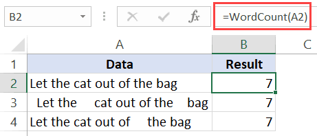
To count words from a cell you need to combine the LEN function with the SUBSTITUTE function. And the formula will be (Text is in cell A1):
=LEN(A1)-LEN(SUBSTITUTE(A1," ",""))+1
When you refer to a cell using this formula, it will return 7 in the result. And yes, you have a total of 7 words in the cell.
How it Works
Before getting into this formula just think this way. In a normal sentence if you have eight words then you will definitely have 7 spaces in those words. Right?
That means you will always have one word more than the spaces. The idea is simple: If you want to count the words, count the spaces and add one to them. To understand this formula you need to split it into three parts.

In the first part, you used the LEN function to count the number of characters from cell A1. And in the second and third parts, you have combined SUBSTITUTE with LEN to remove spaces from the cell and then count the characters. At this point, you have an equation like this.

The total number of characters with spaces and the total number of characters without spaces. And when you subtract both numbers get the number of spaces and in the end, you must add one to it. It returns 7 in the result which is the total number of words in the cell.
Important: When you use the above formula it will return 1 even if the cell is blank so it’s better to wrap it with the IF function to avoid this problem.
=IF(ISBLANK(A2),0,LEN(A2)-LEN(SUBSTITUTE(A2," ",""))+1)![]()
This formula will first check the cell and only return the word count if there is a value in the cell.
2. Using a UDF
Apart from the above formulas, I have written a small code to create a UDF for this. This code will help you to create a custom function that will simply return the word count. In short, you don’t need to combine any functions.
Function MyWordCount(rng As Range) As Integer

MyWordCount = UBound(Split(rng.Value, " "), 1) + 1

End Function
Let me tell you how to use it.
- First of all, enter this code in VBA editor.

- And then come back to your worksheet, and enter “=MyWordCount(” and refer to the cell in which you have value.

And it will return the word count.

Related: Formula Bar in Excel
3. Count Words from a Range of Cells
Now let’s come to the next level. And here you need to count words from a range of cells instead of a single cell. The good news is you just need to use the same formula (just a simple change) which you have used above. And the formula will be:
=SUMPRODUCT(LEN(A1:A11)-LEN(SUBSTITUTE(A1:A11," ",""))+1)
In the above formula, A1:A11 is the range of cells and when you enter the formula it returns 77 in the result.
How it Works
This formula works in the same way as the first method works but is just a small advance. The only difference is you have wrapped it in SUMPRODUCT and referred to the entire range instead of a single cell.
Do you know that SUMPRODUCT can take arrays? So, when you use it, it returns an array where you have a count of words for each cell. And in the end, it sums those counts and tells you the count of words in the column.
4. Word Count from the Entire Worksheet
This code is one of the useful macro codes which I use in my work, and it can help you to count all the words from a worksheet.
Sub Word_Count_Worksheet()

Dim WordCnt As Long
Dim rng As Range
Dim S As String
Dim N As Long

For Each rng In ActiveSheet.UsedRange.Cells
S = Application.WorksheetFunction.Trim(rng.Text)
N = 0

If S <> vbNullString Then
N = Len(S) – Len(Replace(S, " ", "")) + 1
End If

WordCnt = WordCnt + N

Next rng

MsgBox "There are total " & Format(WordCnt, "#,##0") & " words in the active worksheet"

End Sub
When you run it, it will show a message box with the number of words you have in the active worksheet.

Related: What is VBA in Excel
5. Count a Specific Word/Text String from a Range
Here you have a different situation. Let’s say you need to count a specific word from a range of cells or check the number of times a value appears in a column.
Take this example: Below you have a range of four cells and from this range, you need to count the count of occurrences of the word “Monday”.
For this, the formula is:
=SUMPRODUCT((LEN(D6:D9)-LEN(SUBSTITUTE(D6:D9,"Monday","")))/LEN("Monday"))
And when you enter it, it returns to the count of the word “Monday”. That’s 4.
Important: It returns the count of the word (word’s frequency) from the range not the count of the cells which have that word. Monday is there four times in three cells.
How it Works
To understand this function, again you need to split it into four parts. In the first part, the LEN function returns an array of the count of characters from the cells.

The second part returns an array of the count of characters from the cells by removing the word “Monday”.

In the third part, the LEN function returns the length of characters of wor word “Monday”.

After that, subtracts part one from part two and then divides it with part three it returns an array with the count of the word “Monday” from each cell.

In the fourth part, SUMPRODUCT returns the sum of this array and gives the count of “Monday” from the range.
Download Sample File
- Ready
Conclusion
Whenever you are typing some text in a cell or a range of cells you can these methods to keep a check on the word count. I wish someday in the future Excel will get this option to count words. But, for the time being, you have all these awesome methods.
Which method do you like the most? Make sure to share your views with me in the comment section, I’d love to hear from you. And please, don’t forget to share this post with your friends, I am sure they will appreciate it.
Want to get the word count in Excel? Believe it or not, Excel does not have an inbuilt word counter.
But don’t worry.
A cool bunch of excel functions (or a little bit of VBA if you’re feeling fancy) can easily do this for you.
In this tutorial, I will show a couple of ways to count words in Excel using simple formulas. And at the end, will also cover a technique to create a custom formula using VBA that will quickly give you the word count of any text in any cell.
Formula to Get Word Count in Excel
Before I give you the exact formula, let’s quickly cover the logic to get the word count.
Suppose I have a sentence as shown below for which I want to get the word count.
While Excel cannot count the number of words, it can count the number of spaces in a sentence.
So to get the word count, we can count these spaces instead of words and add 1 to the total (as the number of space would be one less the number of words).
Now there can be two possibilities:
- There is a single space between each word
- There are multiple spaces between words.
So let’s see how to count the total number of words in each case.
Example 1 – When there is a single space between words
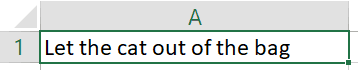
Let’s say I have the following text in cell A1: Let the cat out of the bag
To count the number of words, here is the formula I would use:
=LEN(A1)-LEN(SUBSTITUTE(A1," ",""))+1
This would return ‘7’ as a result.
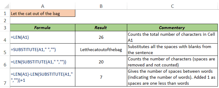
Here is how this formula works:
- LEN(A1) – This part of the formula returns 26, which is the total number of characters in the text in cell A1. It includes the text characters as well as the space characters.
- SUBSTITUTE(A1,” “,””) – This part of the formula removes all the spaces from the text. So the result, in this case, would be Letthecatoutofthebag.
- LEN(SUBSTITUTE(A1,” “,“”) – This part of the formula counts the total number of characters in the text that has no spaces. So the result of this would be 20.
- LEN(A1)-LEN(SUBSTITUTE(A1,” “,“”)) – This would subtract the text length without spaces from the text length with spaces. In the above example, it would be 26-20 which is 6.
- =LEN(A1)-LEN(SUBSTITUTE(A1,” “,“”))+1 – We add 1 to the overall result as the total number of spaces is one less than the total number of words. For example, there is one space in two words and two spaces in three words.
Now, this works well if you have only one space character between words. But it wouldn’t work if you have more than one space in between words.
In that case, use the formula in the next example.
Example 2: When there are multiple spaces between words
Let’s say you have the following text: Let the cat out of the bag
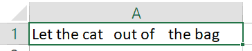
In this case, there are multiple space characters between words.
To get the word count, we first need to remove all the extra spaces (such that there is only one space character between two words) and then count the total number of spaces.
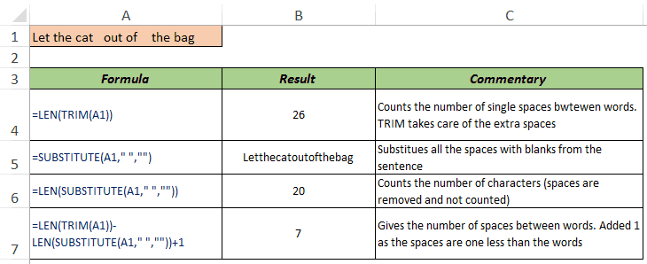
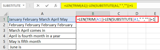
Here is the formula that will give us the right number of words:
=LEN(TRIM(A1))-LEN(SUBSTITUTE(A1," ",""))+1
This is a similar formula used in the above example, with a slight change – we have also used the TRIM function here.
Excel TRIM function removes any leading, trailing, and extra spaces (except single spaces between words).
The rest of the formula works the same (as explained in Example 1).
Note: If there are no spaces between words, it is considered as one word.
Using VBA Custom Function to Count Words in Excel
While the above formulas work great, if you have a need to calculate the word count often, you can use VBA to create a custom function (also called a User Defined Function).
The benefit of using a custom function is that you can create it once and then use it like any other regular Excel function. So instead of creating a long complex formula as we did in the two examples above, you have a simple formula that takes the cell reference and instantly gives you the word count.
Here is the code that will create this custom function to get the word count in Excel.
Function WordCount(CellRef As Range)
Dim TextStrng As String
Dim Result() As String
Result = Split(WorksheetFunction.Trim(CellRef.Text), " ")
WordCount = UBound(Result()) + 1
End Function
Once created, you can use the WordCount function just like any other regular Excel function.
In the above code for the custom function, I have used the worksheet TRIM function to remove any leading, trailing, and double spaces in between words. This ensures that all the three cells give the same result, as only the words are counted and not the double spaces.
How this formula works:
The above VBA code first uses the TRIM function to remove all the leading, trailing and double spaces from the text string in the referenced cell.
Once it has the cleaned string, it uses the SPLIT function in VBA to split the text string based on the delimiter, which we have specified to be the space character. So each word is separated as stored as a separate item in the Result variable.
We then use the UBOUND function to count the total number of items that got stored in the Result variables. Since VBA has a base of 0, we need to add 1 to get the total number of words.
This means that Result(0) stores the first word, Result(1) stores the second word, and so on. Since this counting starts from 0, we need to add 1 to get the real word count.
Where to Put this Code?
When creating a custom function, you need to put the code in the VB Editor of the workbook (which is the back end of the workbook where you can write code to automate tasks and create custom functions).
Below are the steps to put the code for the ‘GetNumeric’ function in the workbook.
- Go to the Developer tab.

- Click on Visual Basic option. This will open the VB editor in the backend.
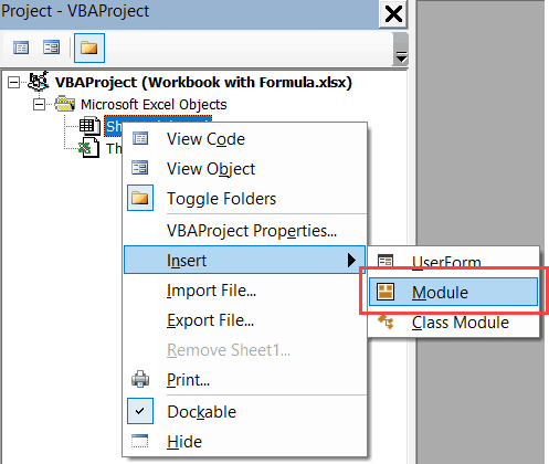
- In the Project Explorer pane in the VB Editor, right-click on any object for the workbook in which you want to insert the code. If you don’t see the Project Explorer go to the View tab and click on Project Explorer.
- Go to Insert and click on Module. This will insert a module object for your workbook.

- Copy and paste the code in the module window.
Once you have copied the code in the code window, you can go back to your worksheet and use this function just like any other regular Excel function.
Just type =Word and it will show you the formula in the list.
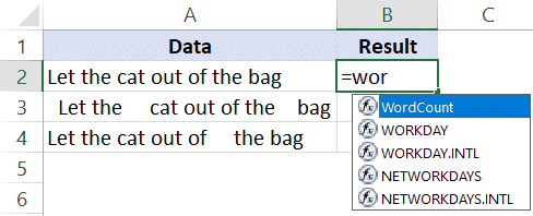
It takes one argument, which is the cell reference and instantly gives you the word count in it.
You May Also Like the Following Excel Tutorials:
- How to Count Cells that Contain Text Strings.
- Using Multiple Criteria in Excel COUNTIF and COUNTIFS Function.
- How to Add Leading Zeroes in Excel.
- Remove Spaces in Excel – Leading, Trailing, and Double.
- How to Extract the First Word from a Text String in Excel
Count Words in a Cell of Excel
There is no in-built excel formula to find the Word Count and therefore, it needs to be entered manually. You can make use of the formula below to calculate wordcount in excel –
=LEN(TRIM(cell))-LEN(SUBSTITUTE(cell,” “,””))+1
Let us understand the working of this formula.
To begin with, we utilize the SUBSTITUTE functionSubstitute function in excel is a very useful function which is used to replace or substitute a given text with another text in a given cell, this function is widely used when we send massive emails or messages in a bulk, instead of creating separate text for every user we use substitute function to replace the information.read more to evacuate and displace all spaces in the cell with a vacant content string (“). The LEN functionThe Len function returns the length of a given string. It calculates the number of characters in a given string as input. It is a text function in Excel as well as an inbuilt function that can be accessed by typing =LEN( and entering a string as input.read more restores the length of the string without spaces.
Next, we subtract the string length without spaces from the absolute length of the string. The number of words in a cell is equivalent to the number of spaces plus 1. So, we add 1 to the word count.
Further, we utilize the TRIM functionThe Trim function in Excel does exactly what its name implies: it trims some part of any string. The function of this formula is to remove any space in a given string. It does not remove a single space between two words, but it does remove any other unwanted spaces.read more to remove extra spaces in a cell. A worksheet may contain a lot of imperceptible spaces. Such coincidental occurrence might be towards the start or end of the text (leading and trailing spaces). Since extra spaces return an incorrect word count, the TRIM function is used before computing the length of the string.
The steps to count the total number of words in a cell of Excel are listed as follows:
- Select the cell in the Excel sheet where you want the result to appear.

- For counting the number of words in cell A1, enter the formula shown in the following image.

- Click “Enter” and the exact number of words appear in cell B1.


Table of contents
- Count Words in a Cell of Excel
- How to Count the Total Number of Words in a Range of Cells?
- How to Count Specific Words in a Range?
- Frequently Asked Questions
- Recommended Articles
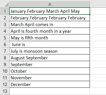
How to Count the Total Number of Words in a Range of Cells?
To count the number of words in a range of cells, apply the equation that counts the words in a cell and implant it either inside the SUM or the SUMPRODUCT function.
The formula to count words of a particular range is “=LEN(TRIM(cell))-LEN(SUBSTITUTE(cell,” “,””))+1.”
- Step 1: Select the range of data whose words you wish to count.
- Step 2: Enter the formula in the cell where you want the result to display as shown in the succeeding image.
- Step 3: Click “Enter” and the result appears in cell B1.

- Step 4: Drag the fill handle to all cells to get the word count of each cell in Excel.

How to Count Specific Words in a Range?
To count the number of times a specific word appears in a range of cells, we utilize a comparative methodology. We count the explicit words in a cell and consolidate it with the SUM or SUMPRODUCT functionThe SUMPRODUCT excel function multiplies the numbers of two or more arrays and sums up the resulting products.read more.
- Step 1: Select the cell and enter the formula “=(LEN(cell)-LEN(SUBSTITUTE(cell,word,””)))/LEN(word)” as shown in the following image.
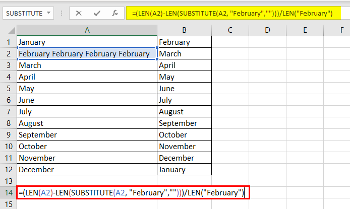
- Step 2: Click “Enter” to see the word count in cell A14. The formula we used above helps us know the number of times the word “February” is present in cell A2.
The result in cell A14 is 4.

Frequently Asked Questions
#1 – How to count the number of times a single character appears in a cell?
The formula to count the occurrence of a single character in a cell is stated as follows:
=LEN(cell_ref)-LEN(SUBSTITUTE(cell_ref,”a”,””))
The “cell_ref” stands for cell reference. The letter “a” stands for the character that the user wants to count.
#2 – How to count the number of times a single character appears in a range of cells?
The formula to count the occurrence of a single character in a range of cells is stated as follows:
=SUM(LEN(range)-LEN(SUBSTITUTE(range,”a”2,””)))
The “range” stands for the range of cells to which the formula is applied. The letter “a” stands for the character that the user wants to count.
#3 – How to count the number of times a specific word appears in a row or a column?
The steps to count the number of times a particular word appears in a row or a column are listed as follows:
1- Select the row or the column in which the word is to be counted. The row is selected by clicking the number on the left-hand side. The column is selected by clicking the letter that appears on top of the column.
2 – In the formula tab, click “Define Name” and enter a name for the row or the column in the “New Name” box.
3 – If the column is named “NamesColumn,” the cells in this column will use “NamesColumn” for reference.
4 – Apply the formula “=COUNTIF(NamesColumn,”Jack”)” to count the number of times “Jack” appears in the “NamesColumn.”
Note: Every time a new name is added to a cell of “NamesColumn,” the result of the formula will automatically update.
- The formula to count words of a particular range is “=LEN(TRIM(cell))-LEN(SUBSTITUTE(cell,” “,””))+1.”
- The word count formula is combined with the SUM or SUMPRODUCT function to handle arrays.
- The SUBSTITUTE function replaces all the spaces of the cell with a vacant content string (“).
- The LEN function restores the length of the string without spaces.
- The TRIM function removes the leading and trailing spaces found at the beginning or at the end of the text.
- The number of words in a cell is equivalent to the number of spaces plus 1.
Recommended Articles
This has been a guide to Word Count in Excel. Here we discuss how to count the total number of words in a cell and an excel range along with practical examples and a downloadable template. You may learn more about Excel from the following articles –
- Count Rows in Excel | ExamplesThere are numerous ways to count rows in Excel using the appropriate formula, whether they are data rows, empty rows, or rows containing numerical/text values. Depending on the circumstance, you can use the COUNTA, COUNT, COUNTBLANK, or COUNTIF functions.read more
- Count Colored Cells In ExcelTo count coloured cells in excel, there is no inbuilt function in excel, but there are three different methods to do this task: By using Auto Filter Option, By using VBA Code, By using FIND Method.
read more - Excel Count FormulaThe COUNT function in excel counts the number of cells containing numerical values within the given range. It is a statistical function and returns an integer value. The syntax of the COUNT formula is “=COUNT(value 1, [value 2],…)”
read more - How to Count Unique Values in Excel?In Excel, there are two ways to count values: 1) using the Sum and Countif function, and 2) using the SUMPRODUCT and Countif function.read more
- Compare Two Lists in ExcelThe five different methods used to compare two lists of a column in excel are — Compare Two Lists Using Equal Sign Operator, Match Data by Using Row Difference Technique, Match Row Difference by Using IF Condition, Match Data Even If There is a Row Difference, Partial Matching Technique.read more
no-override
Reader Interactions
Explanation
B4 is the cell we’re counting words in, and C4 contains the substring (word or any substring) you are counting.
SUBSTITUTE removes the substring from the original text and LEN calculates the length of the text without the substring. This number is then subtracted from the length of the original text. The result is the number of characters that were removed by SUBSTITUTE.
Finally, the number of characters removed is divided by the length of the substring. So, if a substring is 5 characters long, and there are 10 characters missing after it’s been removed from the original text, we know the substring appeared twice in the original text.
Handling case
SUBSTITUTE is a case-sensitive function, so it will match case when running a substitution. If you need to count both upper and lower case occurrences of a word or substring, use the UPPER function inside SUBSTITUTE to convert the text to uppercase before running the substitution:
=(LEN(B4)-LEN(SUBSTITUTE(UPPER(B4),UPPER(C4),"")))/LEN(C4)
Because this formula converts the substring and the text to uppercase before performing the substitution, it will work equally well with text in any case.
Normalizing text
Counting words in Excel is tricky because Excel doesn’t support regular expressions. As a result, it’s difficult to target the words you want to count exactly, while ignoring substrings and other partial matches (i.e. find «fox » but not «foxes»). Punctuation and case variations make this problem quite challenging.
One workaround is to use another formula in a helper column to «normalize text» as a first step. Then use the formula on this page to count words wrapped in space characters to get an accurate count (i.e. you can look for » fox » in the normalized text.
Note: this approach is only as good as the normalized text you are able to create, and you might need to adjust the normalizing formula many times to get the result you need.
Microsoft Word allows you count text, but what about Excel? If you need a count of your text in Excel, you can get this by using the COUNTIF function and then a combination of other functions depending on your desired result.
How to count text in Excel
If you want to learn how to count text in Excel, you need to use function COUNTIF with the criteria defined using wildcard *, with the formula: =COUNTIF(range;"*"). Range is defined cell range where you want to count the text in Excel and wildcard * is criteria for all text occurrences in the defined range.
Some interesting and very useful examples will be covered in this tutorial with the main focus on the COUNTIF function and different usages of this function in text counting. Limitations of COUNTIF function have been covered in this tutorial with an additional explanation of other functions such as SUMPRODUCT/ISNUMBER/FIND functions combination. After this tutorial, you will be able to count text cells in excel, count specific text cells, case sensitive text cells and text cells with multiple criteria defined – which is a very good base for further creative Excel problem-solving.
Count Text Cells in Excel
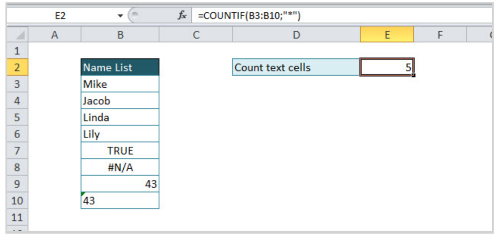
Text Cells can be easily found in Excel using COUNTIF or COUNTIFS functions. The COUNTIF function searches text cells based on specific criteria and in the defined range. As in the example below, the defined range is table Name list, and text criteria is defined using wildcard “*”. The formula result is 5, all text cells have been counted. Note that number formatted as text in cell B10 is also counted, but Booleans (TRUE /FALSE) and error (#N/A) are not recognized as text.
The formula for counting text cells:
=COUNTIF(range;"*")
For counting non-text cells, the formula should be a little bit changed in criteria part:
=COUNTIF(range;"<>*")
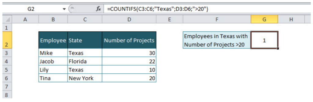
If there are several criteria for counting cells, then COUNTIFS function should be used. For example, if we want to count the number of employees from Texas with project number greater than 20, then the function will look like:
=COUNTIFS(C3:C6;"Texas";D3:D6;">20").
In criteria range in column State, a specific text criteria is defined under quotations “Texas”. The second criteria is numeric, criteria range is column Number of projects, and criteria is numeric value greater than 20, also under quotations “>20”. If we were looking for exact value, the formula would look like:
=COUNTIFS(C3:C6;"Texas";D3:D6;20)
Count Specific Text in Cells
For counting specific text under cells range, COUNTIF function is suitable with the formula:
=COUNTIF(range;"*text*")
=COUNTIF(B3:B9;"*Mike*")
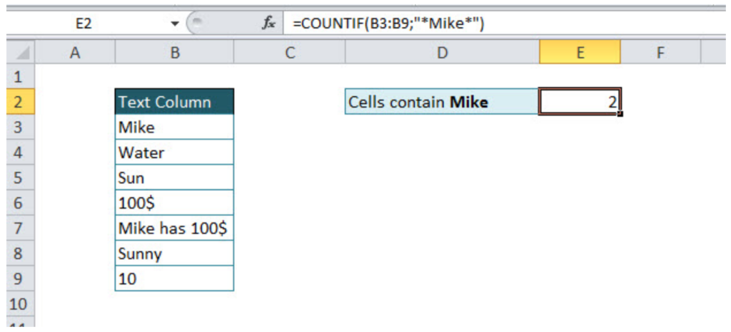
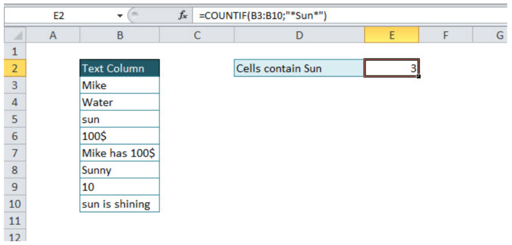
The first part of the formula is range and second is text criteria, in our example “*Mike*”. If wildcard * has not been used before and after criteria text, formula result would have been 1 (Formula would find cells only with word Mike). Wildcard * before and after criteria text, means that all cells that contain criteria characters will be taken into account. As in another example below with text criteria Sun, three cells were found (sun, Sunny, sun is shining)
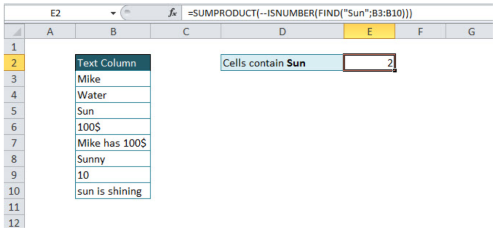
=COUNTIF(B3:B10;"*Sun*")
Note: The COUNTIF function is not case sensitive, an alternative function for case sensitive text searches is SUMPRODUCT/FIND function combination.
Count Case Sensitive Specific Text
For a case-sensitive text count, a combination of three formulas should be used: SUMPRODUCT, ISNUMBER and FIND. Let’s look in the example below. If we want to count cells that contain text Sun, case sensitive, COUNTIF function would not be the appropriate solution, instead of this function combination of three functions mentioned above has to be used.
=SUMPRODUCT(--ISNUMBER(FIND("Sun";B3:B10)))
We should go through a separate function explanation in order to understand functions combination. FIND function, searches specific text in the defined cell, and returns the number of the starting position of the text used as criteria. This explanation is relevant, if the searching range is just one cell. If we want to use FIND function in a range of the cells, then the combination with SUMPRODUCT function is necessary.
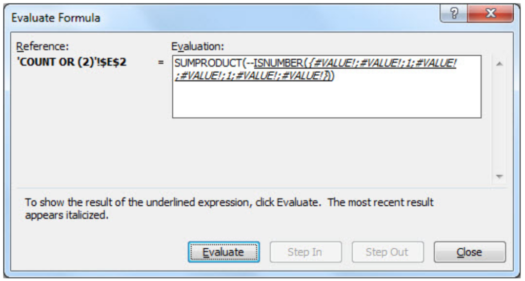
Without ISNUMBER, function combination of FIND and SUMPRODUCT functions would return an error. ISNUMBER function is necessary because whenever FIND function does not match defined criteria, the output will be an error, as in print screen below of the evaluated formula.
In order to change error values with Boolean TRUE/FALSE statement, ISNUMERIC formula should be used (defining numeric values as TRUE, and non-numeric as FALSE, as in print screen below).
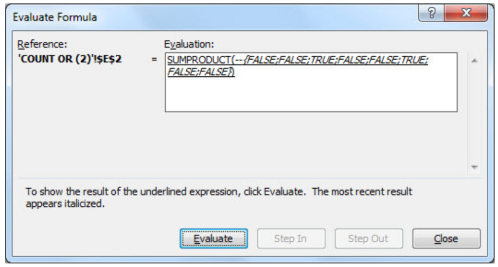
You might be wondering what character — in SUMPRODUCT function stands for. It converts Boolean values TRUE/FALSE in numeric values 1/0, enabling SUMPRODUCT function to deal with numeric operations (without character — in SUMPRODUCT function, the final result would be 0).
Remember, if you want to count specific text cells that are not case sensitive, COUNTIF function is suitable. For all case sensitive searches combination of SUMPRODUCT/ISNUMBER/FIND functions is appropriate.
Count Text Cells with Multiple Criteria
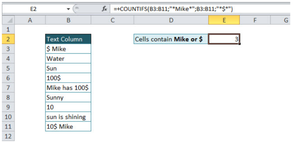
If you want to count cells with Multiple criteria, with all criteria acceptable, there is an interesting way of solving that problem, a combination of SUMPRODUCT/ISNUMBER/FIND functions. Please take a look in the example below. We should count all cells that contain either Mike or $. Tricky part could be the cells that contain both Mike and $.
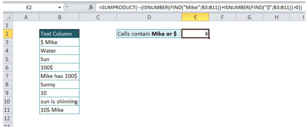
=SUMPRODUCT(--(ISNUMBER(FIND("Mike";B3:B11))+ISNUMBER(FIND("$";B3:B11))>0))
Formula just looks complex, in order to be easier for understanding, I will divide it into several steps. Also, knowledge from the previous tutorial point will be necessary for further work, since the combination of FIND, ISNUMBER, and SUMPRODUCT functions have been explained.
In the first part of the function, we loop through the table and find cells that contain Mike:
=ISNUMBER(FIND("Mike";B3:B11))
The output of this part of the function will be an array with values {1;0;0;0;1;0;0;0;1}, number 1, where criteria have been met, and 0, where has not.
In the second part of the function, looping criteria is $, counting cells containing this value:
=ISNUMBER(FIND("$";B3:B11))
The output of this part of the function will be an array with values {1;0;0;1;1;0;0;0;1}, number 1, where criteria have been met, and 0, where has not.
Next step is to sum these two arrays, since cell should be counted if any of conditions is fulfilled:
=ISNUMBER(FIND("Mike";B3:B11))+ISNUMBER(FIND("$";B3:B11))
The output of this step is {2;0;0;1;2;0;0;0;2}, the number greater than 0 means that one of the condition has been met (2 – both conditions, 1 – one condition)
Without function part >0, the final function would double count cells that met both conditions and the final result would be 7 (sum of all array numbers). In order to avoid it, in the formula should be added >0:
=ISNUMBER(FIND("Mike";B3:B11))+ISNUMBER(FIND("$";B3:B11))>0
The output of this step is array {1;0;0;1;1;0;0;0;1}, the previous array has been checked and only values greater than 0 are TRUE (in an array have value 1), and others are FALSE (in an array have value 0).
Final output of the formula is the sum of the final array values, 4.
Looks very confusing, but after several usages, you will become familiar with this functions.
At the end, we will cover one more multiple criteria text count function, already mentioned in the tutorial, COUNTIFS function. In order to distinguish the usage of functions mentioned above and COUNTIFS function, two words are enough OR/AND. If you want to count text cells with multiple criteria but all conditions have to be met at the same time, then COUNTIFS function is appropriate. If at least one condition should be met, then the combination of function explained above is suitable.
Look at the example below, the number of cells that contain both Mike and $ is easily calculated with COUNTIFS function:
=COUNTIFS(range1;"*text1*";range2;"*text2*")
=COUNTIFS(B3:B11;"*Mike*";B3:B11;"*$*")
In the defined range, function counts only cells where both conditions have been met. The final result is 3.
Still need some help with Excel formatting or have other questions about Excel? Connect with a live Excel expert here for some 1 on 1 help. Your first session is always free.