
COUNTIF Not Blank Function
The COUNTIF not blank function counts non-blank cells within a range. The universal formula is “COUNTIF(range,”<>”&””)” or “COUNTIF(range,”<>”)”. This formula works with numbers, text, and date values. It also works with the logical operators like “<,” “>,” “=,” and so on.
Note: Alternatively, the COUNTA functionThe COUNTA function is an inbuilt statistical excel function that counts the number of non-blank cells (not empty) in a cell range or the cell reference. For example, cells A1 and A3 contain values but, cell A2 is empty. The formula “=COUNTA(A1,A2,A3)” returns 2.
read more can be used to count the non-blank cells.
Table of contents
- COUNTIF Not Blank Function
- How to Use COUNTIF Non-Blank Function?
- #1–Numerical Values
- #2–Text Values
- #3–Date Values
- The Characteristics of COUNTIF Not Blank Function
- Frequently Asked Questions
- Recommended Articles
- How to Use COUNTIF Non-Blank Function?
How to Use COUNTIF Non-Blank Function?
#1–Numerical Values
The steps to count non-empty cells with the help of the COUNTIF function are listed as follows:
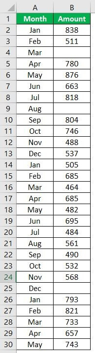
- In Excel, enter the following data containing both, the data cells and the empty cells.

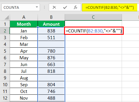
- Enter the following formula to count the data cells.
“=COUNTIF(range,”<>”&””)”
In the range argument, type B2:B30. Alternatively, select the range B2:B30 in the formula, as shown in the following image.

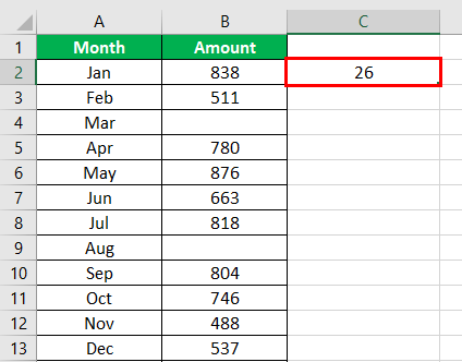
- Press the “Enter” key. The number of non-blank cells in the range B2:B30 appear in cell C2. The output is 26, as shown in the succeeding image.
This implies that there are 26 cells in the given range that contain a data value. This data can be a number, text, or any other value.

#2–Text Values
The steps to count non-empty cells within text values are listed as follows:
- Step 1: In Excel, enter the data as shown in the following image.
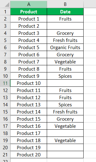
- Step 2: Select the range within which data needs to be checked for non-blank values. Enter the formula shown in the succeeding image.
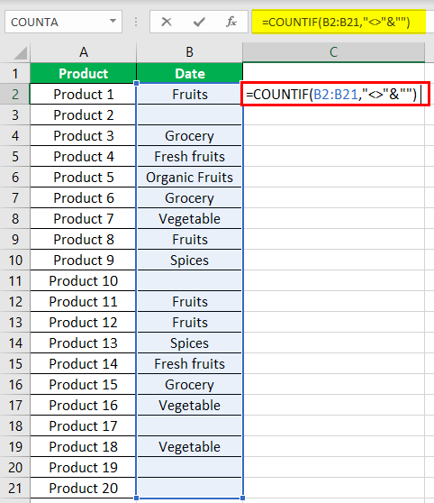
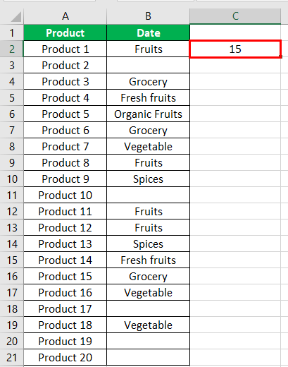
- Step 3: Press the “Enter” key. The number of non-blank cells in the range B2:B21 appear in cell C2. The output is 15, as shown in the succeeding image.
Hence, the COUNTIF not blank formula works with text values.
#3–Date Values
The steps to count non-empty cells, when the data consists of dates, are listed as follows:
- Step 1: In Excel, enter the data as shown in the following image. Select the range whose data needs to be checked for non-blank values. Enter the following formula.
“=COUNTIF(B2:B21,”<>”&””)”
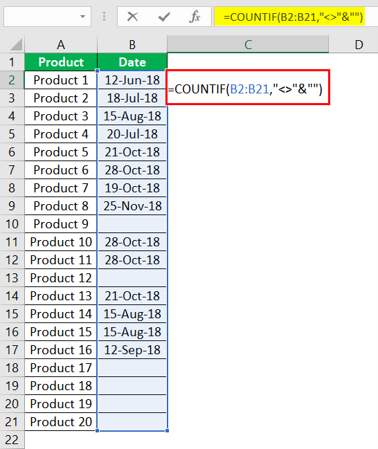
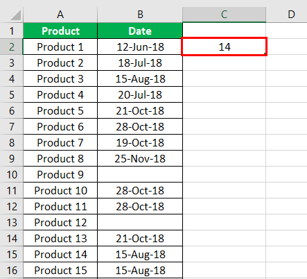
- Step 2: Press the “Enter” key. The number of non-blank cells in the range B2:B21 appear in cell C2. The output is 14, as shown in the succeeding image.
Hence, the COUNTIF not blank formula works with data that consists of date values.
The Characteristics of COUNTIF Not Blank Function
- It is case insensitive, implying that the output remains the same irrespective of whether the formula is entered in uppercase or lowercase.
- It works for data that consists of numbers, text, and date values.
- It works with greater than (>) and less than (<) operators.
- It is difficult to use the formula with long strings.
- The criteria (condition) must be specified within a pair of inverted commas to avoid errors.
Frequently Asked Questions
How is the COUNTIF formula used to count blanks?
The universal formula for counting blanks is stated as follows:
“COUNTIF(range,””)”
This formula works with all types of data values.
Note: Alternatively, the COUNTBLANK function can be used to count blank cells.
How does the COUNTIF function count the duplicate values?
The formula for counting the duplicate value is given as follows:
“COUNTIF(range,“duplicate value”)”
The “range” represents the range within which the duplicate values are to be counted. The “duplicate value” is the exact data value that is to be counted.
For example, to count the number of times the text “fruits” appears in the range A2:A10, we use “=COUNTIF(A2:A10,“fruits”).”
- The COUNTIF not blank function counts the non-blank cells within a given range.
- The generic formula of the COUNTIF not blank function is stated as–“COUNTIF (range,“<>”&””).”
- The criteria (condition) must be specified within a pair of inverted commas to avoid errors.
- The COUNTIF functionThe COUNTIF function in Excel counts the number of cells within a range based on pre-defined criteria. It is used to count cells that include dates, numbers, or text. For example, COUNTIF(A1:A10,”Trump”) will count the number of cells within the range A1:A10 that contain the text “Trump”
read more works for data that consists of numbers, text, and date values. - The COUNTIF formula gives the same output irrespective of whether the formula is entered in uppercase or lowercase.
Recommended Articles
This has been a guide to Excel COUNTIF not blank. Here we discuss how to use the COUNTIF function to count non-blank cells along with practical examples and a downloadable Excel template. You may learn more about Excel from the following articles –
- Not Equal in VBA
- COUNTIF with Multiple Criteria
- VLOOKUP Errors
- Use Not Equal to in Excel
- XML in Excel
In this example, the goal is to count cells in a range that are not blank (i.e. not empty). There are several ways to go about this task, depending on your needs. The article below explains different approaches.
COUNTA function
While the COUNT function only counts numbers, the COUNTA function counts both numbers and text. This means you can use COUNTA as a simple way to count cells that are not blank. In the example shown, the formula in F6 uses COUNTA like this:
=COUNTA(C5:C16) // returns 9
Since there are nine cells in the range C5:C16 that contain values, COUNTA returns 9. COUNTA is fully automatic, so there is nothing to configure.
COUNTIFS function
You can also use the COUNTIFS function to count cells that are not blank like this:
=COUNTIFS(C5:C16,"<>") // returns 9
The «<>» operator means «not equal to» in Excel, so this formula literally means count cells not equal to nothing. Because COUNTIFS can handle multiple criteria, we can easily extend this formula to count cells that are not empty in Group «A» like this:
=COUNTIFS(B5:B16,"A",C5:C16,"<>") // returns 4
The first range/criteria pair selects cells that are in Group A only. The second range/criteria pair selects cells that are not empty. The result from COUNTIFS is 4, since there are 4 cells in Group A that are not empty. You can swap the order of the range/criteria pairs with the same result.
See also: 50 examples of formula criteria.
SUMPRODUCT function
One problem with COUNTA and COUNTIFS is that they will also count empty strings («») returned by formulas as not blank, even though these cells are intended to be blank. For example, if A1 contains 21, this formula in B1 will return an empty string:
=IF(A1>30,"Overdue","")However, COUNTA and COUNTIFS will still count B1 as not empty. If you run into this problem, you can use the SUMPRODUCT function to count cells that are not blank like this:
=SUMPRODUCT(--(C5:C16<>""))

The expression C5:C16<>»» returns an array that contains 12 TRUE and FALSE values, and the double negative (—) converts the TRUE and FALSE values to 1s and 0s:
=SUMPRODUCT({1;1;0;1;1;0;1;1;1;0;1;1}) // returns 9
The result is 9 as before. But this formula will also ignore cells that contain formulas that return empty strings.
You can easily extend the logic used in SUMPRODUCT with other functions as needed. For example, the variant below uses the LEN function to count cells that have a length greater than zero:
=SUMPRODUCT(--(LEN(C5:C16)>0)) // returns 9
You can extend the formula to count cells that are not blank in Group A like this:
=SUMPRODUCT((LEN(C5:C16)>0)*(B5:B16="A"))
This is an example of using Boolean algebra in a formula. The double negative is no longer needed in this case because the math operation of multiplying the two arrays together automatically converts the TRUE and FALSE values to 1s and 0s:
=SUMPRODUCT({1;1;0;1;1;0;0;0;0;0;0;0}) // returns 4
The final result is 4, since there are four cells in Group A that are not blank in C5:C16.
Note: one reason the Boolean syntax above is useful is because you can drop the same logical expressions into a newer function like the FILTER function to extract cells that meet the same criteria. The SUMPRODUCT function is more versatile than RACON functions like COUNTIFS, SUMIFS, etc. and you will often see it used in formulas that solve tricky problems. You can read more about SUMPRODUCT here.
Excel for Microsoft 365 Excel for the web Excel 2021 Excel 2019 Excel 2016 Excel 2013 Excel 2010 More…Less
Suppose you need to know if your team members have entered all their project hours in a worksheet. In other words, you need to count the cells that have data. And to complicate matters, the data may not be numeric. Some of your team members may have entered placeholder values such as «TBD». For that, use the COUNTA function.
Here’s an example:
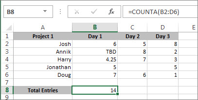
The function counts only the cells that have data, but be aware that «data» can include spaces, which you can’t see. And yes, you could probably count the blanks in this example yourself, but imagine doing that in a big workbook. So, to use the formula:
-
Determine the range of cells you want to count. The example above used cells B2 through D6.
-
Select the cell where you want to see the result, the actual count. Let’s call that the result cell.
-
In either the result cell or the formula bar, type the formula and press Enter, like so:
=COUNTA(B2:B6)
You can also count the cells in more than one range. This example counts cells in B2 through D6, and in B9 through D13.
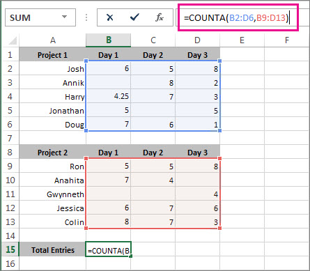
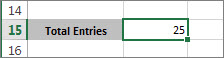
You can see Excel highlights the cells ranges, and when you press Enter, the result appears:
If you know you don’t need to count text data, just numbers and dates, use the COUNT function.
More ways to count cells that have data
-
Count characters in cells
-
Count how often a value occurs
-
Count unique values among duplicates
Need more help?
This is going to be a super simple post, here our aim is to find the number of cells that contain data, cells that are blank or empty should be excluded. The task is quite simple but the question becomes ‘how to do it?’. You know you want Excel to count a certain type of cells for you but if you find yourself wondering what to put in your sheets to get that count, you’re about to find out.
This tutorial will walk you through the usage of functions to count non-blank cells and at the end, we will also see a few functions to selectively count only the blank cells. So, without further ado, let’s jump right in.
 1")
Counting Cells That Are Not Blank
Here we are going to talk about three Excel functions that can help us to count non-blank cells from a range.
Using COUNTIF Function
The COUNTIF function counts the number of cells within a range that meet the given criteria. COUNTIF asks for the range from which it needs to count and the criteria according to which it needs to count. To count all the non-blank cells with COUNTIF we can make use of the following formula:
=COUNTIF(range,"<>")
Let’s try to understand this with an example. So, we have a dataset as shown below:
 2")
From this list of product discounts, we will aim to find how many products are discounted. In Excel’s terminology, this means – we are finding out how many non-blank cells there are in column D (the non-blank cells represent the discounts on products and the blank cells represent products with no discount).
We can easily accomplish this using the following COUNTIF formula:
=COUNTIF(D3:D14,"<>")
And our final result looks something like this.
 3")
Here, the formula has been fed with the range of column D (D3:D14). The criteria for searching column D is «<>» which is the indicator for non-blank cells («» for blank cells).
The COUNTIF function has counted 8 non-blank cells as the result. This tells us that in our dataset, there are 8 products on discount.
The COUNTIF function can be used for only one condition. For multiple conditions (e.g., non-blank cells and discount more than 20%), we can use the COUNTIFS function.
The next function we will use to count if not blank cells are present in a range is the COUNTA function.
Using COUNTA Function
By its nature, the COUNTA function counts the cells in a range that are not empty. It is a single argument function (in its simplest form) requiring just the range from which to count non-blank cells.
We will use it in our last example and simply add our range D3:D14 to the COUNTA function in this way:
=COUNTA(D3:D14)
We have the same results as the COUNTIF function i.e., 8 non-blank cells, with fewer arguments.
 4")
For the sole purpose of counting non-blank cells, the COUNTA function offers an easy, straightforward solution.
However, the COUNTA and COUNTIF functions will also count cells with space characters and formulas that return an empty string. This means that the functions will count cells that look blank but are not essentially blank.
Why is that a problem?
Technically, a space character or a formula that returns an empty string is very different from a blank cell. Although they look similar but technically they are two different things.
But since our purpose here is to count non-blank cells, so we might want the cells that appear blank to be counted as blank cells (technically, even though they are not blank). To accomplish this instead of using the COUNTIF or COUNTA functions it is better to use a SUMPRODUCT function. And this is what we are going to see in the next section.
Tip: If you are adamant about using the COUNTIF or COUNTA function for counting non-blank cells, another way around it would be to filter the data and get rid of the cells with hidden values. This will refine the results without the inclusion of faux blank cells. For now, we will move onto the SUMPRODUCT function.
Using SUMPRODUCT Function
The SUMPRODUCT returns the sum of the products of the supplied ranges or arrays. To count non-blank cells using SUMPRODUCT function we can use the below formula:
=SUMPRODUCT(--(C2:C13<>""))
Let’s try to understand the formula first and then we can compare it with the COUNTIF and COUNTA functions.
In the above formula, first of all, we are checking if the values in the range C2:C13 are equal to an empty string (nothing). This returns an array of boolean values like this –
=SUMPRODUCT(--({TRUE, TRUE, TRUE, FALSE, TRUE, TRUE, TRUE, TRUE, FALSE, TRUE, TRUE, TRUE}))
Now, since the SUMPRODUCT function cannot sum boolean values we are converting them to 0’s and 1’s by using the double-negatives. So, the formula gets further simplified to something like this –
=SUMPRODUCT({1, 1, 1, 0, 1, 1, 1, 1, 0, 1, 1, 1})
The SUMPRODUCT function adds all these 1’s and 0’s and returns the final result.
An important thing worth noting here is that the above formula does not treat space character as an empty string (nothing) so it will still be counted as a non-blank cell. To count them as blanks we can make use of the TRIM function and the final formula would look like this –
=SUMPRODUCT(--(TRIM(C2:C13)<>""))
Pro Tip: Instead of using the double negatives to convert boolean values to 1’s and 0’s we can also either add 0 to them or multiply them by 1 and our final result would still be the same.
Now, Let’s have the COUNTIF, COUNTA, and SUMPRODUCT functions side by side and analyze them:
 5")
What we can see from the serial numbering, is that there are 12 rows in our dataset. C5 is a blank cell that is correctly interpreted as blank cells by COUNTIF and COUNTA. It appears that there are 2 more blank cells (C8 containing a space character and C10 containing a formula that returns an empty string i.e., =»») in the range which means that there are 9 non-blank cells.
While the COUNTIF and COUNTA functions have treated C5 as a blank cell but they treat the other two C8 and C10 as non-blank cells and thus return 11 as the count.
On the other hand, the SUMPRODUCT based formula correctly identifies all such cells and hence returns 9 as the count of non-blank cells.
Recommended Reading: Counting Unique Values In Excel
Counting Blank Cells
Now is the turn for counting blank cells. We have ahead 2 very simple ways of counting empty cells with help of the COUNTBLANK and the COUNTIF function.
Using COUNTBLANK Function
The COUNTBLANK function, pretty self-explanatory, counts the number of empty/blank cells in a specified range. We will use the function plainly to get our results:
=COUNTBLANK(D3:D14)
 6")
We have inserted the range D3:D14 in the formula to see how many blank cells there are in column D which will tell us the number of products with no discount. The outcome of the COUNTBLANK function is «4» blank cells.
Using COUNTIF Function
As explained above, the COUNTIF function can be used for counting both, blank and non-blank cells. Now we will see how to use COUNTIF for counting blank cells.
To count blank cells the COUNTIF function can be used as:
=COUNTIF(D3:D14,"")
 7")
In the formula, which is made up of the range and criteria, we have swapped the criteria for counting non-blank cells (i.e., «<>») with the criteria for counting blank cells (i.e., «»). With the range specified as D3:D14, the COUNTIF function returns «4» blank cells as the result, indicating 4 undiscounted products.
At the end of this tutorial, we hope you won’t feel blank when trying to count if not blank and blank cells. We’re following up with more how-to’s as you read!
Author: Oscar Cronquist Article last updated on January 08, 2023
![]()
The COUNTIF function is very capable of counting non-empty values, I will show you how in this article. Excel can also highlight empty cells using Conditional formatting.
I will discuss and demonstrate the limitations of using the COUNTIF function and other equivalent functions that you also can use.
What’s on this page
- Count not blank cells — COUNTIF function
- Count not blank cells — COUNTA function
- COUNTIF and COUNTA function return unexpected results
- Count not blank cells — SUMPRODUCT function
- Get Excel *.xlsx file
1. Count not blank cells — COUNTIF function
![]()
Column B above has a few blank cells, they are in fact completely empty.
Formula in cell D3:
=COUNTIF(B3:B13,»<>»)
The first argument in the COUNTIF function is the cell range where you want to count matching cells to a specific value, the second argument is the value you want to count.
COUNTIF(range, criteria)
In this case, it is «<>» meaning not equal to and then nothing, so the COUNTIF function counts the number of cells that are not equal to nothing. In other words, cells that are not empty.

Back to top
2. Count not blank cells — COUNTA function
![]()
The COUNTA function is even easier to use, you don’t need to enter more than the cell range in one argument. The COUNTA function is designed to count non-empty cells.
COUNTA(value1, [value2], …)
Formula in cell D4:
=COUNTA(B3:B13)
Back to top
3. COUNTIF and COUNTA function return unexpected results
![]()
There are, however, situations where the COUNTIF and COUNTA function return unexpected results if you are not aware of how they work.
There are blank cells in column C, shown in the picture above, that look empty but they are not. Column D shows what they actually contain and column E shows the character length of the content.
Cell C5 and C9 contain a formula that returns a blank, both the COUNTIF and the COUNTA function count those cells as non-empty.
Cell C8 has two space characters and cell C12 has one space character, column E reveals their existence by counting character length. The COUNTIF and the COUNTA function count those cells as non-empty as well.
Back to top
4. Count not blank cells — SUMPRODUCT function
![]()
The following formula counts all non-empty values in cell range C3:C13 except formulas that return nothing. It checks if the values in cell range C3:C13 are not equal to nothing.
Formula in cell B16:
=SUMPRODUCT((C3:C13<>»»)*1)
Back to top
4.1 Explaining formula in cell B16
Step 1 — Check if cells are not empty
In this case, the logical expression counts cells that contain space characters but not formulas that return nothing.
The less than and the greater than characters are logical operators, the result are always boolean values.
C3:C13<>»»
returns
{TRUE; TRUE; FALSE; TRUE; TRUE; TRUE; FALSE; TRUE; TRUE; TRUE; TRUE}
Step 2 — Convert boolean values
The SUMPRODUCT function can’t sum boolean values, we need to multiply with one to create an array containing 0’s (zero) and 1’s.
They are their numerical equivalents:
True = 1
FALSE = 0 (zero)
(C3:C13<>»»)*1
becomes
{TRUE; TRUE; FALSE; TRUE; TRUE; TRUE; FALSE; TRUE; TRUE; TRUE; TRUE}*1
and returns
{1; 1; 0; 1; 1; 1; 0; 1; 1; 1; 1}
Step 3 — Sum numbers
Why use the SUMPRODUCT function and not the SUM function? The SUMPRODUCT function can perform calculations in the arguments without the need to enter the formula as an array formula.
Array formulas are great but if possible avoid as much as you can. Excel 365 users don’t have this problem, dynamic array formulas are entered as regular formulas.
SUMPRODUCT((C3:C13<>»»)*1)
becomes
SUMPRODUCT({1; 1; 0; 1; 1; 1; 0; 1; 1; 1; 1})
and returns 9 in cell B16.
Back to top
5. Regard formulas that return nothing to be blank and space characters to also be blank
![]()
The formula above in cell C16 counts only non-empty values, it considers formulas that return nothing to be blank and space characters to also be blank. This is made possible by the TRIM function that removes leading and ending space characters.
=SUMPRODUCT((TRIM(C3:C13)<>»»)*1)
Back to top
5.1 Explaining formula in cell B16
Step 1 — Remove space characters
TRIM(C3:C13)
returns
{«Green»; «Blue»; «»; «Red»; «Cyan»; «»; «»; «Yellow»; «Orange»; «»; «Brown»}
Step 2 — Identify not blank cells
TRIM(C3:C13)<>»»
becomes
{«Green»; «Blue»; «»; «Red»; «Cyan»; «»; «»; «Yellow»; «Orange»; «»; «Brown»}<>»»
and returns
{TRUE; TRUE; FALSE; TRUE; TRUE; FALSE; FALSE; TRUE; TRUE; FALSE; TRUE}
Step 3 — Multiply with 1
TRIM(C3:C13)<>»»)*1
becomes
{TRUE; TRUE; FALSE; TRUE; TRUE; FALSE; FALSE; TRUE; TRUE; FALSE; TRUE}*1
and returns
{1; 1; 0; 1; 1; 0; 0; 1; 1; 0; 1}
Step 4 — Sum numbers in array
SUMPRODUCT((TRIM(C3:C13)<>»»)*1)
becomes
SUMPRODUCT({1; 1; 0; 1; 1; 0; 0; 1; 1; 0; 1})
and returns 7.
Back to top
Latest updated articles.
More than 300 Excel functions with detailed information including syntax, arguments, return values, and examples for most of the functions used in Excel formulas.
More than 1300 formulas organized in subcategories.
Excel Tables simplifies your work with data, adding or removing data, filtering, totals, sorting, enhance readability using cell formatting, cell references, formulas, and more.
Allows you to filter data based on selected value , a given text, or other criteria. It also lets you filter existing data or move filtered values to a new location.
Lets you control what a user can type into a cell. It allows you to specifiy conditions and show a custom message if entered data is not valid.
Lets the user work more efficiently by showing a list that the user can select a value from. This lets you control what is shown in the list and is faster than typing into a cell.
Lets you name one or more cells, this makes it easier to find cells using the Name box, read and understand formulas containing names instead of cell references.
The Excel Solver is a free add-in that uses objective cells, constraints based on formulas on a worksheet to perform what-if analysis and other decision problems like permutations and combinations.
An Excel feature that lets you visualize data in a graph.
Format cells or cell values based a condition or criteria, there a multiple built-in Conditional Formatting tools you can use or use a custom-made conditional formatting formula.
Lets you quickly summarize vast amounts of data in a very user-friendly way. This powerful Excel feature lets you then analyze, organize and categorize important data efficiently.
VBA stands for Visual Basic for Applications and is a computer programming language developed by Microsoft, it allows you to automate time-consuming tasks and create custom functions.
A program or subroutine built in VBA that anyone can create. Use the macro-recorder to quickly create your own VBA macros.
UDF stands for User Defined Functions and is custom built functions anyone can create.
A list of all published articles.