Count days from date excel

This article describes the formula syntax and usage of the DAYS function in Microsoft Excel. For information about the DAY function, see DAY function.

Description

Returns the number of days between two dates.

Syntax

DAYS(end_date, start_date)

The DAYS function syntax has the following arguments.

• End_date    Required. Start_date and End_date are the two dates between which you want to know the number of days.

• Start_date   
  Required. Start_date and End_date are the two dates between which you want to know the number of days.

Note: Excel stores dates as sequential serial numbers so that they can be used in calculations. By default, Jan 1, 1900 is serial number 1, and January 1, 2008 is serial number 39448 because it is 39447 days after January 1, 1900.

Remarks

• If both date arguments are numbers, DAYS uses EndDate–StartDate to calculate the number of days in between both dates.

• If either one of the date arguments is text, that argument is treated as DATEVALUE(date_text) and returns an integer date instead of a time component.

• If date arguments are numeric values that fall outside the range of valid dates, DAYS returns the #NUM! error value.

• If date arguments are strings that cannot be parsed as valid dates, DAYS returns the #VALUE! error value.

Example

Copy the example data in the following table, and paste it in cell A1 of a new Excel worksheet. For formulas to show results, select them, press F2, and then press Enter. If you need to, you can adjust the column widths to see all the data.

Data
31-DEC-2021
1-JAN-2021
Formula	Description	Result
=DAYS(«15-MAR-2021″,»1-FEB-2021»)	Finds the number of days between the end date (15-MAR-2021) and start date (1-FEB-2021). When you enter a date directly in the function, you need to enclose it in quotation marks. Result is 42.	42
=DAYS(A2,A3)	Finds the number of days between the end date in A2 and the start date in A3 (364).	364

Top of Page

Date yes Add (Subtract) Days to a Date Concatenate Dates Convert Date to Number Convert Date to Text Month Name to Number Create Date Range from Dates Day Number of Year Month Name from Date First Day of Month Add (Subtract) Weeks to a Date If Functions with Dates Max Date Number of Days Between Dates Number of Days in a Month Number of Weeks Between Dates Number of Years Between Dates Split Date & Time into Separate Cells Countdown Remaining Days Insert Dates Random Date Generator Using Dynamic Ranges — Year to Date Values Add (Subtract) Years to a Date Date Formula Examples Extract Day from Date Get Day Name from Date Count Days Left in Month / Year Count Workdays Left in Month / Year Get Last Day of Month Last Business Day of Month / Year Number of Work / Business Days in Month Weekday Abbreviations Auto Populate Dates Number of Months Between Dates Quarter from a Date Years of Service Change Date Format Compare Dates Time yes Add (Subtract) Hours to Time Add (Subtract) Minutes to Time Add (Subtract) Seconds to Time Add Up time (Total Time) Time Differences Change Time Format Convert Minutes to Hours Convert Time to Decimal Convert Time to Hours Convert Time to Minutes Convert Time to Seconds Military Time Round Time to Nearest 15 Minutes Overtime Calculator Number of Hours Between Times Convert Seconds to Minutes, Hours, or Time Count Hours Worked Time Differences Time Format — Show Minutes Seconds Text yes Add Commas to Cells Get First Word from Text Capitalize First Letter Clean & Format Phone #s Remove Extra Trailing / Leading Spaces Add Spaces to Cell Assign Number Value to Text Combine Cells with Comma Combine First and Last Names Convert Text String to Date Convert Text to Number Extract Text From Cell Get Last Word Remove Unwated Characters Extract Text Before or After Character How to Split Text String by Space, Comma, & More Remove Special Characters Remove First Characters from Left Substitute Multiple Values Switch First & Last Names w/ Commas Remove Specific Text from a Cell Extract Text Between Characters (Ex. Parenthesis) Add Leading Zeros to a Number Remove Line Breaks from Text Remove all Numbers from Text Reverse Text Remove Non-Numeric Characters Remove Last Character(s) From Right Separate First and Last Names Separate Text & Numbers Round yes Round Formulas Round Price to Nearest Dollar or Cent Round to Nearest 10, 100, or 1000 Round to Nearest 5 or .5 Round Percentages Round to Significant Figures Count yes Count Blank and Non-blank Cells Count Cells Between Two Numbers Count Cells not Equal to Count if Cells are in Range Count Times Word Appears in Cell Count Words in Cell Count Specific Characters in Column Count Total Number of Characters in Column Count Cells that Equal one of two Results Count Cells that do not Contain Count Cells that Contain Specific Text Count Unique Values in Range Countif — Multiple Criteria Count Total Number of Cells in Range Count Cells with Any Text Count Total Cells in a Table Lookup yes Two Dimensional VLOOKUP VLOOKUP Simple Example Vlookup — Multiple Matches Case Sensitive Lookup Case Sensitive VLOOKUP Sum if — VLOOKUP Case Sensitive Lookup Case Sensitive VLOOKUP Find Duplicates w/ VLOOKUP or MATCH INDEX MATCH MATCH Lookup — Return Cell Address (Not Value) Lookup Last Value in Column or Row Reverse VLOOKUP (Right to Left) Risk Score Bucket with VLOOKUP Sum with a VLOOKUP Function VLOOKUP & INDIRECT VLOOKUP Concatenate VLOOKUP Contains (Partial Match) 17 Reasons Why Your XLOOKUP is Not Working Double (Nested) XLOOKUP — Dynamic Columns IFERROR (& IFNA) XLOOKUP Lookup Min / Max Value Nested VLOOKUP Top 11 Alternatives to VLOOKUP (Updated 2022!) VLOOKUP – Dynamic Column Reference VLOOKUP – Fix #N/A Error VLOOKUP – Multiple Sheets at Once VLOOKUP & HLOOKUP Combined VLOOKUP & MATCH Combined VLOOKUP Between Worksheets or Spreadsheets VLOOKUP Duplicate Values VLOOKUP Letter Grades VLOOKUP Return Multiple Columns VLOOKUP Returns 0? Return Blank Instead VLOOKUP w/o #N/A Error XLOOKUP Multiple Sheets at Once XLOOKUP Between Worksheets or Spreadsheets XLOOKUP by Date XLOOKUP Duplicate Values XLOOKUP Multiple Criteria XLOOKUP Return Multiple Columns XLOOKUP Returns 0? Return Blank Instead XLOOKUP Text XLOOKUP with IF XLOOKUP With If Statement Misc. yes Sort Multiple Columns Use Cell Value in Formula Percentage Change Between Numbers Percentage Breakdown Rank Values Add Spaces to Cell CAGR Formula Average Time Decimal Part of Number Integer Part of a Number Compare Items in a List Dealing with NA() Errors Get Worksheet Name Wildcard Characters Hyperlink to Current Folder Compound Interest Formula Percentage Increase Create Random Groups Sort with the Small and Large Functions Non-volatile Function Alternatives Decrease a Number by a Percentage Calculate Percent Variance Profit Margin Calculator Convert Column Number to Letter Get Full Address of Named Range Insert File Name Insert Path Latitute / Longitude Functions Replace Negative Values Reverse List Range Convert State Name to Abbreviation Create Dynamic Hyperlinks Custom Sort List with Formula Data Validation — Custom Formulas Dynamic Sheet Reference (INDIRECT) Reference Cell in Another Sheet or Workbook Get Cell Value by Address Get Worksheet Name Increment Cell Reference List Sheet Names List Skipped Numbers in Sequence Return Address of Max Value in Range Search by Keywords Select Every Other (or Every nth) Row Basics yes Cell Reference Basics — A1, R1C1, 3d, etc. Add Up (Sum) Entire Column or Row Into to Dynamic Array Formulas Conversions yes Convert Time Zones Convert Celsius to Fahrenheit Convert Pounds to Kilograms Convert Time to Unix Time Convert Feet to Meters Convert Centimeters to Inches Convert Kilometers to Miles Convert Inches to Feet Convert Date to Julian Format Convert Column Letter to Number Tests yes Test if a Range Contains any Text Test if any Cell in Range is Number Test if a Cell Contains a Specific Value Test if Cell Contains Any Number Test if Cell Contains Specific Number Test if Cell is Number or Text If yes Percentile If Subtotal If Sumproduct If Large If and Small If Median If Concatentate If Max If Rank If TEXTJOIN If Sum yes Sum if — Begins With / Ends With Sum if — Month or Year to Date Sum if — By Year Sum if — Blank / Non-Blank Sum if — Horizontal Sum Count / Sum If — Cell Color INDIRECT Sum Sum If — Across Multiple Sheets Sum If — By Month Sum If — Cells Not Equal To Sum If — Not Blank Sum if — Between Values Sum If — Week Number Sum Text Sum if — By Category or Group Sum if — Cell Contains Specific Text (Wildcards) Sum if — Date Rnage Sum if — Dates Equal Sum if — Day of Week Sum if — Greater Than Sum if — Less Than Average yes Average Non-Zero Values Average If — Not Blank Average — Ignore 0 Average — Ignore Errors Math yes Multiplication Table Cube Roots nth Roots Square Numbers Square Roots Calculations yes Calculate a Ratio Calculate Age KILLLLLLL Calculate Loan Payments GPA Formula Calculate VAT Tax How to Grade Formulas Find yes Find a Number in a Column / Workbook Find Most Frequent Numbers Find Smallest n Values Find nth Occurance of Character in Text Find and Extract Number from String Find Earliest or Latest Date Based on Criteria Find First Cell with Any Value Find Last Row Find Last Row with Data Find Missing Values Find Largest n Values Most Frequent Number Conditional Formatting yes Conditional Format — Dates & Times Conditional Format — Highlight Blank Cells New Functions XLOOKUP Replaces VLOOKUP, HLOOKUP, and INDEX / MATCH Logical yes AND Checks whether all conditions are met. TRUE/FALSE IF If condition is met, do something, if not, do something else. IFERROR If result is an error then do something else. NOT Changes TRUE to FALSE and FALSE to TRUE. OR Checks whether any conditions are met. TRUE/FALSE XOR Checks whether one and only one condition is met. TRUE/FALSE Lookup & Reference yes FALSE The logical value: FALSE. TRUE The logical value: TRUE. ADDRESS Returns a cell address as text. AREAS Returns the number of areas in a reference. CHOOSE Chooses a value from a list based on it’s position number. COLUMN Returns the column number of a cell reference. COLUMNS Returns the number of columns in an array. HLOOKUP Lookup a value in the first row and return a value. HYPERLINK Creates a clickable link. INDEX Returns a value based on it’s column and row numbers. INDIRECT Creates a cell reference from text. LOOKUP Looks up values either horizontally or vertically. MATCH Searches for a value in a list and returns its position. OFFSET Creates a reference offset from a starting point. ROW Returns the row number of a cell reference. ROWS Returns the number of rows in an array. TRANSPOSE Flips the oriention of a range of cells. VLOOKUP Lookup a value in the first column and return a value. Date & Time yes DATE Returns a date from year, month, and day. DATEDIF Number of days, months or years between two dates. DATEVALUE Converts a date stored as text into a valid date DAY Returns the day as a number (1-31). DAYS Returns the number of days between two dates. DAYS360 Returns days between 2 dates in a 360 day year. EDATE Returns a date, n months away from a start date. EOMONTH Returns the last day of the month, n months away date. HOUR Returns the hour as a number (0-23). MINUTE Returns the minute as a number (0-59). MONTH Returns the month as a number (1-12). NETWORKDAYS Number of working days between 2 dates. NETWORKDAYS.INTL Working days between 2 dates, custom weekends. NOW Returns the current date and time. SECOND Returns the second as a number (0-59) TIME Returns the time from a hour, minute, and second. TIMEVALUE Converts a time stored as text into a valid time. TODAY Returns the current date. WEEKDAY Returns the day of the week as a number (1-7). WEEKNUM Returns the week number in a year (1-52). WORKDAY The date n working days from a date. WORKDAY.INTL The date n working days from a date, custom weekends. YEAR Returns the year. YEARFRAC Returns the fraction of a year between 2 dates. Engineering yes CONVERT Convert number from one unit to another. Financial yes FV Calculates the future value. PV Calculates the present value. NPER Calculates the total number of payment periods. PMT Calculates the payment amount. RATE Calculates the interest Rate. NPV Calculates the net present value. IRR The internal rate of return for a set of periodic CFs. XIRR The internal rate of return for a set of non-periodic CFs. PRICE Calculates the price of a bond. YIELD Calculates the bond yield. INTRATE The interest rate of a fully invested security. Information yes CELL Returns information about a cell. ERROR.TYPE Returns a value representing the cell error. ISBLANK Test if cell is blank. TRUE/FALSE ISERR Test if cell value is an error, ignores #N/A. TRUE/FALSE ISERROR Test if cell value is an error. TRUE/FALSE ISEVEN Test if cell value is even. TRUE/FALSE ISFORMULA Test if cell is a formula. TRUE/FALSE ISLOGICAL Test if cell is logical (TRUE or FALSE). TRUE/FALSE ISNA Test if cell value is #N/A. TRUE/FALSE ISNONTEXT Test if cell is not text (blank cells are not text). TRUE/FALSE ISNUMBER Test if cell is a number. TRUE/FALSE ISODD Test if cell value is odd. TRUE/FALSE ISREF Test if cell value is a reference. TRUE/FALSE ISTEXT Test if cell is text. TRUE/FALSE N Converts a value to a number. NA Returns the error: #N/A. TYPE Returns the type of value in a cell. Math yes ABS Calculates the absolute value of a number. AGGREGATE Define and perform calculations for a database or a list. CEILING Rounds a number up, to the nearest specified multiple. COS Returns the cosine of an angle. DEGREES Converts radians to degrees. DSUM Sums database records that meet certain criteria. EVEN Rounds to the nearest even integer. EXP Calculates the exponential value for a given number. FACT Returns the factorial. FLOOR Rounds a number down, to the nearest specified multiple. GCD Returns the greatest common divisor. INT Rounds a number down to the nearest integer. LCM Returns the least common multiple. LN Returns the natural logarithm of a number. LOG Returns the logarithm of a number to a specified base. LOG10 Returns the base-10 logarithm of a number. MOD Returns the remainder after dividing. MROUND Rounds a number to a specified multiple. ODD Rounds to the nearest odd integer. PI The value of PI. POWER Calculates a number raised to a power. PRODUCT Multiplies an array of numbers. QUOTIENT Returns the integer result of division. RADIANS Converts an angle into radians. RAND Calculates a random number between 0 and 1. RANDBETWEEN Calculates a random number between two numbers. ROUND Rounds a number to a specified number of digits. ROUNDDOWN Rounds a number down (towards zero). ROUNDUP Rounds a number up (away from zero). SIGN Returns the sign of a number. SIN Returns the sine of an angle. SQRT Calculates the square root of a number. SUBTOTAL Returns a summary statistic for a series of data. SUM Adds numbers together. SUMIF Sums numbers that meet a criteria. SUMIFS Sums numbers that meet multiple criteria. SUMPRODUCT Multiplies arrays of numbers and sums the resultant array. TAN Returns the tangent of an angle. TRUNC Truncates a number to a specific number of digits. Stats yes AVERAGE Averages numbers. AVERAGEA Averages numbers. Includes text & FALSE =0, TRUE =1. AVERAGEIF Averages numbers that meet a criteria. AVERAGEIFS Averages numbers that meet multiple criteria. CORREL Calculates the correlation of two series. COUNT Counts cells that contain a number. COUNTA Count cells that are non-blank. COUNTBLANK Counts cells that are blank. COUNTIF Counts cells that meet a criteria. COUNTIFS Counts cells that meet multiple criteria. FORECAST Predict future y-values from linear trend line. FREQUENCY Counts values that fall within specified ranges. GROWTH Calculates Y values based on exponential growth. INTERCEPT Calculates the Y intercept for a best-fit line. LARGE Returns the kth largest value. LINEST Returns statistics about a trendline. MAX Returns the largest number. MEDIAN Returns the median number. MIN Returns the smallest number. MODE Returns the most common number. PERCENTILE Returns the kth percentile. PERCENTILE.INC Returns the kth percentile. Where k is inclusive. PERCENTILE.EXC Returns the kth percentile. Where k is exclusive. QUARTILE Returns the specified quartile value. QUARTILE.INC Returns the specified quartile value. Inclusive. QUARTILE.EXC Returns the specified quartile value. Exclusive. RANK Rank of a number within a series. RANK.AVG Rank of a number within a series. Averages. RANK.EQ Rank of a number within a series. Top Rank. SLOPE Calculates the slope from linear regression. SMALL Returns the kth smallest value. STDEV Calculates the standard deviation. STDEV.P Calculates the SD of an entire population. STDEV.S Calculates the SD of a sample. STDEVP Calculates the SD of an entire population TREND Calculates Y values based on a trendline. Text yes CHAR Returns a character specified by a code. CLEAN Removes all non-printable characters. CODE Returns the numeric code for a character. CONCATENATE Combines text together. DOLLAR Converts a number to text in currency format. EXACT Test if cells are exactly equal. Case-sensitive. TRUE/FALSE FIND Locates position of text within a cell.Case-sensitive. LEFT Truncates text a number of characters from the left. LEN Counts number of characters in text. LOWER Converts text to lower case. MID Extracts text from the middle of a cell. PROPER Converts text to proper case. REPLACE Replaces text based on it’s location. REPT Repeats text a number of times. RIGHT Truncates text a number of characters from the right. SEARCH Locates position of text within a cell.Not Case-sensitive. SUBSTITUTE Finds and replaces text. Case-sensitive. TEXT Converts a value into text with a specific number format. TRIM Removes all extra spaces from text. UPPER Converts text to upper case. VALUE Converts a number stored as text into a number.

Summary

The Excel DAYS function returns the number of days between two dates. With a start date in A1 and end date in B1, =DAYS(B1,A1) will return the days between the two dates.

Purpose 

Return value 

A number representing days.

Arguments 

• end_date — The end date.
• start_date — The start date.

Syntax 

=DAYS(end_date, start_date)

Usage notes 

The DAYS function returns the number of days between two dates. Both dates must be valid Excel dates or text values that can be coerced to dates. The DAYS function only works with whole numbers, fractional time values that might be part of a date are ignored. If start and end dates are reversed, DAYS returns a negative number. The DAYS function returns all days between two dates, to calculate working days between dates, see the NETWORKDAYS function.

Examples

With a start date in A1 and end date in A2:

=DAYS(A2,A1)

Will return the same result as:

=A2-A1

Unlike the simple formula above, the DAYS function can also handle dates in text format, as long as the date is recognized by Excel. For example:

=DAYS("7/15/2016","7/1/2016") // returns 14

The DAYS function returns the number of days between two dates. For example:

=DAYS("1-Mar-21","2-Mar-21") // returns 1

To include the end date in the count, add 1 to the result:

=DAYS("1-Mar-21","2-Mar-21")+1 // returns 2

Storing and parsing text values that represent dates should be avoided, because it can introduce errors and parsing problems. Working with native Excel dates (which are numbers) is a better approach. To create a numeric date from scratch in a formula, use the DATE function.

Notes

• The DAYS function only works with whole numbers and ignores time.
• If dates are not recognized, DAYS returns the #VALUE! error.
• If dates are out of range, DAYS returns the #NUM! error.

Author

Dave Bruns

Hi — I’m Dave Bruns, and I run Exceljet with my wife, Lisa. Our goal is to help you work faster in Excel. We create short videos, and clear examples of formulas, functions, pivot tables, conditional formatting, and charts.

If you want to know how to use Excel to count days between two dates, then this post is going to help you. There may be times when you need to calculate the number of days between two given dates while analyzing some financial data. Excel is an amazing tool that can do that for you in a matter of seconds. How? By using Excel Functions! Excel offers a bunch of useful functions that allow you to quickly find the count, sum, average, maximum value, minimum value, etc., for a range of cells. It also offers some text functions and financial functions that are worth checking.

In this post, we are going to show you 5 different methods to count days between two Dates in Excel. They are:

1. Using Subtraction
2. Using the DAYS function
3. Using the DATEDIF function
4. Using the NETWORKDAYS function
5. Using the TODAY function

Let us have a detailed look at all the above methods.

1] Using Subtraction

Subtraction is the easiest way to count days between two dates in Excel. You can use the arithmetic operator – (minus sign) to subtract one date from another to find the number of days between them.

Let’s say we have an Excel sheet with some sample dates listed in two columns, Column A and Column B. The dates in Column B precede the dates in Column A. The third column, Column C, will display the count of days when we subtract the value of Column A from the value of Column B, for each row in the spreadsheet.

The following steps describe the process in detail:

1. Place your cursor in cell C3.
2. In the formula bar, type =B3-A3.
3. Press the Enter key. Excel will calculate the number of days between the dates entered in cells B3 and A3 and display the result in cell C3.
4. Take your mouse pointer to the lower-right corner of cell C3. It will turn into a + (plus) symbol.
5. Click, hold, and drag the cursor till cell C6. This action will copy the formula of cell C3 to cells C4, C5, and C6 as well, displaying results for all the dates we have taken into consideration.

Note: While using Subtraction, always write the End Date before the Start Date.

2] Using the DAYS function

DAYS is a date function in Excel that calculates the difference between two given dates in days. It can recognize dates passed as ‘strings’ if they can be parsed as valid dates in Excel.

Syntax

DAYS(end_date, start_date)

• end_date is the last date provided
• start_date is the first date provided

Now for the same example described above, we can use the DAYS formula to count the days as follows:

1. Keeping the focus on cell C3, type =DAYS(B3, A3) in the formula bar.
2. Press the Enter key. Days count between dates in cells A3 and B3 will appear in C3.
3. Copy the same formula to cells C4, C5, and C6 through the mouse cursor drag method, as explained above.

Tip: If your accounting system is based on a 360-day year (twelve 30-day months), you may use the DAYS360 function to count the number of days.

3] Using the DATEDIF function

The DATEDIF function is an advanced version of the DAYS function. It calculates the difference between two date values based on a specified interval, such as days, months, or years. It is useful in formulas that involve age-based calculations.

Syntax

DATEDIF(start_date, end_date, unit)

• start_date is the first or start date of the given period.
• end_date is the last date of the given period.
• unit is the information that you would like to get. For example, if you want the DATEDIF function to calculate the number of days, you can enter D in place of the unit. Similarly, you can enter M for months and Y for years. You can also enter a combination of two units, such as YM. This will calculate the difference in months, ignoring the years and the days.

Now taking the same example as above, follow these steps to use the DATEDIF function to count days in Excel:

1. Place your cursor in cell C3.
2. Double click and type =DATEDIF(A3, B3, “D”)
3. Press the Enter key. The results will be displayed in cell C3.
4. Now again take your cursor to the lower-right corner of cell C3, and click and drag it to cell C6 to view all the results.

Also Read: How to count words in Microsoft Excel.

4] Using the NETWORKDAYS function

NETWORKDAYS is another useful function through which you can use Excel to find days between two dates. It calculates the number of whole working days between two given dates. While calculating the number of days between two given dates, it automatically excludes the weekends (Saturday, Sunday) and optionally excludes any other holidays provided as dates (state, federal, and floating holidays).

Syntax

NETWORKDAYS(start_date,end_date,[holidays])

• start_date argument takes the value of the start date.
• end_date argument takes the value of the end date.
• [holidays] is a reference to one or dates to be counted as non-working days.

Now let’s say we provide a list of holidays (other than weekends) for the same set of dates as shown in the above example. We can use the NETWORKDAYS function to calculate working days between the given dates as follow:

1. Place the cursor in cell D6.
2. In the formula bar, type =NETWORKDAYS(A6,B6,D10:D11). As you can see in the above screenshot, the count of days has now been reduced from 30 to 22 (excluding 4 Saturdays, 4 Sundays, and 1 holiday which is occurring on Sunday).
3. Now double click on cell D5 and type =NETWORKDAYS(A5,B5,D10:D11).
4. Press the Enter key. The function now returns 4, excluding 1 Sunday and 1 holiday.

Notes:

1. The NETWORKDAYS function includes the start_date in the count if it happens to be a weekday.
2. If you need to provide custom weekends (for example, if you want Excel to mark Wednesday as a weekend and not Saturday, Sunday), then you should use the NETWORKDAYS.INTL function. This function allows you to pass a ‘weekend’ argument to set which days are considered weekends.

5] Using the TODAY function

The TODAY function can be used to calculate the number of days between a past date or a future date, and the current date. By default, it returns the current date (if the cell format is set to General).

Syntax

Today()

Let’s say the current date is 28 September 2022. And we have the date value 04 September 2022 in cell A17 and the date value 30 September 2022 in cell A18.

To calculate the number of days between today and 04 September 2022 (which is a past date), we will use the formula =TODAY()-A17. The function returns 24 as the resultant value.

Similarly, to calculate the number of days between today and 30 September 2022 (which is a future date), we will use the formula =A18-TODAY(). The function returns 2 as the resultant value.

That’s it! Hope you enjoyed knowing these easy tips to use Excel to count days between two dates. Do let us know in the comments if you have any questions.

What is the formula to calculate days?

Multiple Excel formulas can be used to calculate the days between 2 given dates. These include DAYS, DATEDIF, NETWORKDAYS, and TODAY functions. To know how these functions can be used to count days, refer to the above post. You may also use the Subtraction operator (-) to count days between two dates, as explained in this post.

How do I count days from a date in Excel?

There are five ways to count days from a date in Excel. For example, you can use the simple subtraction method to get the job done. However, if it doesn’t work, you can use the DAYS, DATEIF, NETWORKDAYS, or TODAY function as well. For your information, these functions work on Excel, Excel Online, and Google Sheets.

Read Next: How to multiply numbers in Single or Multiple cells in Excel.

Итак, мы имеем несколько серьезных функций, для того чтобы рассчитать кол-во дней между двумя датами, причем с разными параметрами (такими как выходные дни, праздники и так далее).

В этой статье я продемонстрирую вам разные ситуации, где нужно посчитать кол-во дней между датами. Все они будут с разными «уклонами», в одной ситуации нужно посчитать без выходных, в другой количество понедельников и так далее.

Стандартный расчет количества дней

Итак, в Excel есть две функции для вычисления кол-ва дней.

С помощью функции ДНИ

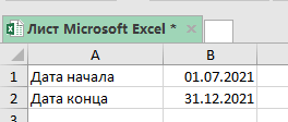
Чтобы получить результат от функции нам понадобится дата начала и дата конца.

Итак, вы указываете эти две даты в аргументах функции и получаете количество дней между ними.

Хороший пример вы можете видеть на картинке ниже:

Используем эту формулу:

=ДНИ(B2;B1)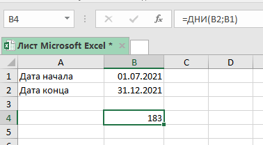  

Также вы можете вручную прописать даты в функции (без указания ячеек), но тогда вам нужно заключить их в кавычки.

Эта функция вычислит количество дней между этими датами, но если вы хотите чтобы расчет велся «включительно» с датами начала и конца, то добавьте к результату + 1 (просто пропишите это в функции).

С помощью функции РАЗНДАТ

Эта функция аналогична, её отличие в том, что можно указать больше параметров. То есть больше «подстроить» под ситуацию.

Также можно вычислить кол-во месяцев или лет между датами.

Допустим, мы имеем то что указано на картинке ниже:

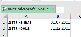
Пропишем формулу:

=РАЗНДАТ(B1;B2;"D")  

Эта функция использует три наших аргумента:

• Дата начала — B1
• Дата окончания — B2
• «D» — текстовая строка

Важный момент: этой функции не будет в подсказке при написании названия функции, т.е. если вы будете писать РАЗНДАТ, Excel будет вести себя так, как будто он не знает что это за функция, но это не так.

Функция РАЗНДАТ больше подходит для ситуаций, когда нужно вычислить кол-во лет или месяцев между датами, в других ситуациях удобнее применять ДНИ (функцию).

Вот формула, которая даст результат по месяцам, которые будут между датами:

=РАЗНДАТ(B1;B2;"M") 

А эта формула, тоже самое что и прошлая, только вычисляет кол-во лет:

=РАЗНДАТ(B1;B2;"Y")  

Расчет кол-ва рабочих дней

Итак, рабочие дни можно вычислить двумя способами:

• Функция Excel ЧИСТРАБДНИ — ее следует использовать, если выходные дни — суббота и воскресенье.
• Функция Excel ЧИСТРАБДНИ.МЕЖД — используйте ее, когда выходные дни отличаются от субботы и воскресенья.

Сначала быстро рассмотрим синтаксис и аргументы фунции ЧИСТРАБДНИ.

Функция Excel ЧИСТРАБДНИ

=ЧИСТРАБДНИ(нач_дата, конеч_дата, [праздники])

• нач_дата — это дата начала отсчета.
• end_date — это конечная дата отсчета.
• [праздники] — (Необязательно) Отдельная дата или диапазон дат, которые не будут учитываться в расчетах.

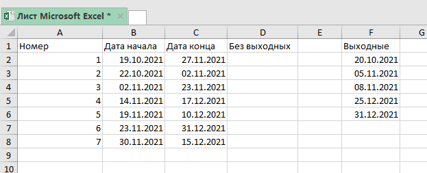
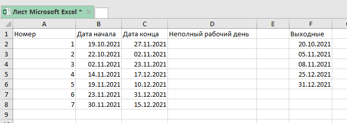
Посмотрим на стандартный пример, когда нужно посчитать кол-во рабочих дней.

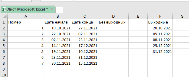
Мы будем использовать эту формулу:

=ЧИСТРАБДНИ(B2;C2;$F$2:$F$6)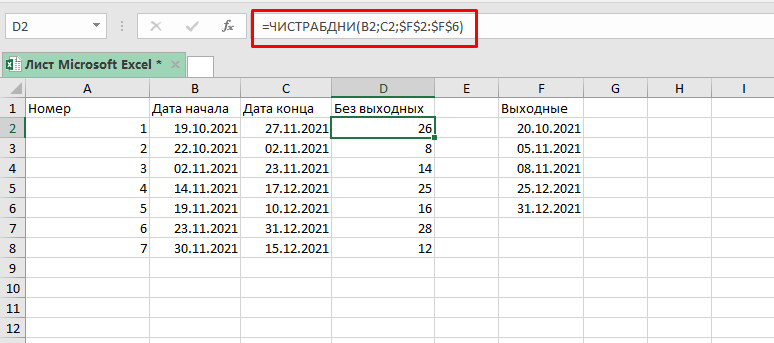  

Такая вариация этой функции даст то что вам нужно, если вам нужно посчитать рабочие дни без субботы и воскресенья.

Но бывают и другие ситуации, к примеру, в разных странах выходные на неделе строятся по-разному, это может быть пятница и так далее.

Именно для таких ситуаций и появилась функция ЧИСТРАБДНИ.МЕЖД.

Посмотрим что из себя представляет эта функция.

Функция Excel ЧИСТРАБДНИ.МЕЖД

=ЧИСТРАБДНИ.МЕЖД(нач_дата; конеч_дата; [выходные]; [праздники])

• нач_дата — значение даты, представляющее собой начальную дату.
• конеч_дата — значение даты, представляющее дату окончания.
• [нерабочие дни] — (Необязательно) в этом аргументе указываются исключительные дни(праздники и т.д.), если аргумента не будет, выходные останутся по-стандарту(суббота и воскресенье).

А сейчас, попробуем посчитать кол-во рабочих дней, если выходными будут пятница и суббота.

Допустим, таблица такая же как и в прошлом примере:

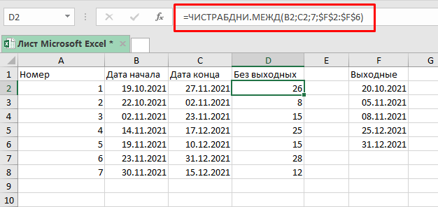
Будем использовать формулу:

=ЧИСТРАБДНИ.МЕЖД(B2;C2;7;$F$2:$F$6)  

3 аргумент в функции сообщает Excel, что пятница и суббота выходные.

Также, мы можем использовать ЧИСТРАБДНИ.МЕЖД для расчета выходных между двумя датами.

Она конечно вычисляет кол-во рабочих дней, но мы можем адаптировать это «под себя».

Допустим, таблица все та же:

Формула, которая нам подойдет:

=ДНИ(C2;B2)+1-РАЗНДАТ(B2;C2)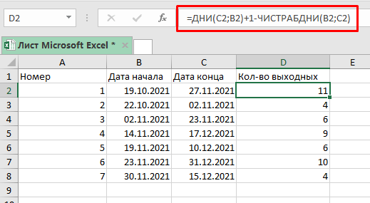

Расчет кол-ва неполных рабочих дней между двумя датами

Также, к примеру, можно использовать эту же функцию для расчета неполных рабочих дней.

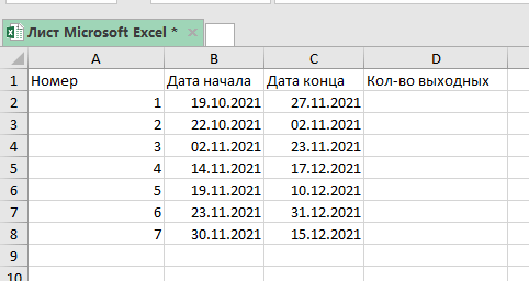
Допустим, у нас есть похожая таблица с данными:

Формула, для нашего случая, будет такой:

=ЧИСТРАБДНИ.МЕЖД($B$3;$C$3;"1010111";$E$3:$E$7)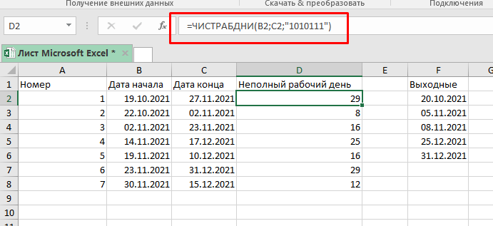  

Для обозначения выходных дней, мы использовали «1010111».

• 0 — рабочий день
• 1 — неполный рабочий день

Первая цифра из этого числа — понедельник, последняя — воскресенье

Грубо говоря, «0000011» значит, что с понедельника по пятницу — рабочие дни, а суббота и воскресенье — нерабочие (выходные).

По той же логике, «1010111» означает, что только вторник и четверг являются рабочими, а остальные 5 дней — нерабочими.

Если вам нужно исключить какие-то дни из расчетов, можете исключать их таким образом.

Количество понедельников между двумя датами

Для поиска количества понедельников мы можем использовать ту же логику, которая использовалась выше при подсчете неполных рабочих дней.

Функция, которая выведет кол-во понедельников:

=ЧИСТРАБДНИ(B2;C2;"0111111")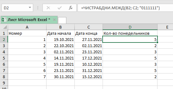  

В этой формуле «0» означает рабочий день, а «1» — нерабочий день.

Формула рассчитывает количество рабочих дней, с учетом того что единственный рабочий день — это понедельник.

Аналогичным образом можно рассчитать количество любых, интересующих вас дней, между двумя датами.