
-
— By
Sumit Bansal
Watch Video – How to Count Colored Cells in Excel
Wouldn’t it be great if there was a function that could count colored cells in Excel?
Sadly, there isn’t any inbuilt function to do this.
BUT..
It can easily be done.
How to Count Colored Cells in Excel
In this tutorial, I will show you three ways to count colored cells in Excel (with and without VBA):
- Using Filter and SUBTOTAL function
- Using GET.CELL function
- Using a Custom Function created using VBA
#1 Count Colored Cells Using Filter and SUBTOTAL
To count colored cells in Excel, you need to use the following two steps:
- Filter colored cells
- Use the SUBTOTAL function to count colored cells that are visible (after filtering).
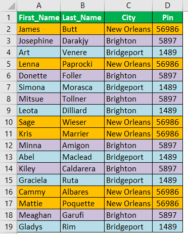
Suppose you have a dataset as shown below:

There are two background colors used in this data set (green and orange).
Here are the steps count colored cells in Excel:
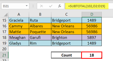
- In any cell below the data set, use the following formula: =SUBTOTAL(102,E1:E20)

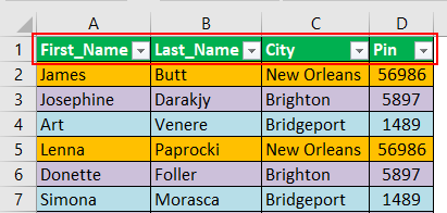
- Select the headers.
- Go to Data –> Sort and Filter –> Filter. This will apply a filter to all the headers.
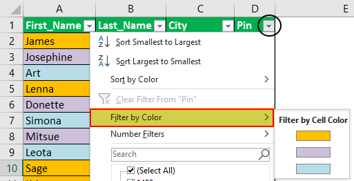
- Click on any of the filter drop-downs.
- Go to ‘Filter by Color’ and select the color. In the above dataset, since there are two colors used for highlighting the cells, the filter shows two colors to filter these cells.


As soon as you filter the cells, you will notice that the value in the SUBTOTAL function changes and returns only the number of cells that are visible after filtering.
How does this work?
The SUBTOTAL function uses 102 as the first argument, which is used to count visible cells (hidden rows are not counted) in the specified range.
If the data if not filtered it returns 19, but if it is filtered, then it only returns the count of the visible cells.
Try it Yourself.. Download the Example File

#2 Count Colored Cells Using GET.CELL Function
GET.CELL is a Macro4 function that has been kept due to compatibility reasons.
It does not work if used as regular functions in the worksheet.
However, it works in Excel named ranges.
See Also: Know more about GET.CELL function.
Here are the three steps to use GET.CELL to count colored cells in Excel:
- Create a Named Range using GET.CELL function
- Use the Named Range to get color code in a column
- Using the Color Number to Count the number of Colored Cells (by color)
Let’s deep dive and see what to do in each of the three mentioned steps.
Creating a Named Range
Getting the Color Code for Each Cell
In the cell adjacent to the data, use the formula =GetColor
This formula would return 0 if there is NO background color in a cell and would return a specific number if there is a background color.
This number is specific to a color, so all the cells with the same background color get the same number.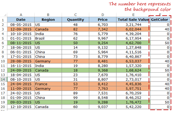
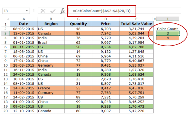
Count Colored Cells using the Color Code
If you follow the above process, you would have a column with numbers corresponding to the background color in it.
To get the count of a specific color:
- Somewhere below the dataset, give the same background color to a cell that you want to count. Make sure you are doing this in the same column that you used in creating the named range. For example, I used Column A, and hence I will use the cells in column ‘A’ only.
- In the adjacent cell, use the following formula:
=COUNTIF($F$2:$F$20,GetColor)
This formula will give you the count of all the cells with the specified background color.
How Does It Work?
The COUNTIF function uses the named range (GetColor) as the criteria. The named range in the formula refers to the adjacent cell on the left (in column A) and returns the color code for that cell. Hence, this color code number is the criteria.
The COUNTIF function uses the range ($F$2:$F$18) which holds the color code numbers of all the cells and returns the count based on the criteria number.
Try it Yourself.. Download the Example File
#3 Count Colored Using VBA (by Creating a Custom Function)
In the above two methods, you learned how to count colored cells without using VBA.
But, if you are fine with using VBA, this is the easiest of the three methods.
Using VBA, we would create a custom function, that would work like a COUNTIF function and return the count of cells with the specific background color.
Here is the code:
'Code created by Sumit Bansal from https://trumpexcel.com
Function GetColorCount(CountRange As Range, CountColor As Range)
Dim CountColorValue As Integer
Dim TotalCount As Integer
CountColorValue = CountColor.Interior.ColorIndex
Set rCell = CountRange
For Each rCell In CountRange
  If rCell.Interior.ColorIndex = CountColorValue Then
    TotalCount = TotalCount + 1
  End If
Next rCell
GetColorCount = TotalCount
End Function
To create this custom function:
To use this function, simply use it as any regular excel function.
Syntax: =GetColorCount(CountRange, CountColor)
- CountRange: the range in which you want to count the cells with the specified background color.
- CountColor: the color for which you want to count the cells.
To use this formula, use the same background color (that you want to count) in a cell and use the formula. CountColor argument would be the same cell where you are entering the formula (as shown below):
Note: Since there is a code in the workbook, save it with a .xls or .xlsm extension.
Try it Yourself.. Download the Example File
Do you know any other way to count colored cells in Excel?
If yes, do share it with me by leaving a comment.
You May Also Like the Following Excel Tutorials:
- Count Cells that Contain Text
- How to Sum by Color in Excel (Formula & VBA)
- Filter Cells with Bold Font Formatting
- How to Format Partial Text Strings using VBA
- Highlight EVERY Other ROW in Excel (using conditional formatting).
- How to Quickly Highlight Blank Cells in Excel.
- How to Compare Two Columns in Excel.

Get 51 Excel Tips Ebook to skyrocket your productivity and get work done faster
67 thoughts on “How to Count Colored Cells in Excel – A Step by Step Tutorial + Video”
-
I’m noticing that the VBA method doesn’t work with conditional formatting of background colors. Any workaround for hat?
-
I have the same issue
-
-
Hi, I am using the VBA module to count preferred meeting session times, it was working OK – until I added a separate VBA module called CounxlDiagonalDown to count diagonal borders (people who have indicated they are not attending said meeting), and now I am getting a #NAME? syntax error on the GetColorCount. any suggestions on a fix? Thanks
-
Thanks, your VB macro works perfectly!!
-
Great stuff, but the VB does not work on conditional formatting.. only if you manually change the background color of cells. Have any idea to count backgrounds with conditional formating?
-
Thank you so much. Just what I needed.
-
Great vba function! Very useful. I change the ‘interior’ to ‘font’ and it works nicely when counting range with different font colors. However, I tried it to conditional formatting and it didn’t work. Any idea, why?
-
Does this work with horizontal range. Doesnt seem to be working in mine with an horizontal range
-
Fantastic video and article. Very helpful and simple to follow. Thank you!
-
Simple and straight forward. This did the job. Thank you!
-
I have a set of two ranges with compassion:
Say my A2:A10 with data of
B2:B10 with data of
I applied function in C2 and draged upto C10<=if(isna(Match($A$2:$A$10,$B$2:$B$10,0)),A2,» «)
Which give me the result as (this result says not shared number of Set A2:A10 to B2:B10)
Now I coloured Full set of A2:A10 and also B4 and B9 as yellow and I need the out put in C2 to C10 asCan any body help me to fix this problem
-
(VBA Solution)
Too good to be true…just throws the standard formula error (“not trying to type a formula etc.” -
Thank you so much, this solve my problems.
-
The code in the screen shot of the VBA has errors
-
Help! Is there anyway to modify this VBA so that it works for =max
-
GOOD TRICKS FOR COUNTING BY COLOUR
-
tried =SUBTOTAL(102,$E$2:$E$20) and didn’t work. waste of time
-
Is there a way to count the cells by color but also having a criteria?. For example I want to count the cells in a column that are colored grey but only the ones that have an specific value on them like having the word “unique” in the cell.
I would really appreciate the help thanks
-
I know this is kind of a ghetto solution, but:
I just copied the unique cells I needed to a different worksheet and did the function there, it worked perfectly
-
-
Great code. However, it does not automatically update, unless I click on the cell each time. Please note, I have excel set to automatically update calculations, so not sure why not working.
-
The VBA function worked great!! I’m now showing off to anyone in the office who will listen! Thanks very much
-
Hello! I cannot get my get.cell (38,…) to work. Is there any chance I could contact you?
-
Can you please try with ; instead of , ? It work for me.
-
-
Using VBA was perfect! Thanks
-
I’m using your VBA method, and it works just fine, but is there any way to make it work for cells that have RGB color values instead of the standard ones from the color palette? Using .ColorIndex only works for those types of colors
-
Hi,
The function option works fine, there is only one thing. As soon as one of the colours changes the sum won’t refresh, is there an way to sort this out ?-
Delete the module > save > close and reopen file > add the module again > click on any cell with the formula > press “enter”
-
Push F2.
Push Enter.
-
-
Is there a way to apply this to rows rather than columns?!
-
The VBA formula worked great on my spreadsheet. But, I saved it and re-opened and now all the cells where I had formulas say #Name?. I checked and the code is still in the module. It comes up in the list when I begin to type =getcolorcount. I tried removing the Code and re-inserting and can’t get the formula to work any longer. I’m using Excel 2010, is there any reason this suddenly wouldn’t work now?
Please help – this formula was perfect for my spreadsheet for work because I didn’t want to have to add another column to the spreadsheet to get this to work.
Thanks,
Jana -
Does this work in an online excel sheet?
-
Hi,
Thanks for the VBA code, I used your code and it works perfect – it counts the colored cells, but it does not update automatically. If a new cell is colored, everyctime I have to click on the formula to have it update the count.
Is there any other way to get this automated when a new cell is colored?
Appreciate your response -
I’ve used your VB method and it works great, thank you so much! I do have an issue though that I’m having troubles resolving…
I’m using your formula as part of a calendar to track equipment utilization by filling the cells with color when the equipment is used. The problem I’m having is that the formula does not automatically recalculate when new colored cells are entered. It does recalculate when you click on the cell containing the formula and press enter, but I’ve got hundreds of assets that I’m tracking and that’s not an efficient way of doing it.
I’ve tried all the usual, F9, recalculate formula, recalculate worksheet, etc. nothing works. I’ve even recorded Macros of actually highlighting all formula cells and clicking enter. It works when I do it, but the macro returns a value error when used.
Do you have a work around for this or another VB Macro that can be assigned to a radio button to recalculate the colored cell totals each time the calendar is updated?
-
Ctrl-Alt-F9
-
-
I found this article very useful, yet the VBA functions didn’t work. I have a table with various data, I used the conditional formatting in one column and built 5 rules and based on that cells have been colored in greed, red and yellow…any thoughts?
-
I have come across 5 functions that count coloured cells such as this code, and none of them work on conditional formatting.
-
-
I have used your following code and it works perfectly:
Function GetColorCount(CountRange As Range, CountColor As Range)
Dim CountColorValue As Integer
Dim TotalCount As Integer
CountColorValue = CountColor.Interior.ColorIndex
Set rCell = CountRange
For Each rCell In CountRange
If rCell.Interior.ColorIndex = CountColorValue Then
TotalCount = TotalCount + 1
End If
Next rCell
GetColorCount = TotalCount
End FunctionBut, now I want to do a little more. For the range of cells, I want to have 4 separate functions. 1) Count cells IF they are a particular color, as well as ending in “*o” 2) Count cells IF they are a particular color, as well as ending in “*s” 3) Count cells IF they are a particular color, as well as having 2 text characters in the cell, “??” and 4) Count cells IF they are a particular color, as well as having a number greater than zero in the cell, “>0”. How can I modify the base “GetColorCount” code to incorporate this additional parameter for each instance?
-
I tried using your 3rd option but I am thinking that I am not right in doing so. Here is what I have and what I am trying to do. I have a spreadsheet with my supervisors and their clock-in times that I export from our schedule and then copy & paste into workbook. I color each row based on if they were on time, late but the time rolled back (7 minute grace period) and late but jumped forward 1/4 hour. I then filter by the supervisor’s last name and then by the “ErrorLog” header, checking only CLOCK IN & LATE CLOCK IN. The “Clock In” option could be either green (on time) or orange (late but rolled back) and then Late Clock In is yellow. The entire ErrorLog column is K10:K118, for all supervisors. Obviously when I sort by both Last Name and ErrorLog headers it reduces the number of rows and hides all the rest. I just want the formula to count each color that is visible. Is what I am doing even possible? I want to be able to change up the filter a bit by changing the Last Name so that I can only see each supervisor individually.
-
Great video…. I do have a question for you… I used your code and it works perfect except for one thing, it counts the colored cells, but it does not update automatically. If a new cell is colored, I have to click on the formula to have it update the count. Is there a code I can add to have it update automatically once a new colored cell is added? Thanks again for a great video!!!
-
Your VBA solution works BUT NOT with colors from “Conditional Formating.”
I have 17 cells in a column, all under a conditional formatting to turn the cell color “light red” if a certain condition is met. There are only 3 cells that are “light red” (meeting the condition) but your VBA script returns an answer of “17”, meaning it considers all cells “light red”. Then I manually went in and colored one cell (not already highlighted by the conditional formatting) blue, and your VBA returned an answer of “16”. Clearly then, it does not recognize the results of conditional formatting, only “manually entered” colors.
Any solution? This is critical as the colored cells will be different depending on what conditions are met. I need a way to count them per each condition.
(I learned a lot about adding a custom VBA code. Thanks!)
-
Same issue! Any suggestions?
-
Was there any answer to this question? thanks.
-
-
Hi,
can you use both GetColorCount and Sumbycolor VBA in the same worksheet. -
Can you please explain what is 38 mentioned in the name manager formula? What does it relate to?
-
If you follow the link to more information about Get.Cell it tells you, I was wondering the same thing.
-
-
When i press ‘enter’ with you’r download exel i get #NAME? why? PS ; I am new in VBA
-
-
-
Hi, please assist. if the cell is in cf it doesn’t count. i am using also the standard cf for date occuring.
-
Hey Mart.. Yes this doesn’t work when conditional formatting is in play. IF you want to count based on CF rules, you can use the same rule you have used to apply conditional formatting and count the total values. For example, if you use CF to highlight cells that contain “Yes”, then use a COUNTIF function to count all these cells.
-
-
How can you accomplish the same thing except counting cells in a row versus column (as outlined here)? For example, I want to know how many of each color (Red, Yellow, Green, and no color) are in row 2 (range – A2:I2).
Side note/issue: The Subtotal function seems to only count cells that have something in them. I would like to count cells that are just a color without any text in the cell. Is that possible?
Thanks for your help.-
I am looking for this answer as well. I need the count of cells from a bigger range a2:bz52. And some cells are merged. Is there a way for this? Thank you in advance! Zita
-
-
I liked the VBA option, works like a charm. However if my data range is non-continuous , for example, instead of A1:A10, I need to count the cell color in A1, A4, A9, How should I modify the formula? Thanks.
-
Hi Azz,
Enclose your non-continuous range within brackets inside the function, (x, y, z, a:c), so for your example, you would use:=GetColorCount( ( A1, A4, A9 ), 50 )
Where,
50 = Green box color index.
-
-
If declared strictly and with names more appealing (IMO ;)). Thank you for the code and the idea behind
Public Function GetColorCount(ByRef Target As Excel.Range, ByRef rgColor As Excel.Range) As Long
Dim rCell As Excel.Range
Dim Color As Long
Dim lgCounter As LongColor = rgColor.Interior.ColorIndex
For Each rCell In Target
If rCell.Interior.ColorIndex = Color Then lgCounter = lgCounter + 1
Next rCell
GetColorCount = lgCounter
End Function -
Hi,
I started using your Count Cells Based on Background Color in Excel #3 using VBA. This wors very good. Thanks for it.
But now I have a problem using the same function by checking cells where the background color is set by Conditional Formatting. I am checking for dates older than today() and mark these cells in red background; works well using conditional formatting but the count doesn’t work for these cells.
thank you for any idea or hint-
Hi Nico,
Do you use a formula in your conditional formatting (CF)?
If you do, it returns TRUE and you are coloring the cells that meet that condition. This means that if you put the CF formula into a COUNTIF formula, you can count the cells that meet the CF conditions!Gr,
Raymond.-
Hi Raymond,
No I’m not using a formula. I use a standard rule type: Cell Value “less than or equal to” =$A$1
In A+ I only update the day =today().
thx
Nico-
Nico,
I did a test and I realised I needed a help column to do the job.
Say that range A2:A10 has your values where you apply the CF to.
Formula in help column B:
in B2 put ‘=OR(A2<$A$1,A2=$A$1)’, copy down and you will get a couple of TRUEs or FALSEs.The count formula anywhere can then be: =COUNTIF(B2:B10,TRUE).
Or you can just use an IF formula in the help column, giving you 1 or 0 back. Then a simple SUM somewhere and there you are.
I must be do-able without the help column but I don’t know how (yet)!
Raymond
-
Hi Raymond,
A help column isn’t very usefull and would need many additional help columns, so I searched and searched.
On http://www.excel-inside.de (a german Excel & VBA site) I found an example using .Font.ColorIndex . With this information I found .Interior.ColorIndex and my day was made 🙂Next step: searching for the color indexes on https://msdn.microsoft.com/en-us/library/office/ff840443.aspx
and it seems to work – refreshing manually after changes – but it works:
‘Function ColorRed(Area As Range)
‘ColorRed = 0
‘For Each cell In Area
‘If cell.Interior.ColorIndex = 3 Then
‘ColorRed = ColorRed + cell.Count
‘End If
‘Next
‘End Function
Nico -
Hi Nico,
Thanks for the update and also for you providing the resources that led to the solution you found!
An UDF (User Defined Function) is harmless in your case because you are using it in only one cell to get the count. So that’s great.
In complex workbooks, where formulas must be in several rows, UDF’s are not recommanded unless no other choice because they make the workbook slow.
And as they say, there is always another way, a simple, faster and stronger way…I found a non-vba solution: an array formula.
Put the following formula adjusted to your needs where you want your count.
In this example, I assume the IF statement is the same as in your conditional format that gives the cells a red color when TRUE. The formula says:
for each cell in range A2:A10, if the cell value is equal or less than the value of A1, give 1, otherwise give 0. Then give a sum of all the individual results.
I’ve used 1 IF with an OR but it didn’t work so it became 2 IF’s.Instead of just pressing ENTER, press CTRL+SHIFT+ENTER to make it an array formula, which you can recognize by the { } that Excel automatically puts around it:
=SUM(IF(A2:A10<$A$1,1,IF(A2:A10=$A$1,1,0)))So after CTRL+SHIFT+ENTER, you will see:
{=SUM(IF(A2:A10<$A$1,1,IF(A2:A10=$A$1,1,0)))}No more manual refresh!
More about the topic:
http://www.cpearson.com/excel/arrayformulas.aspxGr,
Raymond. -
i am not a vbe user but this explanation was clear enough to take the dive;
so i tried solution number 3 and it works!
however, how can i make the sheet update the numbers after i changed the color of a cell? at this moment i need to go to this cell en hit enter;
there must be a ‘trick’ to do this on my imac! -
Hi Cezi,
The only workaround I could came up with involves 2 steps:
[1] Put ‘Application.Volatile True’ at the beginning of the the function code
[2] Put the following code in the worksheet event area (it assumes that you want an update if you select any cell in range [A1:A10]; please adjust accordingly):Private Sub Worksheet_SelectionChange(ByVal Target As Range)
‘Application.StatusBar = False
On Error Resume Next ‘To avoid error if the selection isn’t in [A1:A10]
If Target.Address = Intersect(Target, Range(“A1:A10”)).Address Then
ActiveSheet.Calculate
‘Application.StatusBar = “Calculated”
End If
End SubGr,
Raymond. -
Hello Raymond, I am having the same issue but am not exactly sure how to follow the workaround you posted.
[1] Should I paste ‘Application.Volatile True’ after the following row?
‘Function GetColorCount(CountRange As Range, CountColor As Range)’
[2] Where should I put the code you have entered? I’m afraid I don’t know what the “worksheet event area” is or where I can find it.
Thank you for your patience and a great guide!
/Kara
-
-
Raymond,
Your code for the workaround however disables copying and pasting? Do you know how to fix this?
-Amy
-
Hi Amy,
Sorry about that. Yes, there is a fix. The first line of code should be:
If Application.CutCopyMode Then Exit SubSo, the final worksheet ‘SelectionChange’ event should look like this:
[CODE]
Private Sub Worksheet_SelectionChange(ByVal Target As Range)
‘If we are copying, do nothing and exit
If Application.CutCopyMode Then Exit SubOn Error Resume Next ‘To avoid error if the selection isn’t in [A1:A10]
If Target.Address = Intersect(Target, Range(“A1:A10”)).Address Then
ActiveSheet.Calculate
End If
End Sub
[END CODE]-Raymond
-
-
-
-
Comments are closed.
You have probably used color coding in your Excel data or seen it in a workbook you had to use.
It’s a popular way to visualize your data!
While colored cells are a great way to highlight data to quickly grab someone’s attention, they are not a great way to store data.
Unfortunately, a lot of users will color a cell to indicate some value instead of creating another data point with the value.
For example, they might color a cell green to indicate an item is approved instead of creating another data point with the text Approved.
This causes a lot of problems when you actually need to find out how many items were approved. Excel doesn’t offer a built-in way to count colored cells.
In this post, I’ll show you 6 ways to find and count any colored cells in your data.
Use the Find and Select Command to Count Colored Cells
Excel has a great feature that allows you to find cells based on the format. This includes any colored cells too!
You can find all the cells of a certain color, then count them.
Go to the Home tab ➜ click on the Find & Select command ➜ then choose Find from the options.
There is also a great keyboard shortcut for this. Press Ctrl + F to open the Find and Replace menu.
Click on the small down arrow in the Format button and select Choose Format From Cell.
Clicking on the main part of the Format button will open up the Find Format menu where you can select any combination of formatting to search for.
This is perfect if you know exactly what color you are searching for, but more often you will be best served by setting the format by example. Formatting could be subtilty different and this might cause you to miss finding the right data!
When you click on the small arrow inside the Format button, it will reveal more options including the ability to set the format by selecting a cell.
Once you have the format selected then click on the Find All button.
The lower part of the Find and Replace dialog box will show all the cells that were found matching the formatting and in the lower left you will find the count.
Press Ctrl + A to select all the cells and then press the Close button and you can then change the color of all these cells or change any other formatting.
If you only want to return cells in a given column, or range, this is possible. Select the range in the sheet before pressing the Find All button to limit the search to the selection.
Pros
- Easy to use.
- You can use this to search for other types of formatting and not just fill color.
- You can use this to search a selected range, the entire sheet or the entire workbook.
Cons
- This solution is not dynamic and will need to be repeated each time you want to get the count.
Use Filters and the Subtotal Function to Count Colored Cells
This method will rely on the fact that you can filter based on cell color.
First step, you will need to add filters to your data.
Select you data and go to the Data tab then choose the Filter command.
This will add a sort and filter icon to each column heading of your data and these will allow you to filter your data many different ways.
There is also a handy keyboard shortcut for adding or removing filters from your data. Select your data and press Ctrl + Shift + L on your keyboard.
Another option for adding filters is to turn your data into an Excel Table. I wrote a post all about Excel tables and the great features they come with.
You can convert your data into a table with either of these two methods.
- Select a cell inside your data ➜ go to the Insert tab ➜ click on the Table command.
- Select a cell inside your data ➜ press Ctrl + T on your keyboard.
You table should come with filters by default. If not, go to the Table tab and check the Filter Button option in the Table Style Options section.
= SUBTOTAL ( 3, Orders[Order ID] )Now you can add the above SUBTOTAL formula to count the non empty cells where Order ID is the column which contains the colored cells you would like to count.
The first argument of the SUBTOTAL function tells it to return a count while the second argument tells it what to count.
The special trick here is that the SUBTOTAL function will only count visible cells, so it will update the count based on what data it is filtered on.
This means you can filter on the colored cells and you will get a count of those colored cells!
Now you can filter your data by color.
- Click on the sort and filter toggle for the column which contains the colored cells.
- Select Filter by Color from the menu options.
- Choose the color you want to filter on.
Now the SUBTOTAL result will update and you can quickly find the count of your colored cells.
If you adjust colors, add or delete data in the table. You will need to reapply the filters as they don’t update dynamically.
Go to the Data tab and click on the Reapply button in the Sort & Filter section.
Pros
- Easy to use.
Cons
- Requires manually filtering data.
- The filters don’t update and you will need to reapply them when you change your data.
- Since the count is based on the filtering, the result can be different for each user when collaborating on the workbook.
Use the GET.CELL Macro4 Function to Count Colored Cells
Excel does have a function to get the fill color of a cell, but it is a legacy Macro 4 function.
These predate VBA and were Excel’s formula based scripting language.
While they are considered deprecated, it is still possible to use them inside the name manager.
There is a GET.CELLS Macro4 function that will return a color code based on the fill color of the cell.
You can create a relative named range that uses this by going to the Formulas tab and clicking on Define Name.
This will open up the New Name menu and you can define the reference.
Give your defined name a Name like ColorCode. This is how you will refer to it in the workbook.
= GET.CELL ( 38, Orders[@[Order ID]] )Add the above formula into the Refers to section. For this formula you data will need to be in a table named Orders with a column called Order ID, but you can change these to fit your data.
This formula will always refer to the Order ID cell in the current row to which it’s referenced.
= GET.CELL ( 38, $B3 )If your data is not inside a table, then you could use the above formula instead, where B is the column containing the fill color you want to count. This uses a fixed column and relative row reference to always refer to column B of the current row.
= ColorCodeWith the define name, you can now create another column using the above formula in your data to calculate the color code for each row.
The result will be an integer value based on the fill color of the cell in the Order ID column.
= COUNTIFS ( Orders[ColorCode], B14 )Now you can count the number or colored cells using the above COUNTIFS formula.
This formula will count cells in the ColorCode column if they have a matching code. In this example, it counts all the 10 values which correspond to the green color.
Pros
- You can calculate the fill color for each row of data and it will update dynamically as you change the data or fill color of the data.
Cons
- This method uses the Macro4 legacy functions and they may not continue to be supported my Microsoft.
- Harder to implement.
- You will need to save your workbook in the xlsm macro enabled format.
- You can’t move your referenced column if you’re using the column notation inside the named range.
- You can’t change your column name if you’re using the table notation inside the named range.
- You need to create an additional column and use a COUNTIFS function to get the count.
Use a LAMBDA Function to Count Colored Cells
This will use the same GET.CELL Macro4 function as the previous method, but you can create a custom LAMBDA function to use it inside the workbook.
The LAMBDA function is a special function that allows you to build custom functions via the name manager.
This is a new function, so it’s not generally available and you need to be on Microsoft 365 office insiders program at the time of writing this post.
Go to the Formulas tab and click on Define Name to open the New Name menu.
= LAMBDA ( cell, GET.CELL ( 38, cell ) )Give the define name a name like GETCOLORCODE and add the above formula into the Refers to section.
This will create a new GETCOLORCODE function that you can use inside the workbook. It will take one argument called cell and return the cell’s fill color code.
= GETCOLORCODE ( [@[Order ID]] )Now all you have to do is create a column to calculate the color code for each row using the above formula.
= COUNTIFS ( Orders[ColorCode], B14 )Again, you can count the number or colored cells using the the above COUNTIFS formula.
Pros
- You can build a function that calculates the color code for a given cell.
- Allows you to directly reference a cell to get the color code.
Cons
- This method uses the LAMBDA function in Excel for M365 and is currently not generally available.
- Harder to implement.
- This method uses the Macro4 legacy functions which may not be supported in the future.
- You will need to save your workbook in the xlsm macro enabled format.
- Requires creating an additional column and using a COUNTIFS function to get the count.
Use VBA to Count Colored Cells
Function COLORCOUNT(CountRange As Range, FillCell As Range)
Dim FillColor As Integer
Dim Count As Integer
FillColor = FillCell.Interior.ColorIndex
For Each c In CountRange
    If c.Interior.ColorIndex = FillColor Then
        Count = Count + 1
    End If
Next c
COLORCOUNT = Count
End Function
Pros
- You can create a function that counts the colored cells in a range.
- The results will update as you edit your data or change the fill color.
- User friendly option to use once it is set up.
Cons
- Uses VBA which requires the file is saved in the xlsm format.
- Less user friendly to set up.
Use Office Scripts to Count Colored Cells
Office Scripts are the brand new method for automating tasks in Excel.
But it’s only available for Excel online and only with an enterprise plan. If you have an enterprise plan, then you’re good to go with this method!
First, you will need to set up two named cells which the code will refer to.
Select any cell and type a name like ColorCount into the name box and press Enter. This will create a named range which can be referred to in the code.
This means we can move the cell and the code will refer to its new location.
You will also need to create a Color named range for the input of the color to count.
Now you can create a new office script. Go to the Automate tab in Excel online and click on the New Script command.
function main(workbook: ExcelScript.Workbook) {
	let selectedSheet = workbook.getWorksheet("Sheet1");
	let myID = selectedSheet.getRange("Orders[Order ID]");
	let myIDCount = selectedSheet.getRange("Orders[Order ID]").getCellCount();
	let myColorCode = selectedSheet.getRange("Color").getFormat().getFill().getColor();
	let counter = 0;

	for (let i = 0; i < myIDCount; i++) {
		if (myID.getCell(i, 0).getFormat().getFill().getColor() == myColorCode ) {
			counter = counter + 1;
		}
	}

	selectedSheet.getRange("ColorCount").setValue(counter);
}
This will open up the Code Editor and you can paste in the above code and save the script.
Press the Run button and the code will execute and then populate the ColorCount named range with the count of the colored cells found in the Order ID column.
Pros
- This is the newest method and will be supported going forward.
- The script can be run from Power Automate for a no click solution.
Cons
- This method is difficult to set up.
- This requires an enterprise license and you need to use Excel online.
Conclusions
Hopefully Microsoft will one day create a standard Excel function that can return properties from a cell such as its fill color.
Until that happens, at least you have a few options available that allow you to find the count of colored cells without manually counting them.
Do you have a preferred method not listed here? Let me know in the comments!
About the Author
John is a Microsoft MVP and qualified actuary with over 15 years of experience. He has worked in a variety of industries, including insurance, ad tech, and most recently Power Platform consulting. He is a keen problem solver and has a passion for using technology to make businesses more efficient.
Count Colored Cells in Excel (Table of Contents)
- Introduction to Count Colored Cells in Excel
- How to Count Colored Cells in Excel?
Introduction to Count Colored Cells in Excel
We all are well aware of the fact that COUNT and COUNTIF functions are the ones that can be used to count the cells with numbers and cells that follow any specific criteria. Isn’t it being fancy to have a function which counts the colored cells? I mean something that counts different cells based on their color? Unfortunately, there is no such function directly available in Excel. However, we can use a combination of different functions to achieve the same. Thanks to the versatility of Microsoft Excel. Therefore, here are the methods using which we can count the number of colored cells in Excel.
- Using SUBTOTAL formula and color filters.
- Using COUNTIF and GET.CELL to count colored cells.
How to Count Colored Cells in Excel?
Let’s understand how to Count Colored Cells in Excel with a few examples.
You can download this Count Colored Cells Excel Template here – Count Colored Cells Excel Template
Example #1 – Using SUBTOTAL Formula and Color Filters
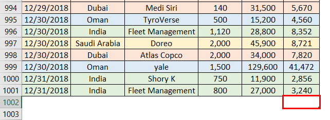
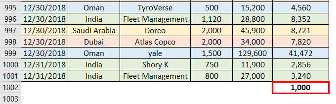
Suppose we have data of 1000 colored rows as shown below, and all we wanted is to find out the count of each color within the entire data. See the partial layout of the data given below:
Step 1: Go to cell F1002 to use the SUBTOTAL formula to capture the subtotal.
Step 2: Start typing the formula for SUBTOTAL inside the cell F1002. This formula has several function options within it. You can see the list as soon as the formula is active.
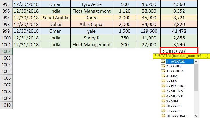
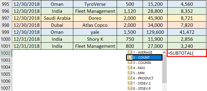
Step 3: Out of the list, you need to select function number 102 associated with the COUNT function. Use the mouse to drag towards function 102 and double click it to select.
Step 4: Use cells F1 to F10001 as a reference array within which the function COUNT will be used to count the cells. Fix the cell reference with the dollar sign, as shown in the screenshot below.
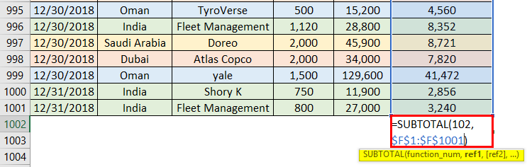
Step 5: Close the parentheses to complete the formula and press Enter key to see the output. You can see 1000 as a number in cell F1002.
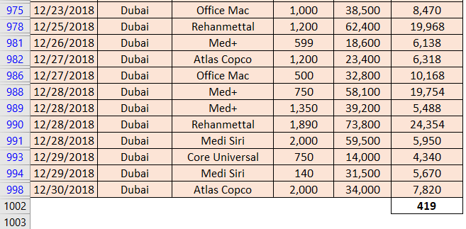
Step 6: Now apply a filter to the entire data and use the Filter by Cell Color option to filter the data with cell colors. As soon as you filter a specific color, the value of the cell F1002 will change to the number of cells that are with that specific color. See the screenshots below.
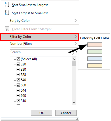
You can see there are 419 cells which have the same color as filtered, i.e. light orange. You similarly can check the count of other colors as well.
This works fine because of the use of the COUNT function (102) within the SUBTOTAL as an argument. The COUNT function counts all the non-empty cells within the given range, and subtotal gives the total of the counts. If we apply a filter with any specific criteria, due to the nature of SUBTOTAL, we only get the total count associated with those criteria (in this case, color).
Example #2 – Using COUNTIF and GET.CELL
We can also use the COUNTIF and a GET.CELL function in combination to get the count of colored cells. GET.CELL is an old macro function which does not work with most of the functions. However, it has compatibility with named ranges. This function can extract the extra piece of information which a normal CELL function could not extract. We use this function to get information about the color of a cell. Follow the steps to know how we can count the cells with color using these two functions.
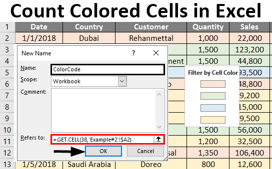
Step 1: Create a new named range ColorCode using the named ranges option within the Formulas tab.
Go to Formulas tab > inside Defined Names section, click on Define Name to be able to create a named range.
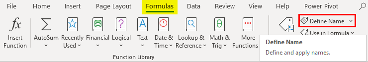
Step 2: A pop-up box with “New Name” will appear. Mention the name as ColorCode and within Refers to: section, use the formula as =GET.CELL(38,’Example #2′!$A2). Press OK after the amendments. Your named range will be completed and ready to use.
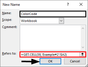
38 here is an operation number associated with GET.CELL. It is associated with an operation that captures the unique color numbers in Excel.
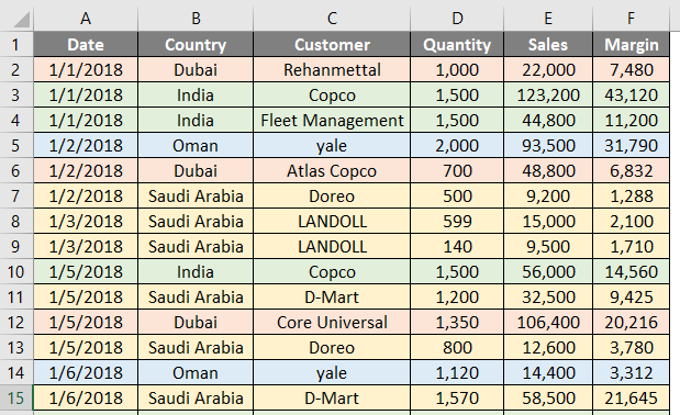
Rename column G as ColorCode, where we will capture the numeric codes associated with each color. These codes are unique for each color.
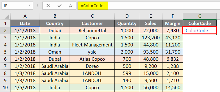
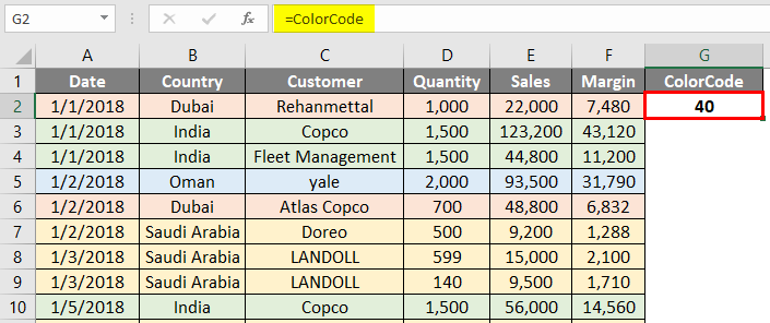
Step 3: In cell G2, start typing =ColorCode. This is the named range which we have just created in the previous step. Press Enter key to get a unique numeric code associated with the color of cell A2 (remember, while defining the named range, we used A2 as a reference from a sheet).
40 is the code associated with pink color in Excel.
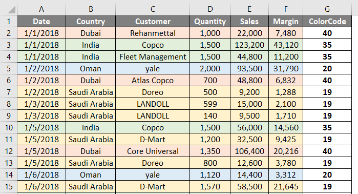
Step 4: Drag and paste the formula across cell G3:G1001, and you’ll see different numbers, which are nothing but the color codes associated with each color. See the partial screenshot below.
Step 5: Now, we need to calculate what is the count of each color in the sheet. For this, we will use the COUNTIF function. Start typing =COUNTIF in cell B1003 of the given excel sheet.
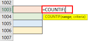
Please note that we have colored the cell 1003:1006 with the colors we have used respectively in our example.
Step 6: Use column G as a range argument to this function and ColorCode named range as a criterion. Complete the formula by closing the parentheses and see the output in cell B1003.
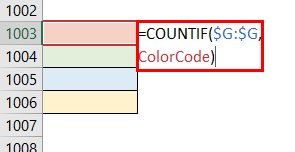
After using the formula, the output is shown below.
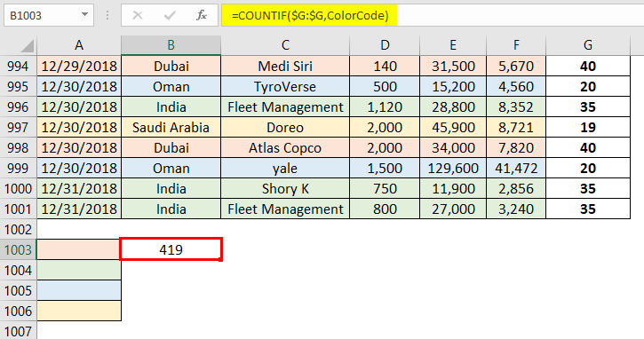
Drag and paste this formula across the remaining cells and see the count of remaining colors.
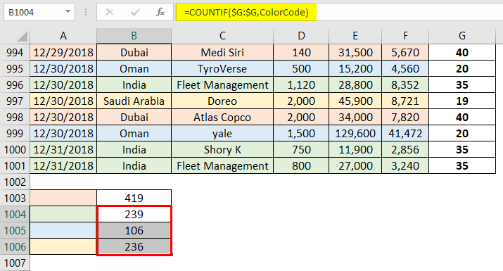
In this article, we have seen the different methods which can be used to find out the count of colored cells. Let’s wrap the things with some points to be remembered.
Things to Remember About Count Colored Cells In Excel
- We don’t have any built-in function which can count the colored cells in the excel sheet. However, we can use a different combination of formulae to capture the same.
- The CELL function, which we use in the second example, gives more information related to a cell that the general CELL function can’t provide.
- Numeric code 102 we use under the SUBTOTAL function is a numeric code of COUNT function under it.
Recommended Articles
This is a guide to Count Colored Cells in Excel. Here we discuss How to use Count Colored Cells in Excel along with practical examples and a downloadable excel template. You can also go through our other suggested articles –
- Count Cells with Text in Excel
- Count Characters in Excel
- COUNTIFS in Excel
- How to Add Cells in Excel
Top 3 Methods to Count Colored Cells In Excel
There is no built-in function to count colored cells in Excel, but below mentioned are three different methods to do this task.
- Count colored cells by using the Auto Filter option
- Count colored cells by using the VBA code
- Count colored cells by using the FIND method
Table of contents
- Top 3 Methods to Count Colored Cells In Excel
- #1 – Excel Count Colored Cells By Using Auto Filter Option
- #2 – Excel Count Colored Cells by using VBA Code
- #3 – Excel Count Colored Cells by Using FIND Method
- Things to Remember
- Recommended Articles
Now, let us discuss each of them in detail –
#1 – Excel Count Colored Cells By Using Auto Filter Option
For this example, let us look at the below data.
As we can see, each city is marked with different colors. So, we need to count the number of cities based on cell color.
As we can see, all the colors in the data. Now, we must choose the color that we want to filter.
We must follow the below steps to count cells by color.
- We must first apply the filter to the data.

- At the bottom of the data, we need to apply the SUBTOTAL function in Excel to count cells.

- The SUBTOTAL function contains many formulas. It is helpful if we want to count, sum, and average only visible cell data. Under the heading PIN, we must click on the drop-down list filter and select Choose by Color.

- As we can see, all the colors in the data. Now, we must choose the color that we want to filter.

Wow!!! As we can see in cell D21, our SUBTOTAL function is given the count of filtered cells as 6 instead of the previous result of 18.

Similarly, now we must choose other colors to get the count of the same.

So, blue-colored cells count to five now.
#2 – Excel Count Colored Cells by using VBA Code
VBA’s street smart techniques help us reduce time consumption at our workplace for some complicated issues.
We can reduce time, but we can also create our functions to fit our needs. For example, we can create a function to count cells based on color in one such function. Below is the VBA codeVBA code refers to a set of instructions written by the user in the Visual Basic Applications programming language on a Visual Basic Editor (VBE) to perform a specific task.read more to create a function to count cells based on color.
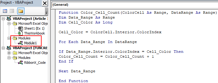
Code:
Function Color_Cell_Count(ColorCell As Range, DataRange As Range)

Dim Data_Range As Range
Dim Cell_Color As Long

Cell_Color = ColorCell.Interior.ColorIndex

For Each Data_Range In DataRange

If Data_Range.Interior.ColorIndex = Cell_Color Then
Color_Cell_Count = Color_Cell_Count + 1
End If

Next Data_Range

End Function
Then, copy and paste the above code to your module.
This code is not a SUB Procedure to run. Rather, it is a “User Defined FunctionUser Defined Function in VBA is a group of customized commands created to give out a certain result. It is a flexibility given to a user to design functions similar to those already provided in Excel.read more” (UDF).
The first line of the code “Color_Cell_Count” is the function name. Now, we must create three cells and color them as below.

Now, we must open the function “Color_Cell_Count” in the G2 cell.
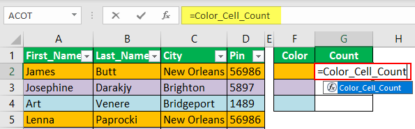
Even though we do not see the syntax of this function, the first argument is what color we need to count, so we must select cell F2.

The second argument is to select the range of cells as D2:D19.

Now, close the bracket and press the “Enter” key. As a result, it will provide the count of cells with the selected cell color.
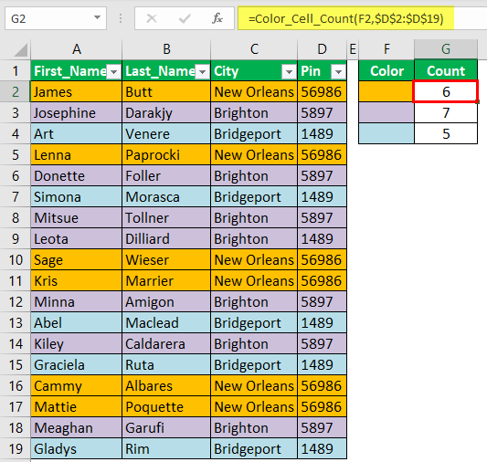
Like this, with the help of UDF in VBA, we can count cells based on cell color.
#3 – Excel Count Colored Cells by Using FIND Method
We can also count cells based on the FIND method as well.
- Step 1: First, we must select the range of cells where we need to count cells.

- Step 2: Now, we need to press Ctrl + F to open the FIND dialog box.

- Step 3: Now, click on “Options>>.”

- Step 4: Consequently, it will expand the “Find” dialog box. Now, we must click on the “Format” option.

- Step 5: Now, it will open up the “Find Format” dialog box. We need to click on the “Choose Format From Cell” option.

- Step 6: Now, move the mouse pointer to see the pointer to select the format cell in excelFormatting cells is an important technique to master because it makes any data presentable, crisp, and in the user’s preferred format. The formatting of the cell depends upon the nature of the data present.read more that we are looking to count.

- Step 7: We will select the cell formatted as the desired cell count. We have chosen the F2 cell as the desired cell format, and now we can see the preview.

- Step 8: Now, click on the “Find All” option to get the count of the selected cell format count of cells.

So, a total of 6 cells were found with selected formatting colors.
Things to Remember
- The provided VBA code is not a Subprocedure in VBASUB in VBA is a procedure which contains all the code which automatically gives the statement of end sub and the middle portion is used for coding. Sub statement can be both public and private and the name of the subprocedure is mandatory in VBA.read more; it is a UDF.
- The SUBTOTAL contains many formulas used to get the result only for visible cells when the filter is applied.
- We do not have any built-in function in Excel to count cells based on the color of the cell.
Recommended Articles
This article has been a guide to Count Colored Cells in Excel. We learned to count colored cells using the auto filter option, VBA code, FIND method, and downloadable Excel template. You may learn more about Excel from the following articles: –
- Shade Alternate Rows in Excel
- Countif not Blank in Excel
- Count Rows in Excel
- Word Count in Excel
The COUNT function in Excel counts cells containing numbers in Excel. You cannot count colored or highlighted cells with the COUNT function. But you can follow a few workarounds to count colored cells in Excel. In this tutorial, you will learn how to count colored cells in Excel.
In excel, you can count highlighted cells using the following workarounds:
- Applying SUBTOTAL and filtering the data
- Using the COUNT and GET.CELL function
- Using VBA
Using Subtotal and Filter functions
You can count highlighted cells in Excel by subtotaling the visible cells and applying a filter based on colors.
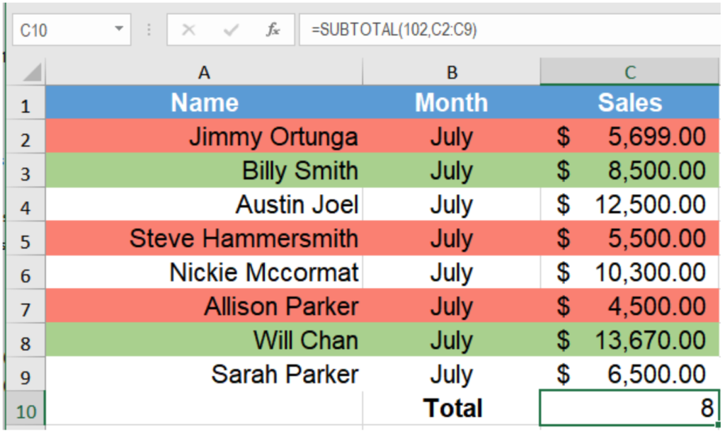
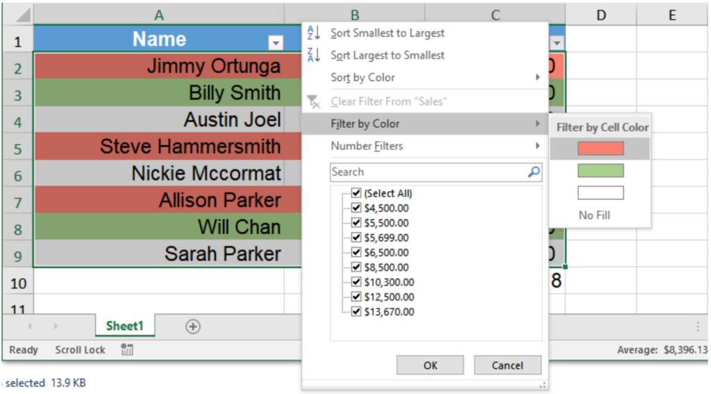
In this example, you have the sales record for eight salespersons for the month of July. The rows containing salespersons having sales less than $7000 is highlighted in red, the other cells with the salespersons having a bonus is highlighted in green. To calculate the number of salespersons highlighted in red:
- Select the cell C10.
- Assign the formula
=SUBTOTAL(102, C2:C9). The first argument 102 counts the visible cells in the specified range.
- Select cells A1:C9 by clicking on cell A1 and dragging it till C9 with your mouse.
- Go to Data > Sort & Filter > Filter.
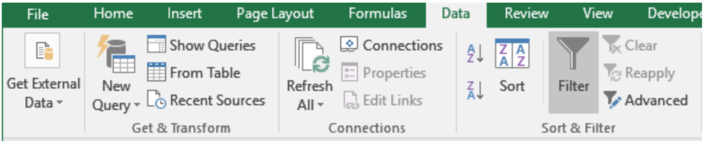
- Click on the filter drop downs in C1.
- Go to Filter by Color and select the color Red to find out the salespersons highlighted in red.
This will output change the subtotal value to x, which is the number of salespersons having sales less than $7000.
Using COUNTIF and GET.CELL functions
You can use GET.CELL with named ranges to count colored cells in Excel. GET.CELL is an old Macro4 function and does not work with regular functions. However, it still works with named ranges. To count colored cells with GET.CELL, you need to extract the color codes with GET.CELL and count them to find out the number of cells highlighted in the same color. To count cells using GET.CELL and COUNTIF:
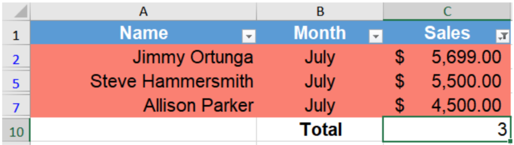
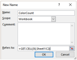
- Go to Formulas > Define Name.
- In the dialogue box that pops up, set name as ColorCount, scope as workbook and Refers to as
=GET.CELL(38, Sheet1!C2).
- Assign the formula =ColorCount to cell D2 and drag it till D9 with your mouse.
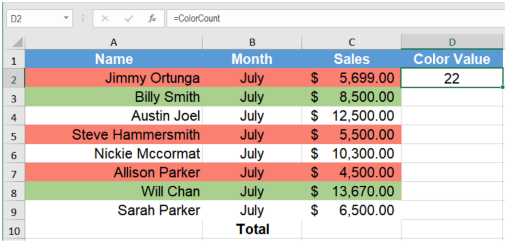
- This would return a number based on the background color. If there is no background color, Excel would return 0. Otherwise all cells with the same background color return the same number.
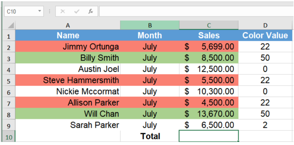
- From column D, look at the code for the color red. In this case it is 22.
- Select cell D10 and assign the formula
= COUNTIF($D:$D, 22).
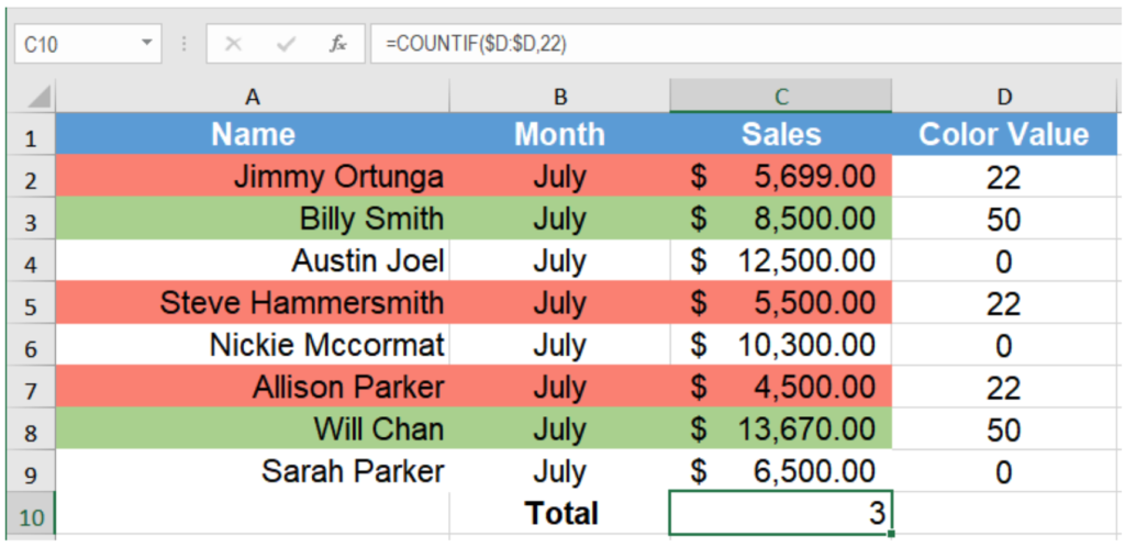
This will count the cells colored in red to find the number of salespersons with sales less than $7000 and return the number 3.
Using VBA
You can also create a custom function with VBA to count highlighted cells in Excel. To do that you need to create a custom function using VBA that works like a COUNTIF function and returns the number of cells for the same color.
You will follow the syntax: =CountFunction(CountColor, CountRange) and use it like other regular functions.Here CountColor is the color for which you want to count the cells. CountRange is the range in which you want to count the cells with the specified background color.
To count the cells highlighted in red, follow the steps below:
- Hold down the ALT + F11 keys, and it opens the Microsoft Visual Basic for Applications window.
- Click Insert > Module.
- Paste the following code in the Module Window.
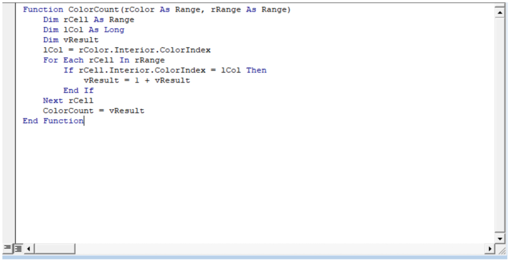
- In this code, you are defining a function with two arguments rColor and rRange. You are going to save the value of the background color of A2 in lCol. Then you are going to run a FOR loop where, if the cell’s background color matches the color in lCol, you increment vResult. This function returns the value of vResult, which is the count of the cells having the same background color.
- Then save the code, and apply the following formula to cell C10:
=ColorCount(A2, C2:C10).
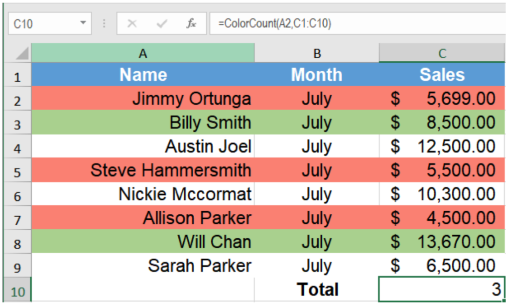
- Here A2 is the cell with the background color red you want to count. C2:C10 is the cell range that you want to count.
This will return the number of salespersons with sales less than $7000 in the month of July which is 3.