
Financial modeling in Excel refers to tools used for preparing the expected financial statements predicting the company’s financial performance in a future period using the assumptions and historical performance information. One may use such financial models in DCF valuations, mergers and acquisitions, private equity, project finance, etc.
Financial modeling in Excel is all around the web. There has been a lot written about learning financial modeling. However, most of the financial modeling pieces of training are the same. It goes beyond the usual gibberish and explores practical financial modeling used by Investment BankersInvestment banking is a specialized banking stream that facilitates the business entities, government and other organizations in generating capital through debts and equity, reorganization, mergers and acquisition, etc.read more and Research Analysts.
In this free financial modeling Excel guide, we will take the example of Colgate Palmolive (2016 – 2020) and prepare a fully integrated financial model from scratch.
This guide is over 5,000 words and took me three weeks to complete. Therefore, save this page for future reference, and do not forget to share it.
Financial Modeling in Excel Training – Read me First
Step 1 – Download the Colgate Financial Model Template.
You can download this Colgate Financial Modeling Templates (Solved/Unsolved) here – Colgate Financial Modeling Templates (Solved/Unsolved)
Step 2 – Please note you will get two templates – 1) Unsolved Colgate Palmolive Financial Model and 2) Solved Colgate Palmolive Financial Model.
Step 3- You will work on the Unsolved Colgate Palmolive Financial Model Template. Follow the step-by-step instructions to prepare a fully integrated financial model.
Step 4 – Happy Learning!
If you are new to financial modeling, look at this guide on What is Financial Modeling?Financial modeling refers to the use of excel-based models to reflect a company’s projected financial performance. Such models represent the financial situation by taking into account risks and future assumptions, which are critical for making significant decisions in the future, such as raising capital or valuing a business, and interpreting their impact.read more
How to Build a Financial Model in Excel?
Let us look at how one can build a financial model from scratch. This detailed financial modeling guide will provide a step-by-step guide to creating a financial model. The primary approach taken in this financial modeling guide is Modular. The modular system essentially means building core statements like income statements, balance sheets, and cash flows using different modules/sheets. The key focus is to prepare each statement step by step and connect all the supporting programs to the core statements on completion. We understand that this may not be clear now. However, you will realize this is very easy as we move forward.
- Step 1 – Colgate’s Financial Model – Historical
- Step 2 – Ratio Analysis of Colgate Palmolive
- Step 3 – Projecting the Income Statement
- Step 4- Working Capital Forecast
- Step 5 – Depreciation Forecast
- Step 6 – Amortization Forecast
- Step 7 – Other Long Term Forecast
- Step 8 – Completing the Income Statement
- Step 9 – Shareholder’s Equity Forecast
- Step 10 – Shares Outstanding Forecast
- Step 11 – Completing the Cash Flow Statements
- Step 12- Debt and Interest Forecast
Please note the following –
- The core statements are the Income StatementThe income statement is one of the company’s financial reports that summarizes all of the company’s revenues and expenses over time in order to determine the company’s profit or loss and measure its business activity over time based on user requirements.read more, Balance SheetA balance sheet is one of the financial statements of a company that presents the shareholders’ equity, liabilities, and assets of the company at a specific point in time. It is based on the accounting equation that states that the sum of the total liabilities and the owner’s capital equals the total assets of the company.read more, and Cash Flows.
- The different sheets are the depreciationDepreciation is a systematic allocation method used to account for the costs of any physical or tangible asset throughout its useful life. Its value indicates how much of an asset’s worth has been utilized. Depreciation enables companies to generate revenue from their assets while only charging a fraction of the cost of the asset in use each year.
read more forecast, working capital forecast, intangibles forecast, shareholder’s equityShareholder’s equity is the residual interest of the shareholders in the company and is calculated as the difference between Assets and Liabilities. The Shareholders’ Equity Statement on the balance sheet details the change in the value of shareholder’s equity from the beginning to the end of an accounting period.read more forecast, other long term items forecast, debt forecast scheduleA debt schedule is the list of debts that the business owes, including term loans, debentures, cash credit, etc. Business organizations prepare this schedule to know the exact amount of the company’s liability to others and manage its cash flows to prevent the financial crisis and enable better debt management.read more, etc. - The different schedules are linked to the core statements upon their completion.
- This financial modeling guide will build a step-by-step integrated economic model of Colgate Palmolive from scratch.
Step 1 – Financial Modeling in Excel – Project the Historicals
The first step in the financial modeling guide is to prepare the historicals.
Download Colgate’s 10K Reports
One prepares financial models in Excel. The first steps start with knowing how the industry has been doing recently. Understanding the past can provide valuable insights into the company’s future. Therefore the first step is to download all the company’s financials and populate the same in an Excel sheet. For Colgate Palmolive, you can download the annual reports of Colgate Palmolive from their Investor Relation Section.
Create the Historical Financial Statements Worksheet
- If you download 10K of 2020, you will note that only two years of financial statement data is available. However, for financial modeling in Excel, the recommended dataset is to have the last 5 years of financial statements. Therefore, please download the last 3 years of the annual reportAn annual report is a document that a corporation publishes for its internal and external stakeholders to describe the company’s performance, financial information, and disclosures related to its operations. Over time, these reports have become legal and regulatory requirements.read more and populate the historical.
- Often, these tasks seem too tedious as it may take a lot of time and energy to format and put the excel in the desired format.
- However, one should not forget that this is the work you are required to do only once for each company. Populating the historicals also helps an analyst understand the trends and financial statementsFinancial statements are written reports prepared by a company’s management to present the company’s financial affairs over a given period (quarter, six monthly or yearly). These statements, which include the Balance Sheet, Income Statement, Cash Flows, and Shareholders Equity Statement, must be prepared in accordance with prescribed and standardized accounting standards to ensure uniformity in reporting at all levels.read more.
- So, please do not skip this. Instead, download and populate the data (even if you feel this is the donkey’s work).
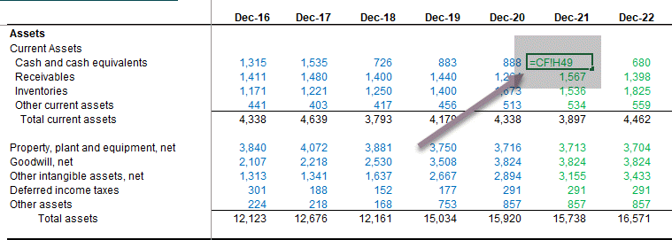
Colgate Income Statement with Historical Populated
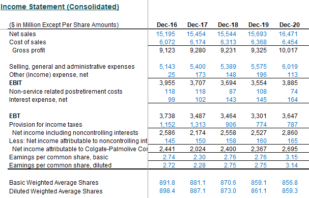
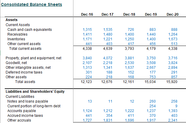
Colgate Balance Sheet Historical Data
Step 2 – Ratio Analysis
The second step in financial modeling in Excel is to perform ratio analysis. We covered this in detail in part 1 of the series – Ratio AnalysisRatio analysis is the quantitative interpretation of the company’s financial performance. It provides valuable information about the organization’s profitability, solvency, operational efficiency and liquidity positions as represented by the financial statements.read more
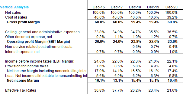
Vertical Analysis of Colgate
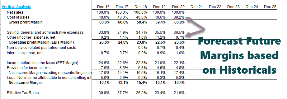
On the income statement, the vertical analysis is a universal tool for measuring the firm’s relative performance from year to year in terms of cost and profitability. Therefore, it should always be included as part of any financial analysis. Here, percentages are computed concerning net sales, which is considered 100%. This vertical analysis effort in the income statement is often referred to as margin analysis since it yields different margins concerning sales.
Horizontal Analysis of Colgate
Horizontal analysis is a technique used to evaluate trends over time by calculating percentage increases excelPercentage increase = (New Value — Old Value)/ Old Value. Instead of showing the delta as a Value, percentage increase shows how much the value has changed in terms of percentage increase.read more or decreases relative to a base year. It provides an analytical link between accounts calculated at different dates using the currency with varying purchasing powers. In effect, this analysis indexes the reports and compares these evolved. As with the vertical analysisVertical analysis is a kind of financial statement analysis wherein each item in the financial statement is shown in percentage of the base figure. The formula is: (Statement line item / Total base figure) X 100read more methodology, issues that need to be investigated and complemented with other financial analysis techniques will surface. The focus is to look for symptoms of problems that one can diagnose using additional methods.
Let us look at the horizontal analysis of Colgate.

Liquidity Ratios of Colgate
- Liquidity ratios measure the relationship of the more liquid assetsLiquid Assets are the business assets that can be converted into cash within a short period, such as cash, marketable securities, and money market instruments. They are recorded on the asset side of the company’s balance sheet.read more of an enterprise (the ones most easily convertible to cash) to current liabilities. The most common liquidity ratios are the current ratioThe current ratio is a liquidity ratio that measures how efficiently a company can repay it’ short-term loans within a year. Current ratio = current assets/current liabilities
read more, Acid test (or quick asset) ratio Cash RatiosCash Ratio is calculated by dividing the total cash and the cash equivalents of the company by total current liabilities. It indicates how quickly a business can pay off its short term liabilities using the non-current assets.read more. - Turnover Ratios like Accounts ReceivablesAccounts receivables is the money owed to a business by clients for which the business has given services or delivered a product but has not yet collected payment. They are categorized as current assets on the balance sheet as the payments expected within a year.
read more turnover, inventory turnover, and payables turnover.
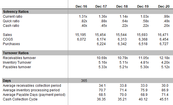
Also, have a look at this detailed article on Cash Conversion CycleThe Cash Conversion Cycle (CCC) is a ratio analysis measure to evaluate the number of days or time a company converts its inventory and other inputs into cash. It considers the days inventory outstanding, days sales outstanding and days payable outstanding for computation.read more.
Operating Profitability Ratios of Colgate
Profitability ratiosProfitability ratios help in evaluating the ability of a company to generate income against the expenses. These ratios represent the financial viability of the company in various terms.read more are a company’s ability to generate earnings relative to sales, assets, and equity.
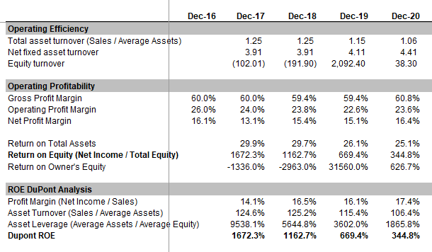
Risk Analysis of Colgate
Through Risk AnalysisRisk analysis refers to the process of identifying, measuring, and mitigating the uncertainties involved in a project, investment, or business. There are two types of risk analysis — quantitative and qualitative risk analysis.read more, we try to gauge whether the companies will be able to pay their short and long-term obligations (debt). We calculate leverage ratiosDebt-to-equity, debt-to-capital, debt-to-assets, and debt-to-EBITDA are examples of leverage ratios that are used to determine how much debt a company has taken out against its assets or equity.read more that focus on the sufficiency of assets or generation from assets. Rates that looks at are:
- Debt to Equity Ratio
- Debt ratio
- Interest Coverage RatioThe interest coverage ratio indicates how many times a company’s current earnings before interest and taxes can be used to pay interest on its outstanding debt. It can be used to determine a company’s liquidity position by evaluating how easily it can pay interest on its outstanding debt.read more

Step 3 – Financial Modeling in Excel – Project the Income Statement
The third step in financial modeling is to forecast the income statement, wherein we will start with modeling the sales or revenue items.
Revenues Projections
For most companies, revenues are a fundamental driver of economic performance. Therefore, a well-designed and logical revenue model reflecting the type and amounts of income flows accurately is extremely important. There are as many ways to create a revenue schedule as there are businesses. Some common types include:
- Sales Growth: Sales growth assumption in each period defines the change from the previous period. It is a simple and commonly used method but offers no insights into the components or dynamics of growth.
- Inflationary and Volume/ Mix effects: Instead of a simple growth assumption, a price inflation factor and a volume factor are used. This useful approach allows the modeling of fixed and variable costs in multi-product companies and considers price vs. volume movements.
- Unit Volume, Change in Volume, Average Price, and Change in Price: This method is appropriate for businesses with a simple product mix. It permits analysis of the impact of several key variables.
- Dollar Market Size and Growth: Market share and change in share – useful for cases where information is available on market dynamicsMarket Dynamics is defined as the forces of market constituents responsible for the shift in the demand and supply curve and are therefore accountable for creating and reducing the demand and supply of a particular product.read more and where these assumptions are likely to be fundamental to a decision. For example, the telecom industry.
- Unit Market Size and Growth: This is more detailed than the preceding case and is useful when pricing in the market is a crucial variable. (For a company with a price-discounting strategy. For example, a best-of-breed premium-priced niche player) e.g., the luxury car market
- Volume Capacity, Capacity Utilization Rate, and Average Price: These assumptions can be important for businesses where production capacity is essential to the decision. (In purchasing additional capacity, for example, or determining whether the expansion would require new investments).
- Product Availability and Pricing
- Revenue was driven by investment in capital, marketing, or R&D
- Revenue-based on installed base (continuing sales of parts, disposables, services, add-ons, etc.). Examples include classic razor-blade businesses and businesses like computers where sales of service, software, and upgrades are essential. Again, modeling the installed base is key (new additions to the floor, attrition in the ground, continuing revenues per customer, etc.).
- Employee based: For example, revenues of professional services firms or sales-based firms such as brokers. Modeling should focus on net staffing and revenue per employeeRevenue Per Employee is the ratio of total revenue over total number of employees in a particular accounting period. It gives an idea about how the business performed.read more (often based on billable hours). More detailed models will include seniority and other factors affecting pricing.
- Store, facility, or Square footage based: Retail companies are often modeled based on stores (old stores plus new stores each year) and revenue per store.
- Occupancy-factor-based: This approach applies to airlines, hotels, movie theatres, and other businesses with low marginal costs.
Projecting Colgate Revenues
Let us now look at the Colgate 10K 2020 report. First, Colgate has not provided segmental information in the income statement. However, as additional information, Colgate has provided details of each segment.
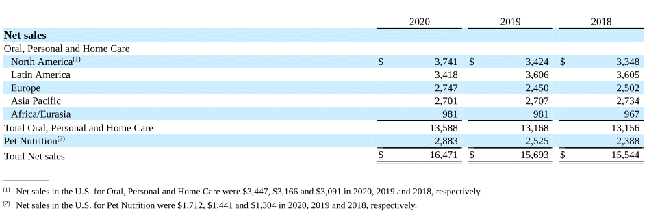
Source – Colgate 2020 – 10K, Page 119
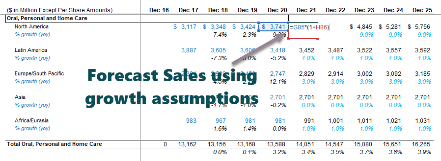
Since we do not have any further information about the features, we will project the future sales of Colgate based on this available data. We will use the sales growth approach across segments to derive the forecasts. Please see the picture below. We have calculated the year-over-year growth rate for each element.

Now, we can assume a sales growth percentage based on the historical trends and project the revenues under each part. Therefore, total net sales are the total of the Oral, Personal & Home Care, and Pet Nutrition Segment.
Costs Projections
- Percentage of Revenues: Simple but offers no insight into any leverage (economy of scale or fixed cost burden.
- Costs other than depreciation as a percent of revenues and depreciation from a different schedule: This approach is the minimum acceptable in most cases and permits only partial analysis of operating leverageOperating Leverage is an accounting metric that helps the analyst in analyzing how a company’s operations are related to the company’s revenues. The ratio gives details about how much of a revenue increase will the company have with a specific percentage of sales increase – which puts the predictability of sales into the forefront.read more.
- Variable costs based on revenue or volume, fixed costs based on historical trends, and depreciation from a different schedule. This approach is the minimum necessary for sensitivity analysisSensitivity analysis is a type of analysis that is based on what-if analysis, which examines how independent factors influence the dependent aspect and predicts the outcome when an analysis is performed under certain conditions.read more of profitability based on multiple revenue scenarios.
Cost Projections for Colgate
For projecting the cost, the vertical analysis done earlier will be helpful. So, let us have a relook at the vertical analysis:
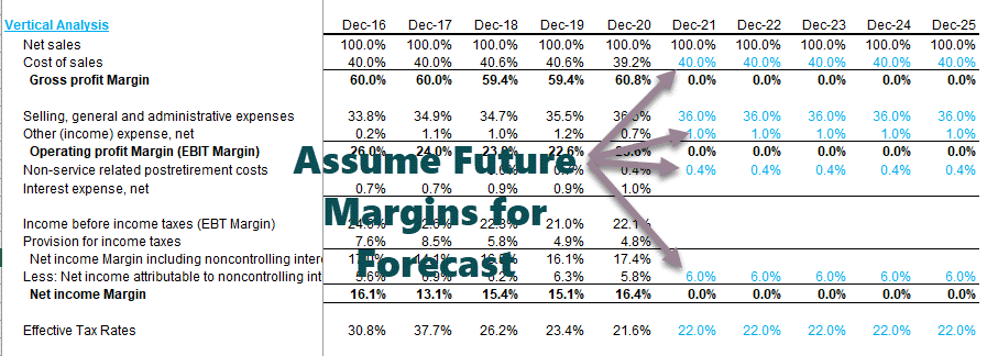
- Since we have already forecasted sales, all the other costs are some margins of these sales.
- The approach is to take the guidelines from the historical cost and expense margins and then forecast the future margin.
- For example, the cost of sales has been in the range of 39.2%-40.6% for the past five years. So we can look at forecasting the margins on this basis.
- Likewise, selling, general, and Administrative ExpensesSelling, general and administrative (SG&A) expense includes all the expenses incurred in the selling of the products of the company whether direct or indirect along with the entire general and the administrative expenses during an accounting period under consideration such as advertisement expenses, sales promotion expenses, marketing salaries, etc.read more have been historically in the range of 33.8%-36.5%. We can assume the future SG&A expense margin on this basis. Likewise, we can go on for another set of expenses.
Using the above margins, we can find the actual values by back calculations.
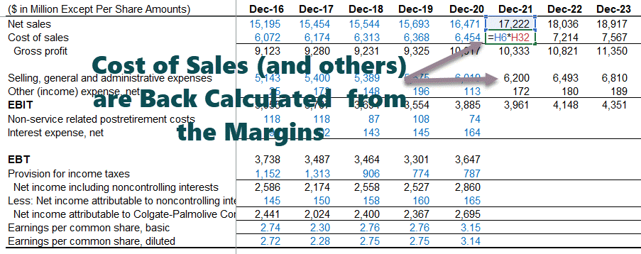
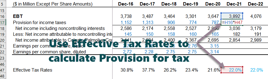
We use the effective tax rate assumption to calculate the provision for taxes.
- Also, note that we do not complete the “Interest Expense (Income)” row as we will look at the income statement later.
- Interest Expense and Interest Income.Interest Income is the amount of revenue generated by interest-yielding investments like certificates of deposit, savings accounts, or other investments & it is reported in the Company’s income statement. read more
- We have also not calculated depreciation and amortization, which we have already included in the cost of sales.
- This completes the income statement (at least for the time being!).
Step 4- Financial Modeling – Working Capital Schedule
Now that we have completed the income statement, the fourth step in financial modeling is to look at the working capital schedule.
Below are the steps that one must follow for a working capital schedule.
Link the Net Sales and Cost of Sales
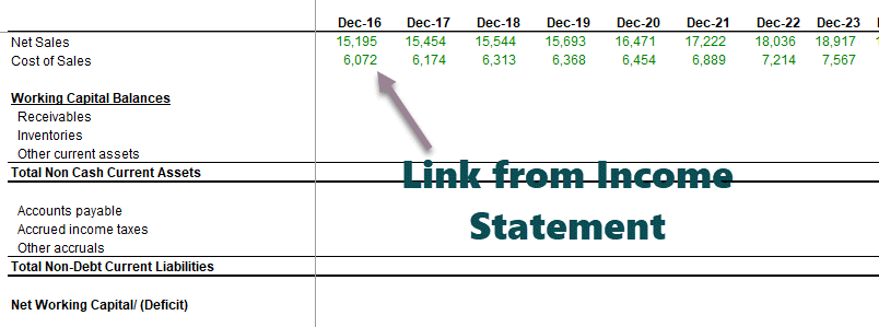
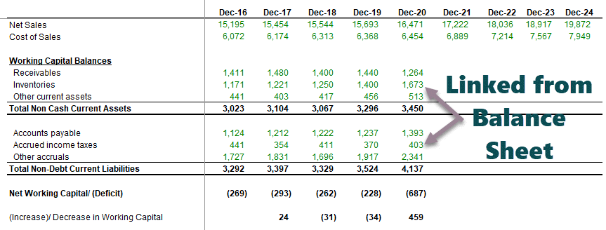
- Reference the past data from the balance sheet.
- Calculate net working capitalThe change in net working capital of a firm from one accounting period to the next is referred to as the change in net working capital. It is calculated to ensure that the firm maintains sufficient working capital in each accounting period so that there is no shortage of funds or that funds do not sit idle in the future.read more
- Arrive at an increase/ decrease in working capital
- Note that we have not included short-term debt and cash and cash equivalents in the working capital. We will deal with debt and cash and cash equivalentsCash and Cash Equivalents are assets that are short-term and highly liquid investments that can be readily converted into cash and have a low risk of price fluctuation. Cash and paper money, US Treasury bills, undeposited receipts, and Money Market funds are its examples. They are normally found as a line item on the top of the balance sheet asset. read more separately.
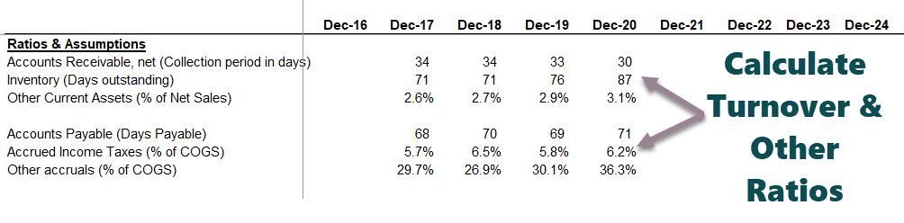
Calculate the Turnover Ratios
- Calculate historical ratios and percentages
- Use the ending or average balance.
- Both are acceptable as long as consistency is maintained.
Populate the assumptions for future working capital items
- Certain items without a prominent driver are assumed usually at constant amounts.
- Ensure assumptions are reasonable and in line with the business.

Project the future working capital balances
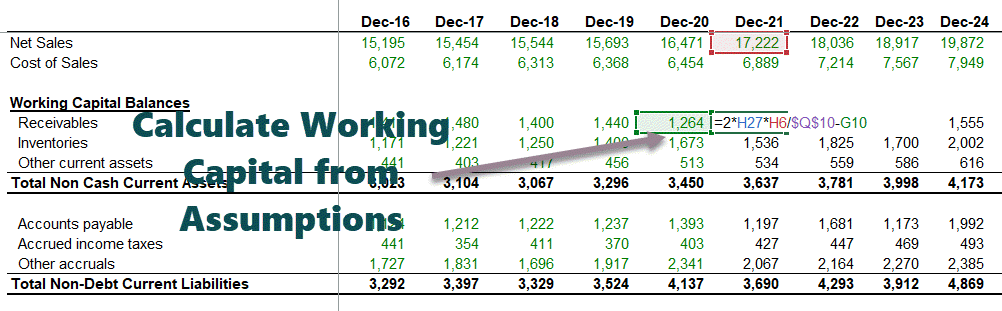
Calculate the changes in Working Capital
- Arrive at cash flows based on individual line items.
- Ensure signs are accurate!
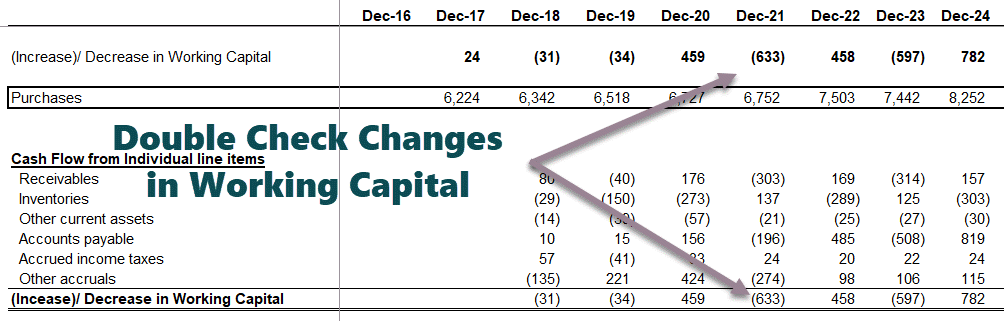
Link up the Working Capital Forecasts to the Balance Sheet
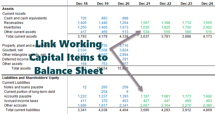
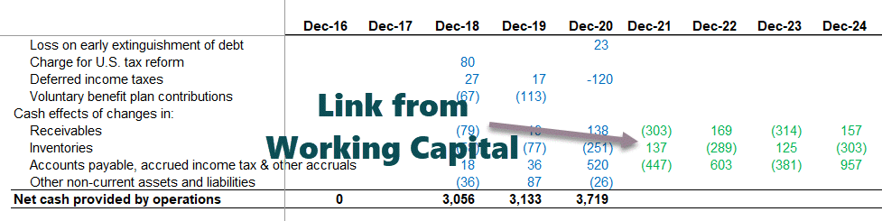
Link Working Capital Items to the Cash Flow Statement 
Step 5 – Financial Modeling in Excel – Depreciation Schedule
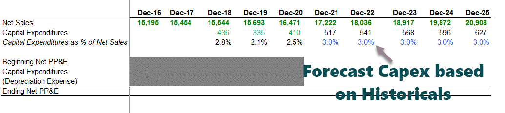
With the completion of the working capital schedule, the next step in this financial modeling is to project the CapexCapex or Capital Expenditure is the expense of the company’s total purchases of assets during a given period determined by adding the net increase in factory, property, equipment, and depreciation expense during a fiscal year.read more of Colgate and the depreciation and assets figures.

source – Colgate 10K 2020 Page – 72
- It has not provided depreciation and amortization as separate line items. However, it is included in the cost of sales.
- In such cases, please look at the cash flow statements, where you will find the depreciation and amortization expense. Also, note that the below figures are 1) Depreciation and 2) amortization. So, what is the depreciation number?
- Ending Balance for PPE = Beginning balance + Capex – Depreciation – Adjustment for Asset Sales (BASE equation).

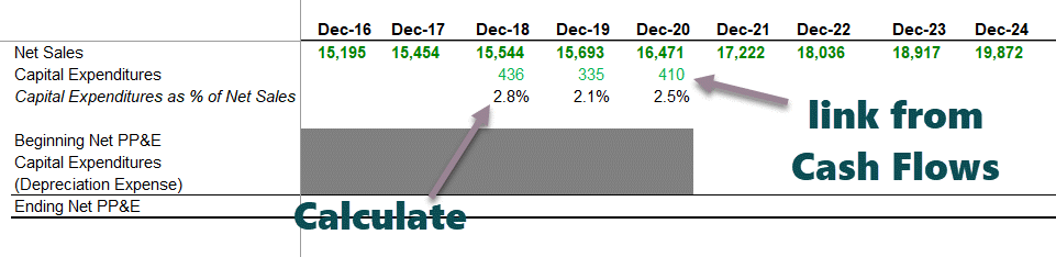
Link the Net Sales figures in the Depreciation Schedule
- Set up the line items
- Reference net sales
- Input past capital expenditures
- Arrive at Capex as a % of net sales
Forecast the Capital Expenditure Items
- There are various approaches to forecasting capital expenditure. One common practice is to look at the press releases, management projections, and MD&A to understand the company’s view on future capital expenditure.
- If the company has guided future capital expenditure, we can take those numbers directly.
- However, if the Capex numbers are not directly available, we can calculate it crudely using Capex as % of Sales (as done below).
- Use your judgment based on industry knowledge and other reasonable drivers.
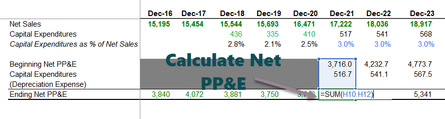
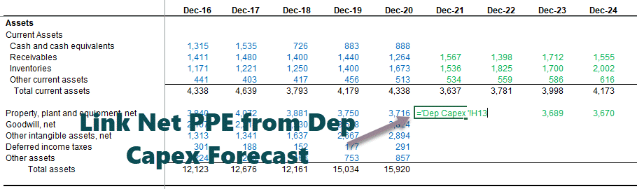
Reference Past Information and Calculate Net PP&E
- We will use Ending Balance for PPE = Beginning balance + Capex – Depreciation – Adjustment for Asset Sales (BASE equation)
- It is complicated to reconcile past PP&E due to restatementsA restatement is the revision of already issued financial statements of one or more companies to correct errors with material inaccuracy due to non adhering and complying with the GAAP, accounting mistakes, fraud, or clerical errors affecting part of the entire financial statement requiring a completely new audit.read more, asset sales, etc.
- It is therefore recommended not to reconcile the past PPE as it may lead to some confusion.
Depreciation Policy of Colgate
- Colgate has not explicitly provided a detailed breakup of the Assets. Instead, they clubbed all assets into the land, building, machinery, and other equipment.
- Also, useful lives for machinery and equipment are provided in range. In this case, we will have to do some guesswork to determine the average useful life left for the assets.
- Also, guidance for useful life is not provided for “Other equipment.” Therefore, we will have to estimate the useful life of other equipment.
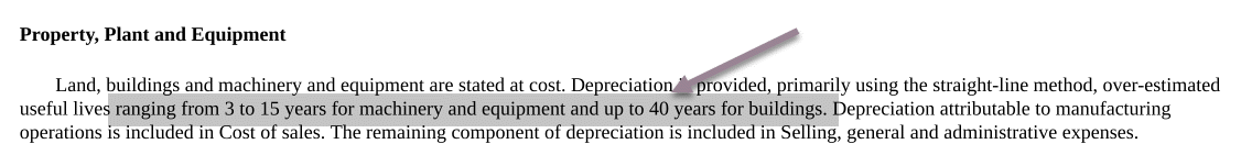
Colgate 2020 – 10K, Page 79
Below is the breakup of 2012 and 2013 Property, Plant, and Equipment Details
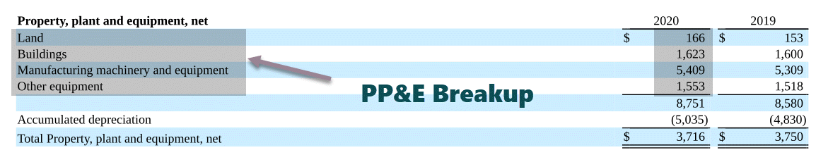
Colgate 2020 – 10K, Page 125
Estimate the breakup of Property Plant and Equipment (PPE)
- First, find the Asset weights of the Current PPE (2020)
- We will assume that these asset weights of 2020 PPE will continue going forward.
- We use these asset weights to calculate the breakup of estimated capital expenditure.
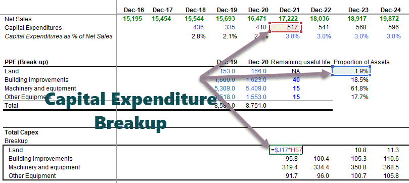
Estimate the Depreciation of Assets
- Please note that we do not calculate depreciation of LandThe land is a company asset with an infinite useful life. As a result, it is not subject to depreciation, unlike other long-term assets such as buildings and furniture, which have a limited useful life and thus require their costs to be allocated to the accounting period.read more as land is not a depreciable asset.
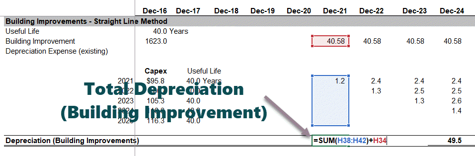
- For estimating depreciation from Building improvements, we first make use of the below structure.
- Depreciation here is divided into two parts: 1)Depreciation from the building improvements asset already listed on the balance sheet, 2) depreciation from the future Building improvements.
- We use the simple Straight Line Method of depreciationStraight Line Depreciation Method is one of the most popular methods of depreciation where the asset uniformly depreciates over its useful life and the cost of the asset is evenly spread over its useful and functional life. read more to calculate the depreciation from building improvements listed on the asset.
- For calculating future depreciation, we first transpose the Capex using the TRANSPOSE Function in ExcelThe TRANSPOSE function in excel helps rotate (switch) the values from rows to columns and vice versa. Being a part of the Excel lookup and reference functions, its purpose is to organize the data in the desired format. To execute the formula, the exact size of the range to be transposed is selected and the CSE key (“Control+Shift+Enter”) is pressed.
read more. - We calculate the depreciation from asset contributions from each year.
- Also, the first-year depreciation is divided by two as we assume the mid-year convention for asset deployment.

Total Depreciation of BuildingDepreciation of building refers to reducing the recorded cost of a building until the value of the structure either becomes zero or reaches its salvage value. In addition, it helps to map the revenue in the form of lease rental generated during the corresponding expenses.read more improvement = depreciation from the asset already listed on the balance sheet + depreciation from the future building improvements.
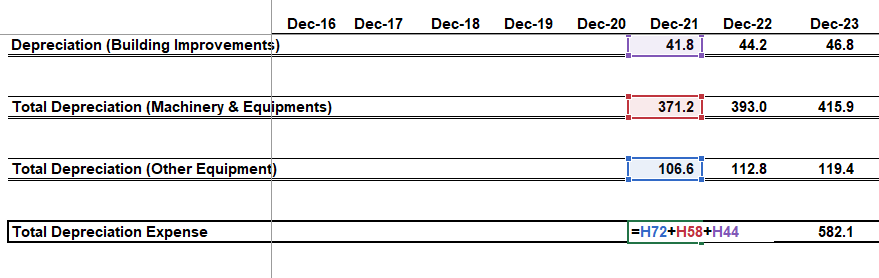
In the above process for estimating depreciation, one may calculate the depreciation of 1) manufacturing equipment & machinery and 2) other equipment, as shown below.
Total Depreciation of Colgate = Depreciation (Building Improvements) + Depreciation (Machinery & Equipment) + Depreciation (additional equipment)
Once we have found the real depreciation figures, we can put that in the BASE equation as shown below.
- With this, we get the ending net PP&E figures for each year.
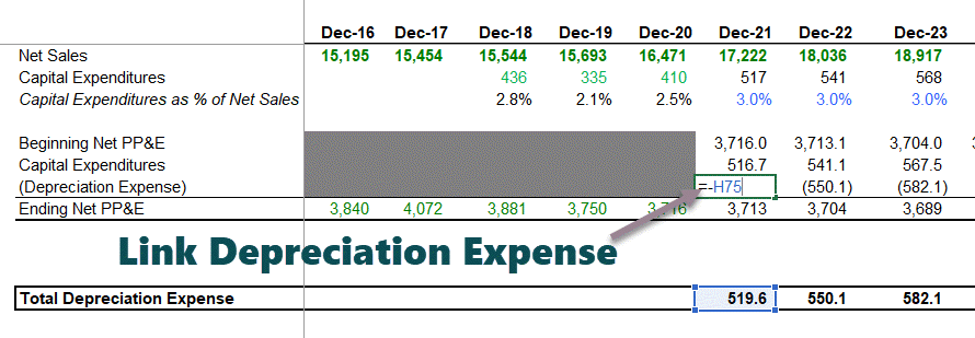
Link the Net PP&E to the Balance Sheet
Step 6 – Amortization Schedule
The sixth step in this financial modeling in Excel is to forecast the amortization. Again, we have two broad categories to consider here – 1) GoodwillIn accounting, goodwill is an intangible asset that is generated when one company purchases another company for a price that is greater than the sum of the company’s net identifiable assets at the time of acquisition. It is determined by subtracting the fair value of the company’s net identifiable assets from the total purchase price.read more and 2) Other Intangibles.
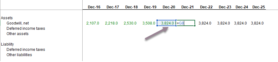
Forecasting Goodwill
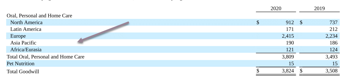
Colgate 2020 – 10K, Page 88
- Goodwill comes on the balance sheet when a company acquires another company. It usually is complicated to project goodwill for future years.
- However, Goodwill is subject to impairment tests annually, which the company performs. Therefore, analysts are in no position to conduct such tests and prepare estimates of impairments.
- Most analysts do not project goodwill. They just keep this constant, which we will do in our case.
Forecasting Other Intangible Assets
- Colgate’s 10K Report notes that most of the finite life intangible is related to the Sanex acquisition.
- “Additions to Intangibles” are also complicated to project.
- Colgate’s 10K report provides us with the details of the next five years of amortization expenses.
- We will use these estimates in our financial model.
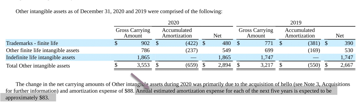
Colgate 2020 – 10K, Page 88
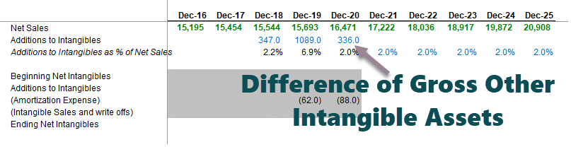
Calculate Ending Net Intangibles
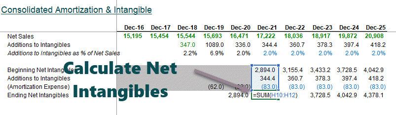
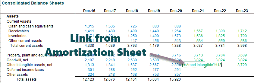
Ending net intangibles are linked to the “Other Intangible Assets.”
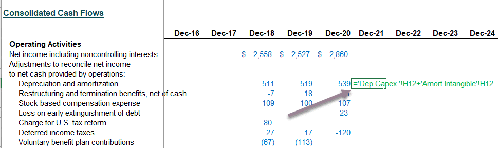
Link Depreciation and Amortization to Cash Flow Statements
Link Capex & Addition to Intangibles to Cash flow statements
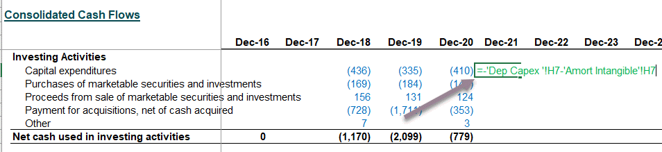
Step 7 – Other Long Term Schedule
The next step in this financial modeling is to prepare the other long-term schedule. It is when we prepare for the “leftovers” that do not have specific drivers for forecasting. In the case of Colgate, the other long-term items (leftovers) were Deferred Income TaxesDeferred income tax is a balance sheet item that can be either a liability or an asset since it is a difference in income recognition between the firm’s accounting records and the tax law, resulting in the company’s income tax due being different than the total tax expense reported.read more (liability and assets), other investments, and other liabilities.
Reference the historical data from the Balance Sheet
Also, calculate the changes in these items.
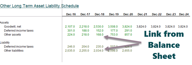
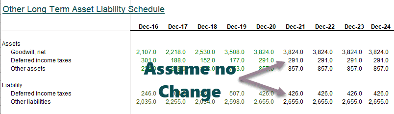
Forecast the Long Term Assets and Liabilities
- Keep the long-term items constant for projected years in case of no visible drivers.
- Link the forecasted long term items to the Balance SheetAssets such as cash, inventories, accounts receivable, investments, prepaid expenses, and fixed assets; liabilities such as long-term debt, short-term debt, Accounts payable, and so on are all included in the balance sheet.read more as shown below.
Reference Other Long Term Items to the Balance Sheet

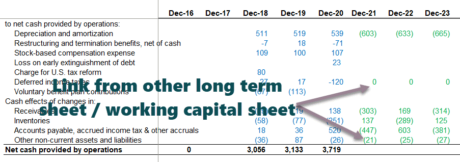
Link the long term items to the Cash Flow Statement
Please note that if we keep the long-term assets and liabilities constant, the change that flows to the cash flow statement would be zero.
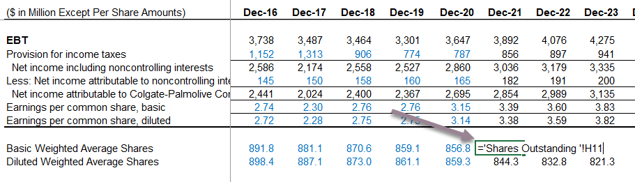
Step 8 – Financial Modeling in Excel – Completing the Income Statement
- Before we move any further in this Excel-based financial modeling, we will review the income statement.
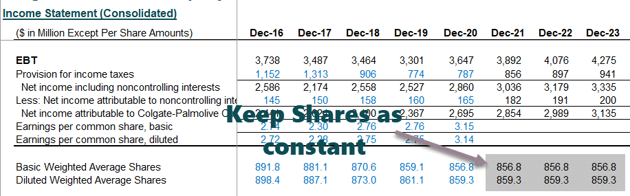
- Populate the historical basic weighted average shares and dilute the weighted average number of shares
- These figures are available in Colgate’s 10K report.
Reference the basic and diluted shares
At this stage, assume that the future number of primary and diluted shares will remain the same as in 2020.
We are ready to move to our next shareholder’s equity schedule.

Step 9 – Financial Modelling – Shareholder’s Equity Schedule
The next step in this financial modeling in Excel training is to look at the shareholder’s equity schedule. The primary objective of this schedule is to project equity-related items like shareholder’s equity, dividends, Share buybackShare buyback refers to the repurchase of the company’s own outstanding shares from the open market using the accumulated funds of the company to decrease the outstanding shares in the company’s balance sheet. This is done either to increase the value of the existing shares or to prevent various shareholders from controlling the company.read more, option proceeds, etc.
Colgate’s 10K report provides us with the details of common and treasury stock activities in the past years, as shown below.
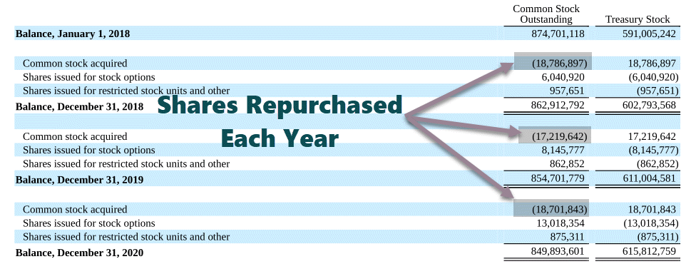
Colgate 10K 2020 – Page 97
- Historically, Colgate has repurchased shares, as shown in the schedule above.
- Populate Colgate’s shares repurchase (millions) in the Excel sheet.
- Link the historical diluted EPS from the income statement.
- The historical amount repurchased should be referenced from the cash flow statementsA Statement of Cash Flow is an accounting document that tracks the incoming and outgoing cash and cash equivalents from a business.read more.
Also, have a look at Accelerated Share RepurchaseAccelerated share repurchase (buyback) is a strategy adopted by a publicly-traded company to acquire its outstanding shares in the market from the clients in large blocks via an investment bank.read more.
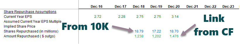
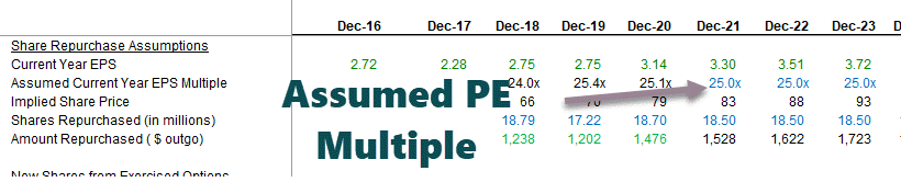
- Calculate the implied average price at which Colgate has done share repurchases historically. One may calculate the Amount repurchased / Number of shares.
- Calculate the PE multipleThe price to earnings (PE) ratio measures the relative value of the corporate stocks, i.e., whether it is undervalued or overvalued. It is calculated as the proportion of the current price per share to the earnings per share. read more = Implied Share Price / EPS

Colgate has not officially announced how many shares they intend to buy back. The only information that their 10K report shares are that they have authorized a buyback of up to 50 million shares.

Colgate 10K 2020 – Page 97
- We need to assume the share repurchase amount to find the number of shares repurchased. Based on the historical repurchase amount, we have taken this number as $1,500 million for all the future years.
- We need the projected implied share price of the potential buyback to find the number of shares repurchased.
- Actual share price = assumed PE multiplex EPS.
- One can assume future buyback PE multiple based on historical trends. We note that Colgate has repurchased shares at an average PE range of 17x – 25x.
- Below is the snapshot from Reuters that helps us validate the PE range for Colgate.

- In our case, we have assumed that all future buybacks of Colgate will be at a PE multiple of 25x.
- Using the PE of 25x, we can find the implied price = EPS x 25.
- Now that we have found the implied price, we can see the number of shares repurchased = $ amount used for repurchase / implied price.
Stock Options: Populate Historical Data
- The common stock and shareholder’s equity summary shows us the number of options exercises each year.
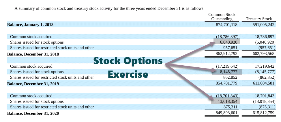
Colgate 2020 – 10K, Page 97
- Besides, we also have the option proceeds from the cash flow statements (approx).
- With this, we should be able to find an effective strike priceExercise price or strike price refers to the price at which the underlying stock is purchased or sold by the persons trading in the options of calls & puts available in the derivative trading. Thus, the exercise price is a term used in the derivative market.read more.
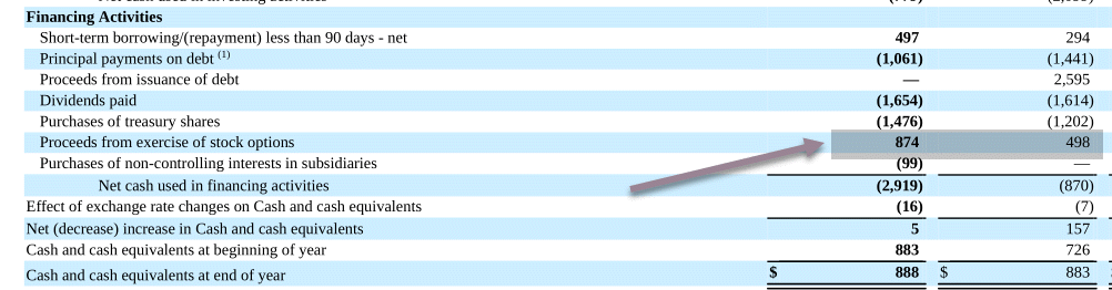
Colgate 2020 – 10K, Page 76
Also, note that the stock optionsStock options are derivative instruments that give the holder the right to buy or sell any stock at a predetermined price regardless of the prevailing market prices. It typically consists of four components: the strike price, the expiry date, the lot size, and the share premium.read more have contractual terms of eight years and vest over three years.

Colgate 2020 – 10K, Page 100
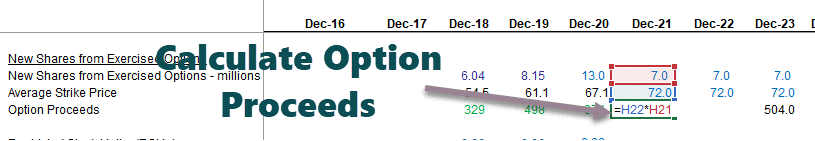
With this data, we fill up the options data as per below. We also note that the weighted average strike price of stock options for 2020 was $72, and the number of options outstanding was 27.541 million.
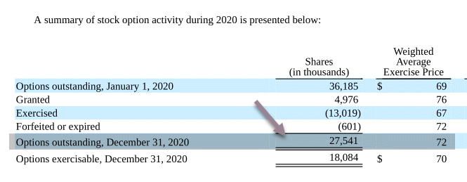
Colgate 2020 – 10K, Page 100
Stock Options: Find the Option Proceeds.
Our options data below shows that the option proceeds were $504 million in 2021. We have assumed that 7 million options exercise each year.
Stock Options: Forecast Restricted Stock Unit Data
In addition to the stock options, there are Restricted Stock UnitsRestricted Stock Units or RSU can be defined as stock-based compensation that is issued as company’s stock to an employee. The company establishes vesting requirements based on the performance of an individual and the length of the employment.read more are given to the employees and awarded and vested at the end of each three-year performance period.

Colgate 2020 – 10K, Page 99
Populating this data in the restricted stock units dataset.
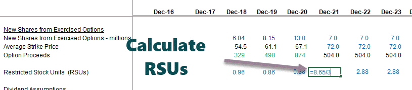
The restricted stock units project to be (8.65/3.0 years), i.e., 2.88 million going forward.
Also, have a look at the Treasury Stock MethodTreasury Stock Method is an accounting approach assuming that the options & stock warrants are exercised at the beginning of the year (or date of issue, if later) & proceeds from the exercise of these options & warrants are used to repurchase shares in the market. read more.
Dividends: Forecast the Dividends
- Forecast estimated dividends using the Dividend Payout Ratio.
- Fixed dividend outgo per-share payout.
- From the 10K reports, we extract all past information on dividends.
- With the information on dividends paid, we can find the Dividend Payout Ratio = Total Dividends Paid / Net Income.
- We have calculated the dividends payout ratio of Colgate as seen below:
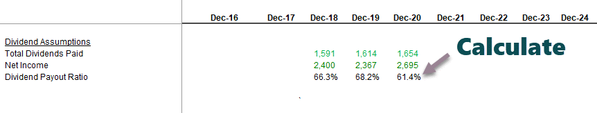
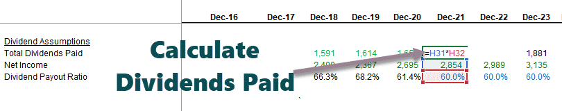
We note that the dividends payout ratio has been broadly in the range of 60%-66%. Therefore, let us assume the dividend payout ratio of 60% in the future years.
- We can also link the projected net income from the income statement.
- Using the projected net income and the dividends payout ratio, we can find the total dividends paid.
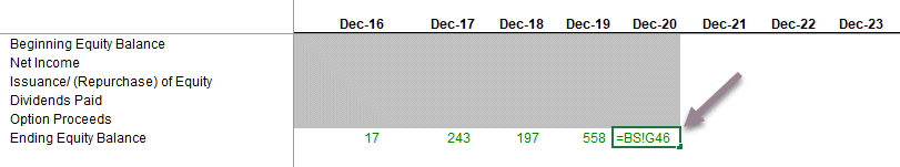
Forecast equity account in its entirety
With the forecast of share repurchase, option proceeds, and dividends, we are ready to complete the shareholder’s equity schedule. Link all these up to find the ending equity balance for each year, as shown below.
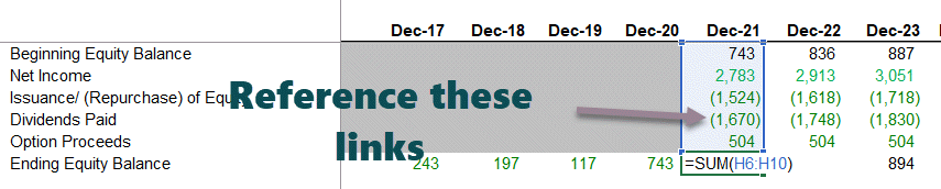
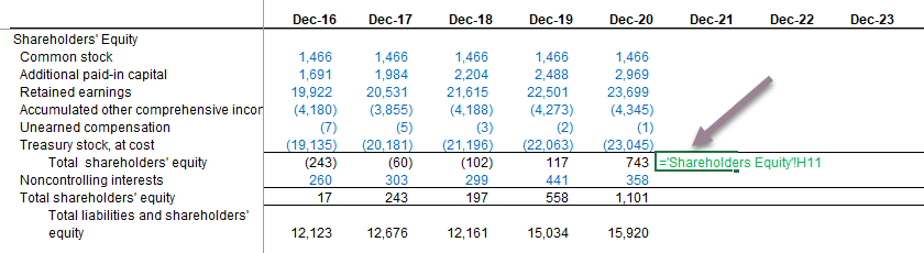
Link Ending Shareholder’s Equity to the Balance Sheet

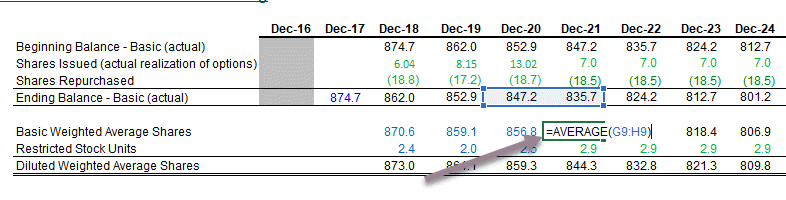
Step 10 – Shares Outstanding Schedule
The next step in this online financial modeling in Excel training is to look at the shares’ outstanding schedule. Summary of shares outstanding schedule:
- Basic Shares – actual and average
- Capture past effects of options and convertibles as appropriate
- Diluted SharesDiluted shares can be defined as the total number of shares that the company has at a particular point that can be converted into the normal share by the holders (convertible bond, convertible preferred stock, employee stock options). It is done by exercising the right to alter such shares into ordinary shares.read more – average
- Reference Shares repurchased and new shares from exercised options
- Calculate forecasted raw percentages (actual)
- Calculate average basic and diluted shares
- Reference projected shares to Income Statement (recall Income Statement Build up!)
- Input historical shares outstandingOutstanding shares are the stocks available with the company’s shareholders at a given point of time after excluding the shares that the entity had repurchased. It is shown as a part of the owner’s equity in the liability side of the company’s balance sheet.read more information
- Note: Commonly, this schedule integrates with the equity schedule.
Input the historical numbers from the 10K report
- Shares issuedShares Issued refers to the number of shares distributed by a company to its shareholders, who range from the general public and insiders to institutional investors. They are recorded as owner’s equity on the Company’s balance sheet.read more (actual realization of options) and shares repurchased can be referenced from the shareholder’s equity schedule.
- The input weighted an average number of sharesWeighted Average Shares Outstanding is a calculation used to estimate the variations in a Company’s outstanding shares during a given period. It is determined by multiplying the outstanding number of shares (consider issuance & buybacks) in a given reporting period with their individual time-weighted portions. read more and the effect of stock options for the historical years.
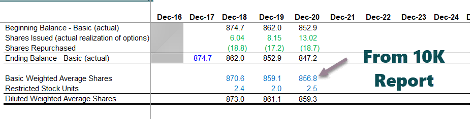
Basic Shares (Ending) = Basic Shares (Beginning) + Share Issuances – Shares Repurchased.
Find the basic weighted average shares
- We find an average of two years, as shown below.
- Also, add the effect of options and restricted stock units (referenced from the shareholder’s equity schedule) to find the diluted weighted average shares.
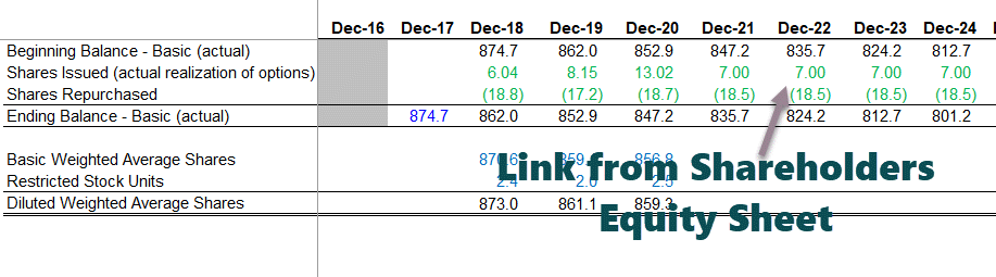
Link Basic & diluted weighted shares to Income Statement
- Now that we have calculated the diluted weighted average shares, it is time to update the same in the income statement.
- Link up forecasted diluted weighted average shares outstandingWeighted Average Shares Outstanding is a calculation used to estimate the variations in a Company’s outstanding shares during a given period. It is determined by multiplying the outstanding number of shares (consider issuance & buybacks) in a given reporting period with their individual time-weighted portions. read more to the income statement as shown below
With this, we complete the shares’ outstanding schedule and time to move to our next set of statements.
Step 11 – Completing the Cash Flow Statements
We must fully complete the cash flow statements before we move to our next and final schedule in this financial modeling, i.e., the debt schedule. Until this stage, there are only a couple of incomplete things.
- Income Statement – interest expense/ income are incomplete at this stage
- Balance Sheet – cash and debt items are incomplete at this stage
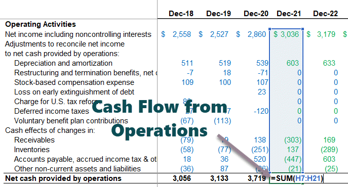
Calculate Cash Flow for Financing Activities

Also, check out Cash Flow from FinancingCash flow from financing activities refers to inflow and the outflow of cash from the financing activities like change in capital from securities like equity or preference shares, issuing debt, debentures or repayment of a debt, payment of dividend or interest on securities.read more
Find net increase (decrease) in Cash & Cash Equivalents

Complete the cash flow statements
Find the year-end cash and cash equivalents at the end of the year.
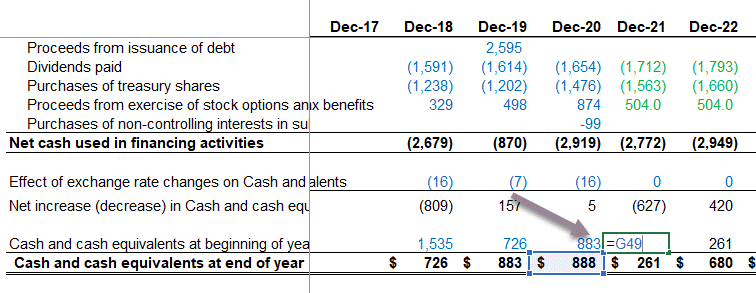
Link the cash & cash equivalents to the Balance Sheet.
Now we are ready to take care of our last and final schedule, i.e., Debt and Interest Schedule
Step 12 – Financial Modeling in Excel – Debt and Interest Schedule
The next step in this online financial modeling is to complete the debt and interest schedule. Summary of the Debt and Interest – Schedule.
Set up a Debt Schedule
- Reference the cash flow available for financing
- Reference all equity sources and uses of cash
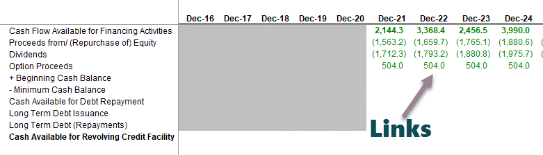
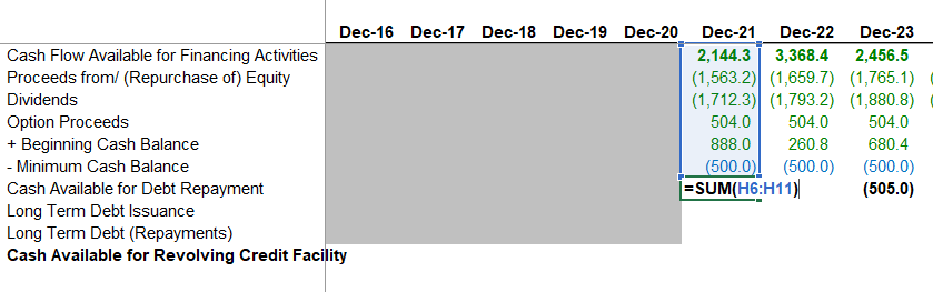
Calculate Cash Flow from Debt Repayment
- Reference the beginning cash balance from the balance sheet.
- Deduct a minimum cash balance. We have assumed that Colgate would like to keep a minimum of $500 million yearly.
Skip long-term debt issuance/ repayments, cash available for revolving credit facility, and revolver section.
Colgate’s 10K report notes the available details on the revolved credit facility.

Colgate 2020 – 10K, Page 49
Also provided in additional information on debt is the committed long-term debt repayments.
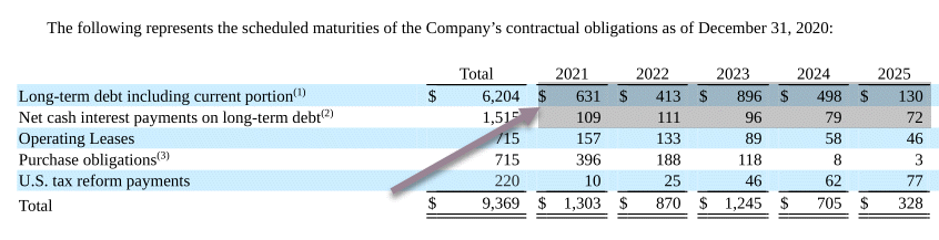
Colgate 2020 – 10K, Page 50
Calculate the Ending Long Term Debt.
We use the long-term debt repayment schedule provided above and calculate the ending balance of long-term debt repayments.
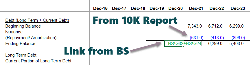
Link the long term debt repayments
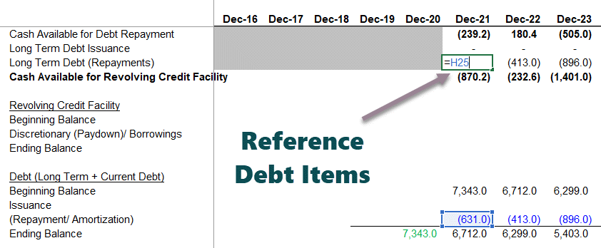
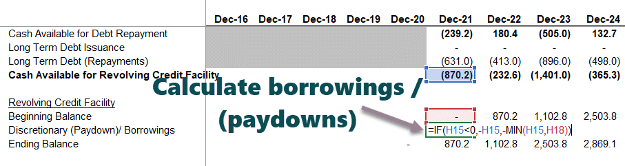
Calculate the discretionary borrowings/paydowns.
Using the cash sweep formula, as shown below, calculate the discretionary borrowings/paydown.
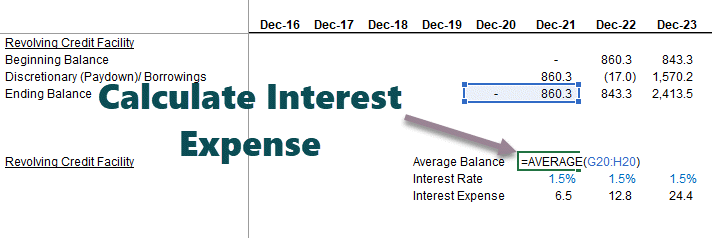
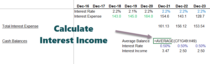
Calculate Interest Expense from Revolving Credit Facility
- Make a reasonable assumption for an interest rate based on the information provided in the 10K report.
- Find the average balance of the revolving credit facility and multiply it with the assumed interest rate.
Calculate the Interest Expense from the Long Term Debt
Link the historical average balances and interest expenses. Find the implied interest rate for historical years.
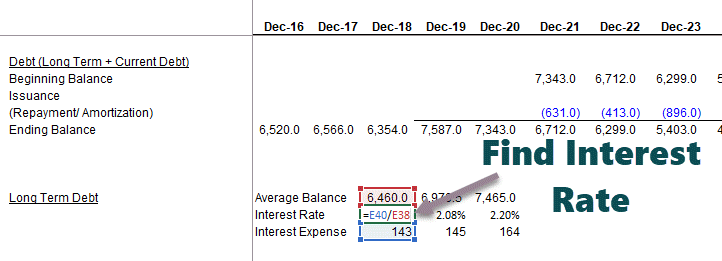
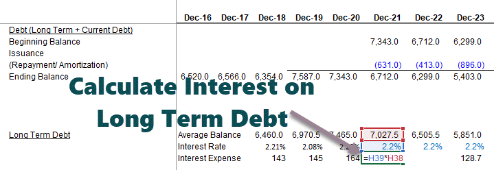
Assume the interest rate on Long term debt based on the implied interest rate. Then, multiply the average long-term debt by the assumed interest rate.
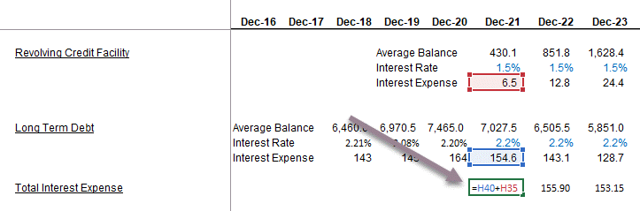
Calculate Total Interest Expense = average balance of debt x interest rate
Find the Total Interest Expense = Interest (Revolving Credit Facility) + Interest (Long Term Debt)
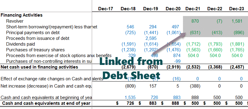
Link debt & Revolver drawdowns to Cash Flows
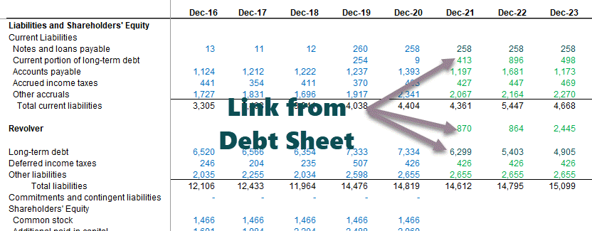
Reference Current and Long Term to Balance Sheet
- Demarcate the Current Portion of Long Term DebtCurrent Portion of Long-Term Debt (CPLTD) is payable within the next year from the date of the balance sheet, and are separated from the long-term debt as they are to be paid within next year using the company’s cash flows or by utilizing its current assets.read more and long-term debt as shown below.
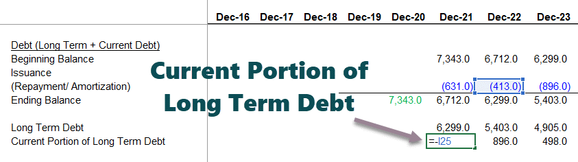
- Link the revolving credit facility, long-term debt, and current portion of long-term debt to the balance sheet.
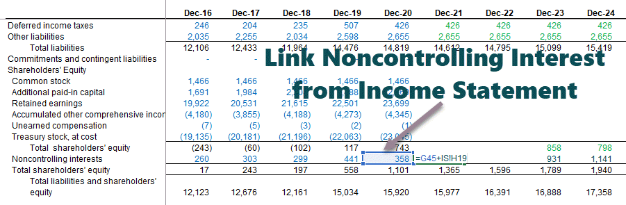
Link Noncontrolling Interest from Income Statement
Calculate the Interest Income using the average cash balance
Link Interest Expense and Interest Income to Income Statement

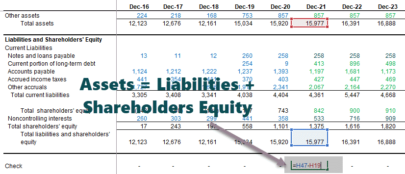
Perform the Balance Sheet check: Total Assets = Liabilities + Shareholder’s Equity
Audit the Balance Sheet
We need to audit the model and check for linkage errors if there is any discrepancy.
Recommended Articles
- Alibaba Financial Model
- Box IPO Financial Model
- Financial Modeling Templates
- Coursera Financial Model
What next?
If you learned something new or enjoyed this Excel-based financial modeling, please leave a comment below. Let me know what you think. Many thanks, and take care. Happy Learning!
The production cost calculation of production is the determination of costs in terms of money per unit of goods, works or services. The calculation includes direct and indirect costs. Direct is the cost of materials, wages of workers, etc. Indirect costs: planned profit, transportation, etc.
We will not consider calculating articles in detail. We automate the process of calculating the planned production cost of production using Excel formulas. Our task is to create a table using Excel tools so that when you substitute data, the production cost of goods, works, and services is automatically considered.
The production cost calculation of goods in trade
It is better to learn how to calculate the production cost price from the sphere of trade. There are fewer costs. In fact — the purchase price, issued by the supplier; transportation expenses for the delivery of goods to the warehouse; duty and customs fees, if we import goods from abroad.
We take a certain group of goods. We calculate the production cost price for each of them. The last column — the planned production cost factor — will show the level of costs that the company will incur for the delivery of products.
We fill in the table:
- Transportation costs, according to the logistics department, will be 5% of the purchase price.
- The amount of the duty will vary by different groups of goods: for the goods 1 and 4 — 5% and for the goods 2 and 3 — 10%. To make it more convenient to set percentages, we sort the data by the column «Name of product».
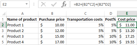
- For the calculation we use the formula: the purchase price + transport costs in monetary terms + duty in monetary terms.
- The formula for calculating the planned ratio is the production cost price in monetary terms / purchase price.
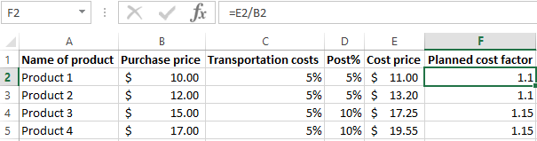
The level of costs for the delivery of goods 1 and 4 will be 10%, 2 and 3 — 15%.
Formulas for calculation the planed production cost of the production in Excel
Each company calculates the planned production cost in its own way. After all, enterprises bear different costs depending on the type of activity. Any calculation must contain a decoding of the costs of materials and wages.
The calculation of the planned production cost price begins with the determination of the production cost of raw materials and materials used for the production of goods (which are directly involved in the technological process). The expenses of raw materials is included in the expenses of the standards approved by the enterprise minus technological losses. These data can be taken in the technological or production department.
We will reflect the norms of raw material consumption in the Excel table:
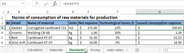
Here we managed to automate only one column which is the column with the expense taking into account the technological losses. The formula is = E3 + E3 * F3.
Note! For the «Technological losses,%» column, we set the percentage format. Only in this case the program will calculate correctly. The numbering of the lines begins above the header. If the data is messed up, you can restore them by numbers.
Knowing the norms, we can calculate the cost of materials (the calculation is for thousands of items):
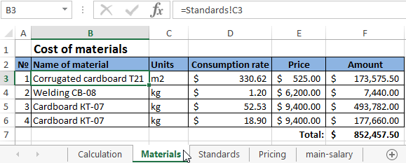
In this table, you have to manually fill in only one column – «Price». All other columns refer to the data of the «Standards» sheet. In the column «Amount» the formula works: = D3 * E3.
The next article of direct costs is the wages of production workers. The basic salary and additional are taken into account. The principles of the salary is charged (piece-work, time-based, from output), you can find out in the accounting department.
In our example, the calculation of wages is carried out according to the norms of output: how much an employee of a certain qualification must make for a unit of working time.
Data for calculations are as follows:
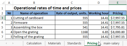
The price is calculated by the formula: = C3 * D3.
Now we can calculate the basic salary of workers:
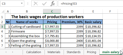
To fill the first two columns, not including the number in order, we linked the data of this table to the data of the previous one. The formula for calculating the bonus is = C3 * 30%. The basic salary is = C3 + D3.
Additional wages are all payments made by law, but not related to the production process (holidays, remuneration for long service, etc.).
Other data for calculating the production cost of production we added to the table immediately:
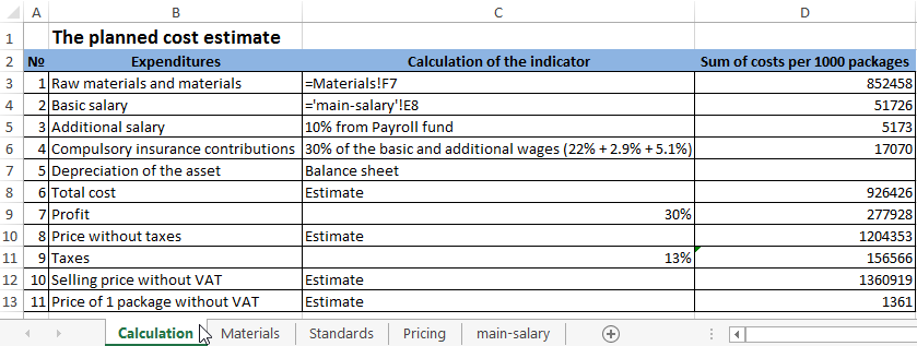
The column «Calculation of the indicator» indicates the place we are taking the data from. If we refer to other tables, then we use the resulting sums.
To estimate the calculation of the production cost of packages, conditional indicators of OS depreciation, percentages of additional wages and taxes, mandatory insurance premiums are taken.
The formula for calculating the expenses of a product with formulas:
- Download cost calculation in Excel
- Calculation of production costs with data
- Calculation of production costs with norms
- Example of costing with overhead
Любой бизнес-план нуждается в финансовых расчетах. А наиболее удобный инструмент для этого – табличный процессор Excel. Популярность программы объясняется простотой использования и многофункциональностью. Рассмотрим возможности редактора, которые будут полезны при составлении бизнес-модели.
Основы построение финансовой модели в Excel
Модель можно поместить на один лист или на разные листы. В любом случае, порядок расчетных таблиц должен соответствовать логике описания проекта:
- таблицы для расчета инвестиций;
- доходная и затратная часть;
- финансирование;
- итоговые отчетные формы, показатели.
Инвестиционный план
Основные элементы:
- строительство и/или покупка зданий;
- покупка оборудования;
- расходы будущих периодов;
- инвестиции в ЧОК (чистый оборотный капитал).
Исходные данные для расчета затрат на покупку или строительство зданий:
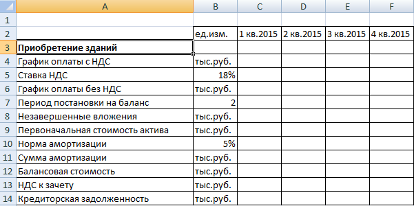
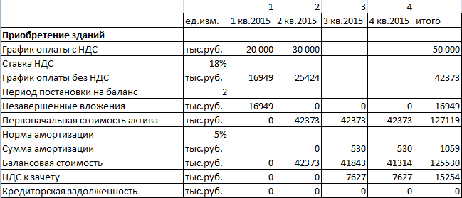
Расчеты:
- График оплаты без НДС = Затраты с НДС / (1 + ставка НДС). Формула в Excel для ячейки С6: =C4/(1+$B$5).
- Незавершенные вложения – сумма вложений в активы без учета НДС до периода их постановки на баланс. Формула в Excel для ячейки С8: =ЕСЛИ(C1<$B$7;СУММ($C6:C6);0).
- Сумма амортизации начисляется со следующего периода. Формула в Excel для ячейки D11: =ЕСЛИ(D1>$B$7;ЕСЛИ(C12>0;ЕСЛИ(D9*$B$10/4>C12;C12;D9*$B$10/4);0);0).
- Балансовая стоимость актива – разница между начальной стоимостью и амортизационными отчислениями за весь период существования актива. Формула в Excel для ячейки D12: =D9-СУММ($C11:D11).
- Формула для расчета первоначальной стоимости актива — =ЕСЛИ(C1>=$B$7;$G$6;0).
- НДС к зачету (в период постановки актива на баланс) – общая величина налога. Формула для ячейки С13: =ЕСЛИ(C1>$B$7;$G4-$G6;0).
- Формула для расчета кредиторской задолженности: =ЕСЛИ(C1>=$B$7;$G6-СУММ($C6:C6);0).
Затраты на приобретение оборудования и элементы расходов будущих периодов в инвестиционном плане составляются аналогично. Особенности затрат будущих периодов:
- оприходуются на баланс в составе текущих активов;
- не облагаются налогом на имущество (в отличие от оборудования);
- амортизируются быстрее, в течение 1-2 лет.
Прогнозирование доходов
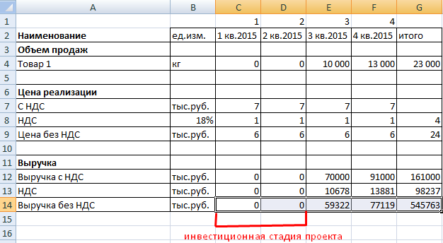
Чтобы построить план продаж, нужно определить объем в натуральном выражении (для каждого вида продукции) и цену реализации (каждого вида продукции). Выручка определяется по каждому виду товара (работ и услуг) как произведение объема и цены.
В Excel составляются таблицы для каждого периода планирования и для каждого вида продукции с планируемым объемом выпуска (в натуральных единицах).
Из цены реализации нужно вычленять сумму налога на добавленную стоимость. Эти деньги не входят в состав выручки – они перечисляются в бюджет.
Формулы:
- Цена без НДС = цена с НДС / (1 + налоговая ставка).
- Величина НДС = (цена с НДС * налоговая ставка) / (1 + налоговая ставка).
Расчетная таблица может выглядеть следующим образом:
- Формула для расчета цен без НДС: =C7/(1+$B$8).
- Расчет налога на добавленную стоимость: =C7-C9.
- Выручка с налогами: =C4*C7.
План текущих расходов
Элементы затрат:
- сырье и материалы;
- оплата труда;
- начисления на зарплату;
- амортизация;
- прочие расходы.
При учете затрат на материалы выделяем налог добавленной стоимости. Это необходимо для учета подлежащих возврату сумм (задолженность перед бюджетом уменьшится).
Затраты на сырье и материалы увеличиваются прямо пропорционально объему выпуска. Если, к примеру, на пошив одной сорочки требуется полтора метра ткани, то на две единицы продукции – 3 метра и т.д. Расход считается по формуле:
Количество материалов = удельный вес * объем производства.
Пример таблицы учета текущих затрат на сырье и материалы:
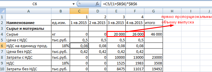
Формула для расчета налога на добавленную стоимость – в строке формул.
Формула вычисления цены без НДС: =C5/(1+$B$6).
Расчет затрат с НДС: =C4*C5.
Налог на ДС: =C4*C6.
Затраты без НДС: =C4*C7.
Прочие расходы:
- аренда,
- реклама,
- оплата связи;
- ремонт и т.д.
При составлении финансовой модели предприятия в Excel учитывается каждая статья расходов.
Финансовая модель предприятия в Excel
Когда спланированы продажи и затраты, можно приступать к формированию баланса, плана доходов и расходов, движения денежных средств. Чтобы модель пересчитывала значения в автоматическом режиме, данные в сводных отчетах рассчитываются с помощью формул или напрямую извлекаются из операционных планов (с помощью ссылок).
План доходов и расходов финансовой модели:
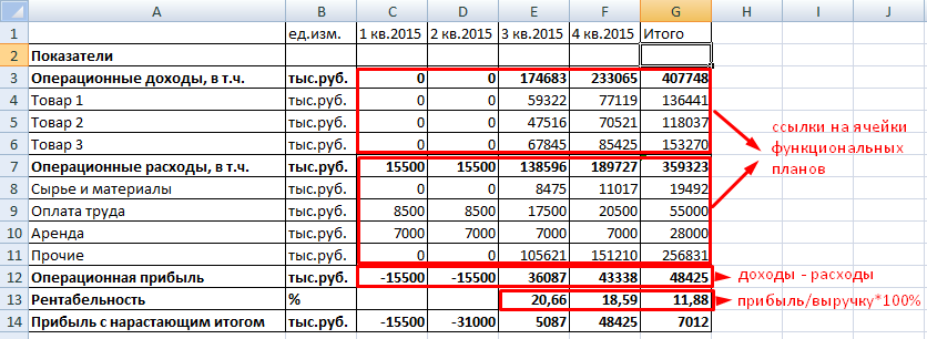
Доходы и расходы расписаны по статьям. Если планируется выпуск десятков наименований продукции, то лучше определить их в группы. Чтобы не перегружать отчет. В сводную таблицу добавлены аналитические показатели: рентабельность и прибыль с нарастающим итогом. Когда нужно больше аналитики, формируют отдельные таблицы.
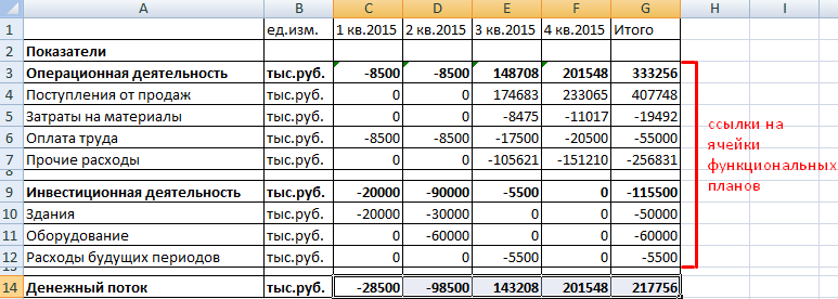
План движения денежных средств:
Скачать пример финансовой модели предприятия в Excel
По теме: Финансовая модель в Excel при покупке бизнеса.
Предполагается, что предприятие не будет привлекать заемные средства. Поэтому раздел «Финансовая деятельность» отсутствует.
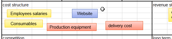
Business Models 101: Cost Structure
In this part we will discuss the Cost Structure, which includes
everything (people, services, material, tax,…) that drains money out of
your company.
I have to repeat it on every page but starting something on your own, creating value for you, your family and
the world is a totally recommendable thing to do. You want to create your
company. This is GREAT. The world has been made by
people like you. Entrepreneurs. Self-Made Men, Creators, Builders people
that believed an obstacle is just another great challenge to overcome, to
solve and put behind them as an achievement.
The Cost Structure
Costs are the part you do not like to have in a company.
Having no cost is always better. But this is impossible. Producing
something will always cost, even the electricity to light your room, the
internet service provider to promote your products, etc…
Under cost
structure you have to list all the items that are draining your company from
its cash. These costs have to be minimized at all «cost».
But do not do the mistake of trying to save where it is not necessary
or opposite: save where it is necessary.
For example, let’s say your cupcake factory
start making money and you need to fill you the tax return. If this takes
you too much time, then hire an accountant to make it for you. You should
use the rule of thumb that is: every work that takes me away from creating
value and that takes more than 5% of my time, should be subcontracted.
Example: you work 60 hrs. in a week, which is a lot, then
you should not spend more than 3 hours on stuff that is not essential,
because there are other essential things in your life currently. And resting
a bit is also very important.
Trying to do
something yourself instead of using someone else or subcontracting lets you focus
on the important actions you have to do for your company.
Here are the questions you have to ask yourself
about the Cost Structure:
Which resources are costing the most? Can you save here or
not?
Which activity is costing the company money? Is this an
essential activity or not?
How is our
cost structure built? What are the repartition (fixed, variable,
franchise cost, etc…)?
What is costing you the most, how useful is it to your business?
Are the revenues higher than the
costs? Hopefully so, but may be at the beginning you still are in the red
because you need more sales to make break even.
Can investments be paid back? Look at this carefully because
banks and investors are usually not lenient and nice and also have no
patience.
Typical costs are:
- Equipment,
- wages
- salaries
- taxes
- consumables (ingredients, packaging, ….)
- transportion
- building
-
uniform,
gear - cleaning equipment
- vehicles
Previous: Key Partners
Next: the long term goal,
mission, strategy
Download the
excel business model canvas Template from here.
Please Tweet, Like or Share us if you enjoyed.
Imagine you are the in-charge of finance department at Hogwarts. So one fine day, while you are practicing the spells, Dumbledore walks in to your office and says, “Our electricity bills are way too high. As the muggles don’t accept wizard money, we have to find a way to reduce our power consumption.”
So you summoned the previous 12 month utility bills to examine energy consumption patterns, and pretty soon you realized that most of the electricity consumption is due to the light bulbs. You suddenly have a brilliant idea. Why not replace the light bulbs with a variety that consumes low power? A light bulb moment indeed.
Your next step is to figure out what varieties of light bulbs are out there. Fortunately this is easier than catching a snitch in a game of quidditch. A quick search revealed that there are 3 types of light bulbs:
- Regular incandescent bulbs (the kind Hogwarts currently uses)
- Compact Fluorescent Light bulbs (CFL)
- Light Emitting Diode bulbs (LED)
Now your job is to do a cost benefit analysis of these options and pick one.

What is cost benefit analysis & how to do it?
Cost benefit analysis, as the name suggests is a process of identifying all the costs & benefits of different decision choices and finding which choice offers maximum benefit for minimum cost.
It is a generic technique and the implementation varies depending on situation, industry and available data.
A typical cost benefit analysis involves these steps:
- Gather all the necessary data
- Calculate costs
- Fixed or one time costs
- Variable costs
- Calculate the benefits
- Compare costs & benefits over a period of time
- Decide which option is best for chosen time period
- Optional: Provide what-if analysis
Let’s conduct cost benefit analysis for our light bulb problem and figure out which option is best.
But first, download the cost benefit analysis workbook
Click here to download the cost benefit analysis workbook. Refer to it as you read this article for best results.
1. Input Data & Assumptions
For each type of bulb we need to find out below information:
Costs:
- Price
- Electricity consumption (watts/hr)
- Life time in hours
Benefits:
- Amount of light (lumens) generated by the bulb
Assumptions:
We also need to assume a few things to keep our cost benefit analysis model realistic & simple.
Some of the assumptions we can go with are,
Global assumptions:
- We need only 1 bulb (doing analysis for n bulbs is just a matter of multiplying 1 bulb results with n)
- Analysis will be conducted in Indian Rupees
- Let’s compare bulbs that give same amount of light (lumens). This means we can ignore the benefit part and focus on costs alone
- This analysis ignores any impact / costs / benefits associated with environmental impact (CO2 emissions, harmful metals like mercury, heat generation etc.)
- Analysis time frame is 5 years.
Other assumptions:
- Average usage of bulb per day is 8 hours.
- Cost of electricity is Rs. 5 per unit (KWH)
- Inflation for electricity cost is 1%
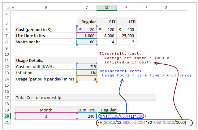
Once we have all the data, tabulate it in Excel like this:

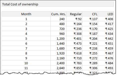
2. Calculate Total Cost of Ownership
Once we have all the necessary data, let’s calculate the total cost of each option (Regular, CFL & LED) over a period of 5 years.
This step involves calculating both fixed & variable costs.
Fixed or one time costs:
The fixed cost for each light bulb type is nothing but the price.
But wait… what about the life time of bulb?
Since each type of bulb has certain life time, we will have to pay for replacement of bulbs too.
This means, apart from fixed cost at the start of time period, we will also have a variable cost that depends on the life time of bulb type.
Variable costs:
There are 2 variable costs in our analysis.
- Electricity consumption cost
- Bulb replacement cost
Electricity consumption cost:
This is calculated by below formula:
Wattage per month / 1000 * Inflated unit cost
The actual Excel formula looks like this:
FV($C$13/12,$B20,-$C$14*30*C$8*$C$12/1000)
How this formula works?
To understand this formula, first imagine what the total unit cost should be at the end of Month x.
For first month, the cost is =total monthly usage in hours * watts per hour / 1000 * unit cost * (1 + inflation/12)^1
For second month, the cost is same as above, but the exponent in the end becomes 2.
Let’s say, the blue part of the formula is denoted by something.
Then, the cost at the end of Month X will be,
=something * ( (1+inflation/12)^1 + (1+inflation/12)^2 + … + (1+inflation/12)^X )
Oh, all this math is confusing… Isn’t there a simple spell to answer this?
I am glad you asked. There is a spell to get this answer in one shot. It is called as FV()
The FV formula calculates sum of above series.
We simply write
= -FV(inflation/12, month number, total monthly usage in hours * watts per hour / 1000 * unit cost)
to get the answer we want.
Why the minus sign in front of FV?
This is because, by default FV returns values in negative. It has got something to do with how banks always take money from us, but are very reluctant to give back or like that.
Bulb replacement cost:
The unit cost formula felt like trying to catch a snitch while riding a broomstick upside down. Thankfully, the bulb replacement cost formula feels like sitting in the crowd, cheering match while eating chocolate frogs.
The calculation for bulb replacement goes like this:
Cumulative usage in hours / life time of the bulb * unit price of bulb
Here is the formula for this:
(INT(cumulative usage/ life time of the bulb)+1)*unit price of bulb
Why use INT(…) + 1
Let’s say the life time is 1,000 hrs, cost is Rs 20 and we use 240 hrs in first month. Our cost is still Rs. 20, not 24% of 20.
Likewise, at the end of 5th month, our total usage would be 1200 hrs (240 x 5 = 1200) and we must buy a new bulb as the life time is only 1000 hrs.
The replacement cost is not uniformly spread across months (or hours). It happens once at beginning and then recurs once per lifetime of the bulb.
Hence we use INT to round the cumulative usage / life time to the integer portion (ex: INT(240/1000) will be 0) and add 1 to it as there is initial cost.
Explanation of these formulas in our spreadsheet
Look at below illustration to understand how these formulas look in the cost benefit analysis worksheet.
3. Calculate benefits
This part is not required for our problem as the benefits are same for all 3 types of bulbs. You can use logic similar to cost calculation when the benefits vary. For example if you want to do cost benefit analysis of 3 types of investment choices – mutual funds, stocks, bank deposits, then you can use below framework:
Costs:
- Brokerage costs
- Entry costs
- Operating expenses
- Exit costs
- Volatility / risk factors
Benefits:
- Return of the investment
- Liquidity benefit
4. Compare costs & benefits over a period of time
Once we have these cost & benefit calculations ready, we need to calculate them for 60 months (5 years) for all 3 types of bulbs.
The resultant table looks something like this:
5. Decide the winner
Once we have all the numbers, it is just a matter of picking the winner. If you are comparing costs, pick the lowest cost item. If you are comparing benefits, pick the item that offers most benefit / cost ratio.
How to convince your boss about the decision?
While it is easy to decide which option is the winner by just looking at numbers, when you take this proposal back to Dumbledore, he may want a little more explanation. This is where a visualization of cost benefit analysis can help.
Example – Visualization of Cost benefit analysis
Here is a completed visualization of our light bulb cost benefit analysis.
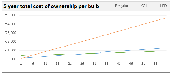
How to create this chart?
Simple, just follow below steps.
- Select the total cost of ownership table that you calculated
- Insert a new line chart
- Format the chart as per your (or your boss’) taste
- Done
Things to keep in mind:
- Go with line charts if your analysis is against a time period or similar
- Go with column / bar charts if you are comparing various options with one time costs only
- Format the chart so that it is easy to identify winning choice at each point of time.
Adding what-if analysis
What if analysis is a great way give power to your decision makers. When you prepare a cost benefit analysis model like above, you will always hear questions like:
- So what would be the total cost for using 12 CFL bulbs 16 hours per day for next 25 years?
- In above case, how much would we save if we switch to LED bulbs?
- What would be the cost for 30 years? 10 hours a day? 20 bulbs?
Thanks to powerful Excel form control feature, you can easily add a comprehensive what-if analysis tool to your model.
Like this:
Process for adding what-if analysis
Follow below process for including what-if analysis in your spreadsheet models.
- Identify all possible scenarios for which what-if analysis may be required.
- Determine the variables (in our case, the variables are number of bulbs, bulb type, usage in hours & years)
- Figure out what output should be displayed (in our case, the output is total cost and a comparison with other bulb types)
- Set up an input area where user can select any combination of variables
- Use form controls, slicers, data validation, VBA or simple input cells for gathering this data
Tip: click on those linked words to understand how to set them up - Write formulas that link to the user input cells / form controls
- Display the output (text, charts etc.)
Please examine the download workbook for actual implementation of this.
Guidelines for creating better analysis models
Whenever you are analyzing something like this, please follow below guiding principles for awesome results.
- Do your research first: Identify all factors, inputs, assumptions & facts that impact the decisions. Spend sometime researching before jumping in to Excel.
- Set up separate areas of input, analysis & output: Create separate areas in your workbook to handle inputs, calculations & outputs (such as charts, text). Clearly demarcate them by using different styles or headers for each section.
- Avoid analysis paralysis: Keep your analysis workbooks simple & realistic. Don’t over complicate them with too many inputs or too much calculation. If a certain factor is irrelevant or too complicated to consider for your analysis, ignore it. Example: in our analysis we ignored benefits as they are same for all 3 options. We also ignore environmental impact as it is tricky to calculate.
- Use consistent formulas: Write your formulas in such a way that same pattern is repeated many times. This way you can write once and use the power of relative & absolute references in Excel to fill the formulas everywhere.
- Let users play with your model: Include what-if analysis or form control based interaction in your workbooks so that your users can play with the model and get answers for their questions.
- Visual explanations: Visual explanations like charts, dashboards are very powerful & memorable. So depict your results visually as much as possible. Remember the old adage, a picture is worth thousand words.
Related: Spreadsheet modeling best practices for analysts
Download Cost Benefit Analysis workbook
Please click here to download cost benefit analysis workbook. Examine the calculations & form controls to learn more.
Cost benefit analysis – your experiences please…
Cost benefit analysis was a big part of my work when I worked as an analyst. Now I am in the role of a CEO and it is even more relevant for me. For most situations I create a simple Excel model to examine the costs & benefits to decide the winner.
What about you? How do you analyze costs vs benefits? What techniques do you use? Please share your stories, examples & tips in the comments section.
Want more? Introducing 50 ways to analyze data course
If you like to learn how to analyze data, gather insights, prepare outputs & interpret results, then you will love my new course – 50 ways to analyze data.
The above example is lesson number 24 in our course. Each of the 50 lessons deal with common business analysis situations, case studies & techniques so that you can become the analytical wizard you always wanted to.
This course is now open.
If you want to know more about it, please click here.
Инструмент финансового моделирования бизнес-проекта создан как
обычный Excel файл без макросов и скриптов. Его можно
копировать, переносить,
передавать, использовать для работы
несколькими сотрудниками, но при этом необходимо
соблюдать правила коллективной работы при использовании Excel.
Файл выполнен в виде законченного продукта, не требующего
доработки. Это шаблон финансового моделирования, который при
внесении в него исходных данных автоматически рассчитывает
необходимые финансовые показатели и генерирует необходимые для
бизнес-планирования отчеты.
Шаблон можно использовать многократно для различных профильных
проектов.
Для создания финансовой модели необходимо в Excel шаблон внести:
-
Общие исходные данные проекта;
-
Данные о продажах.
Рекомендуем перед началом заполнения шаблона финансовой модели
собрать исходные данные в
отдельном файле.
Для удобства просмотра разверните видео на полный экран.
Данные о продажах для финансовой модели
Создайте краткое описание вашего товара или услуги, заполнив
следующие данные для финансовой модели:
-
Наименование продукта или услуги;
-
Цена по которой продажи продукта или услуги;;
-
План продаж;
-
Количество продаваемого товара и дата начала продаж.
Для удобства просмотра разверните видео на полный экран.
Механизм управления планом продаж позволяет:
-
Быстро спланировать ежемесячные продажи, рассчитать
равномерное изменение цены и количества реализуемого товара
или услуг во времени с учётом сезонности и ограничений периода
продаж; -
Построить нелинейный план продаж в денежном выражении. Изменяя
ежемесячный показатель в процентах, вы формируете свое видение
на реализацию товаров и услуг; -
(НОВОЕ) Свободное планирование планом продаж
в количественном и денежном выражении исходя из начальной
стоимости продукта или услуги;;
Для использования инструмента свободного планирования:
-
Перейдите в раздел «Продукты», установите
название реализуемого продукта, цену за единицу товара или
услуги, количество реализуемых в месяц и дату начала продаж; -
Выберете столбец «План продаж». Функция
подключает дополнительный инструмент расчета в данном разделе. -
Перейдите в подраздел «План продаж». Вы
увидите две колонки таблиц:
левая —
управляем продажами путем установки объема продаж в
процентах,
правая — управление
продажами путем произвольного определения количества
реализуемого товара или услуг в месяц.
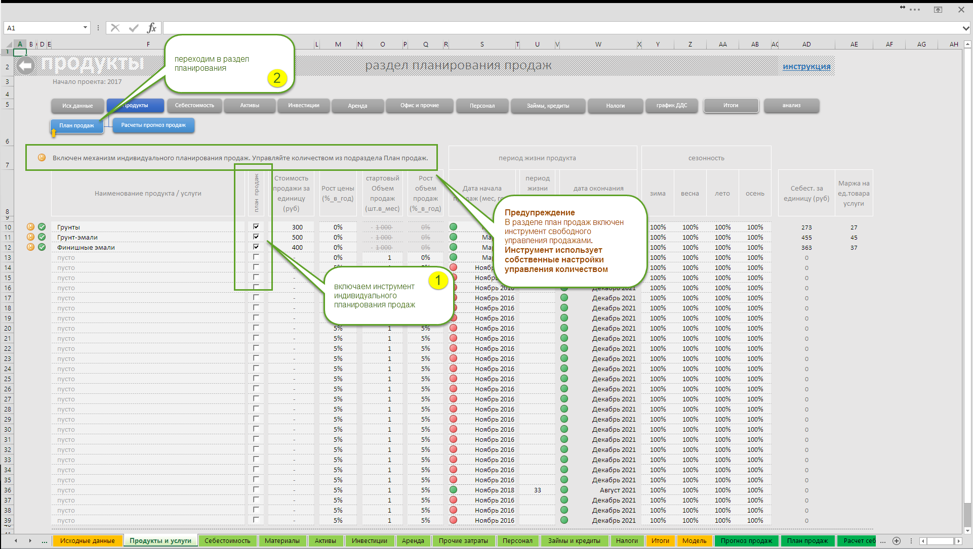
ВАЖНО! Для использования
нужного способа планирования необходимо произвести переключение
между таблицами инструментом select.
Данные о затратах для финансовой модели
Затраты разделены на несколько групп, каждая из которых
предполагает наличие минимального необходимого объема информации,
позволяющий учесть 99% затрат вашего проекта. Руководствуйтесь
разумной достаточностью чтобы создание финансовой модели в Excel
не стало обременительным.
Группы затрат финансовой модели
Для создания финансовой модели в Excel необходимо ввести в шаблон:
-
1. Себестоимость
Самый очевидный вариант использования раздела – производство.
Определяем затраты, связанные с созданием единицы продукта или
услуги. Если выделить затраты за единицу товара невозможно, то
планируем закупки материалов с заданной периодичностью. Для
проектов, связанных с продажей услуг, или проектный бизнес не
всегда можно выделить себестоимость затрат. В этих случаях
раздел может не заполнятся.Для удобства просмотра разверните видео на полный
экран. -
2. Активы
Недвижимость, оборудование, автотранспорт, средства
производства без которых ваш продукт или услугу произвести
невозможно. Планируем затраты, обеспечивающие бизнес
средствами производства и(или) оказания услуг. Покупаем
здание, станки, дорогостоящую оргтехнику, лицензии, проектную
документацию. Всё, что составляет материальную ценность
проекта размещаем в данном разделе.
(см. видео ниже) -
3. Инвестиции
Купленный актив нужно обслуживать, ремонтировать, планировать
его модернизацию. Эти данные заполняем в данном разделе.
Информация для планирования затрат в раздел
«инвестиции» попадают автоматически из
раздела активы, планирование не займет много времени. Подробно
об этой группе рассказано в видео инструкции по созданную
финансовой модели.
(см. видео ниже) -
4. Аренда
Аренда офиса или оборудования. В финансовом плане аренда
позволяет экономить существенные денежные средства. Старайтесь
оптимизировать затраты чтобы стимулировать продажи, и не
тратить деньги там, где можно этого не делать в данный период
времени.
(см. видео ниже) -
5. Офис
Затраты на обеспечение бизнеса – важная часть финансового
планирования. Коммунальные платежи, ИТ поддержка, транспортные
и рекламные расходы, вода в офис, кофе и чай. Эти и многие
другие затраты обеспечивают ежедневные будни бизнеса. Обратите
внимание: сюда не стоит включать затраты, являющиеся вашим
коммерческим продуктом.
Например «реклама». Если ваш бизнес — реклама, то реклама –
ваш продукт. Затраты на рекламу переходят в
«Себестоимость».Для удобства просмотра разверните видео на полный
экран. -
6. Персонал
Должности, затраты на оплату труда сотрудников, распределение
затрат во времени, схемы и фонд оплаты труда.
(см. видео ниже)Инструмент планирования ФОТ имеет простой и удобный интерфейс
заполнения исходных данных. Обязательные поля для заполнения:-
Строка для указания должности. Если данная строка не будет
выбрана, то расчет указанных цифровых значений исключится
из расчёта. -
Укажите размер оклада на старте проекта, размер индексации
и дату начисления. -
Если работник имеет срочный контракт, используйте поле
«Период найма» для указания длительности
в месяцах. -
Если предполагается вознаграждение, в зависимости от
результатов работы проекта, воспользуйтесь колонкой
«Cхема начисления оклада» и установите
один из вариантов:-
только оклад;
-
оклад + процент от оборота;
-
только процент;.
-

-
-
7. Налоги
Налоги часть затрат, без них расчёты финансовой модели будут
неполными. Раздел «Налоги» позволяет оценить
необходимые суммы для удовлетворения налоговых органов. Размер
базовых ставок в РФ уже предустановлен. Вы самостоятельно
можете выбрать налоговый режим, размер ставок, применительно к
тому региону в котором проект будет реализован.Для удобства просмотра разверните видео на полный
экран. -
8. Займы и кредиты
Если задумались о поиске инвестора, значит планируемый к
реализации проект испытывает дефицит денежных средств. После
того, как закончили вводить план продаж и затраты шаблон
финансовой модели автоматически рассчитает потребность проекта
во внешнем финансировании. Данный раздел позволяет понять
сколько не хватает, оценить период и эффективность будущих
вложений, запланировать кредитование (внешнее финансирование).Для удобства просмотра разверните видео на полный
экран. -
9. Итоги и отчетность
Результатом планирования становятся автоматически
сформированные отчеты:-
Прибыли и убытки;
-
Движение денежных средств;
-
Прогнозный баланс;
-
Расчет инвестиционных показателей;
-
Расчёт точки безубыточности.
Для удобства просмотра разверните видео на полный
экран. -
-
10. Создание прогнозов
Обязательным для бизнес-планирования является создание
прогнозов: реалистичного, оптимистичного, пессимистичного.
Закончив процесс моделирования, вы создали «реалистичный»
прогноз. Сохраните файл два раза под другими именами,
например:
оптимистичный.xlsx, пессимистичный .xlsx, и
приступайте к созданию прогнозов. (см.видео)Для удобства просмотра разверните видео на полный
экран.
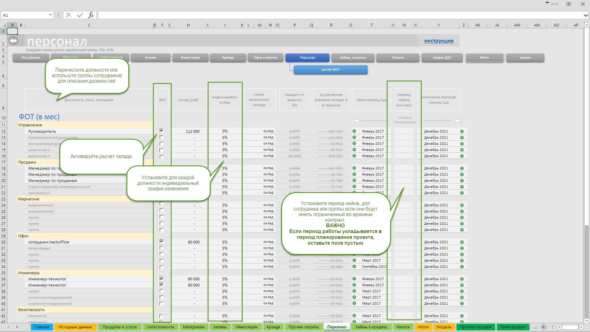
Полная видеоинструкция по созданию финансовой модели в Excel
Весь видеоматериал в одном файле. Для получения целостного
представления об использовании шаблона финансовой модели в Excel
смотрите полный видеоматериал.
Для удобства просмотра разверните видео на полный экран.
This tutorial will show you how to create a Project Finance Model and forecast Cash Flow in Excel with step-by-step instructions, practical examples to download and the calculation of Equity Investment Returns.
First, I will take you through building a simple cash flow forecast for a generic project. Then, I will use that spreadsheet to create a consolidated cash flow financial model. Lastly, I will show how to use those cash flows to calculate return on investment and then see how changes in assumptions impact your overall equity returns.
Download my Project Finance Model Template in Excel to follow the examples from this tutorial.
Step 1. Start with a Cash Flow Template for One Project
To create a Project Finance Model in Excel, start with an empty spreadsheet and type in month numbers in one of the first rows. I will be building a monthly cash flow model spread over ten years, so my model will have 120 columns, with one for each month.
Then, below the month rows, add the main drivers of the model, for example, the number of units added or built. For simplicity, I will assume that each unit represents a connected home (for example, a house connected to a fibre or broadband internet network). You could also easily define the driver as a unit of length (for example, the length of the electricity grid) or any other meaningful metric.
Lastly, to make your project finance model user-friendly, use Excel’s freeze panes functions to see what period you are looking at as you scroll through the spreadsheet.
Step 1. An Example of a Cash Flow Template and Revenue Forecast for Project Finance. Download the full Excel file here.
Step 2. Forecast Direct Cost and Revenues in Project Finance
To calculate Direct Revenues in a Project Finance Model, you will need to connect the drivers with the model’s Revenue and Cost assumptions.
For example, if the model assumes 100 new units connected in month one and the upfront fee is $100, the total upfront revenue in that month would equal $10,000 (i.e. 100 new units x $100).
Similarly, link a unit cost assumption to the drivers to calculate Direct Costs. For example, to calculate marketing cost, my Project Finance Model Template takes the number of new units and multiplies it by the cost per acquisition assumption.
Step 2. An example of Direct Cost Calculation in Project Finance. Download the full Excel file here.
Notice that I have listed the primary revenue and cost assumptions monthly. Listing the monthly inputs will allow the spreadsheet’s user to see what assumption a calculation uses in a given period. It will also allow you to adjust the pricing or costs to inflation or retail price increases. I have also clearly divided cash inflow into Upfront and Recurring Revenues.
Step 3. Calculate Project’s Operating Expenditures
To calculate operating costs in a project finance model, split the cost into variable and fixed parts. For example, take a look at how my Project Finance Model calculates the salary costs. Notice that the project’s cash flow forecast divides the employee numbers into two parts:
- Direct Headcount: driven by the number of units added in your model; for example, you can assume one additional employee per a fixed number of new units,
- Fixed Headcount: includes central staffing, such as CEO, finance, and other expenses, which will be less sensitive to changes in the number of units.
Step 3. An example of Staff Cost and General Opex Calculation in Cash Flow Forecast. Download the full Project Finance Excel file here.
Step 4. Calculate Capital Expenditure in Your Financial Model
To calculate Capital Expenditure, multiply the number of new connected units by the per-unit build cost. Split your cash flow projections into phases. For example, divide the timeline into the following periods:
- Setup period: the time needed to prepare the company for growth. In this period, your model will incur costs with no generated revenues,
- Growth period: the period in which you accelerate growth and gradually add customers over time.
My Project Finance Model Template assumes a fixed number of new connections over time, but you could also flex it to fit your growth projections.
Step 4. An Example of a Monthly Capex Forecast. Download the full Project Finance Excel template here.
Notice that the model forecasts capital expenditure differently depending on the period. In the setup period, it takes a one-off cost, for example, R&D or software development, and spreads it over time. In the growth period, it takes the number of new connected units and multiples by assuming costs.
Step 5. Add Debt to your Project Finance Model
Adding the debt to your project finance model will lower your equity requirement and will often increase your overall returns on investment. My Project Finance Excel Template assumes that the main driver of the potential debt level will be an EBITDA.
To calculate the level of annual debt for your project finance:
- Set up your Excel template to look back at the previous twelve months of EBITDA.
- Use that figure as your basis and multiply it by your project finance model’s Debt-to-EBITDA assumption; that is the maximum debt level you can raise.
- Add additional debt to top up your current debt balance to that maximum level.
For example, if in a Cash Flow Forecast, the previous year’s EBITDA was $1.0m and you use a Debt-to-EBITDA multiplier of 5, you can raise debt to a maximum of $5.0m. Hence, if we assume that the Current Debt Closing Balance is $3.5m, you can top it up by $1.5m. Note that you can only draw debt if EBITDA is positive using this method.
Step 5a. An Example of How to Add Debt Calculation to a Project Finance Cash Flow. Download the full Excel template here.
The debt calculation uses assumptions for the number of future repayments. I used Excel’s PMT formula to calculate the total debt payment and then allocated it between the interest and the principal.
As a result of adding debt financing, you will notice that my Project Finance Model now has two kinds of cash flows: unlevered and levered. The difference between those two cash flows is the amount of bank lending invested.
Read my tutorial on How to Create an Excel Financial Model with Debt Financing to learn more about other methods of using cash flow forecast to calculate debt.
Step 6. Build a Consolidated Project Finance Cash Flow Statement
Now when you have modelled a Cash Flow Forecast for one project, consolidate it into a series of projects. Combining project cash flows will allow you to see how to use Investment Returns from one project to fund another.
In my example, I assumed a set number of projects with their stating date separated by a fixed period. My Project Finance Model Template uses a dynamic phasing assumption, so you can always change it and see its effect on your overall returns. For example, you can set the template to five projects, with each project starting six months apart.
Lastly, to make the consolidation and flexibility possible, create a ‘Consolidated Cash Flow’ tab and then used Excel’s INDEX formula to aggregate each project’s revenues and costs in one place.
Step 6. Consolidated Salaries and General Opex in Project Finance. Download the full Cash Flow Forecast Excel file here.
Step 7. Summarise Model’s Cash Flows and Assumptions
Aggregate the Project Finance’s Cash Flow into an annual view. Summarising the monthly output will allow you to build a clear and easily digestible statement of your cash flows and test the impact of your assumption.
Then, use the output to calculate the level of Equity Investment Required. To create the summaries, use Excel’s SUMIFS formula, which will allow you to aggregate the main numbers by year quickly.
Lastly, for ease of presentation and usability, list the main assumptions and metrics next to the summary. Having the inputs next to the model’s output allows you to test how a change in one assumption affects the overall picture. Try changing the value of one input and see how it affects the cash flow statement.
Step 7. An Example of Project Finance Assumptions and Key Metrics. Download the full spreadsheet here.
Step 8. Calculate Equity Returns in a Project Finance Model
The negative cash flows in the summary represent the level of external equity needed to fund your project finance model. My Project Finance Model assumes three sources of investment:
- Revenues: excess cash flow returns from existing projects, decreasing the overall equity investment.
- Debt: loans or other bank funding, usually secured by the historical cash flows generated from projects.
- Equity: external investment, filling the cash requirement between the cash required and the funding from existing cash flows and debt.
Make sure to add Return on Investment Calculation to your Project Finance Model. Use Excel’s IRR and NPV formulas to calculate the cash flow’s Return on Equity.
For example, in my Project Finance Model Template, I have taken a simple approach of calculating the annual cash flow to equity and valued the business at the end of ten years. The exit value or any positive cash flow represents the distribution of proceeds or dividends to the equity investors. To calculate the exit or terminal value, take the EBITDA and apply a multiplier relevant to your industry.
Step 8. An Example of Equity Return Calculation in Cash Flow Forecast. Download the full template here.
You can read more about cash flow forecasting, valuation using EBITDA and return calculations in my How to Create a Cash Flow Forecast Tutorial.
Step 9. Stress Test Project Cash Flows and Equity Returns
Download my Project Finance Model Template and change its assumptions to see how they impact your cash flows and the calculation of Investment Returns. A few financial metrics can help you analyse the results. Specifically, pay attention to the return on investment metrics such as IRR or NPV, the level of Equity Required or the Payback Period.
Stress test the model or build scenarios that will break and become unsustainable. For example, you may find that accelerating your build positively affects revenues, but it also increases the overall equity investment required to fund the model.
Similarly, spreading the projects apart may lower your overall returns, but it may decrease your equity requirement as you will have more access to cash from earlier projects.
Lastly, use Excel’s data table for summarising the sensitivity and outputs of the model. In the examples below, I have tested how to change both units built per month and project phasing affects the model, but you can also try different inputs.
Step 9. Summarise scenario analysis with Excel’s data tables. Download the full project finance template here.
Summary: How to Build a Project Finance Model in Excel
Here is the summary of steps required to create a Project Finance Model in Excel covered in this tutorial:
- Start with a Project Cash Flow Forecast Template: This will allow you to phase and consolidate individual projects into one view.
- Calculate Direct Revenues and Costs: Use model drivers, such as the number of units connected, and link them to the revenue and cost assumptions.
- Forecast Operating Costs: Estimate a project’s costs for salaries, office, admin and other recurring expenses.
- Estimate Project’s Capital Expenditure: Connect the model’s drivers to per-unit costs to estimate overall build spend.
- Add Debt to the Project Finance Model: Improve your Equity Investment Requirement by including a bank loan in the cash flow.
- Consolidate Individual Project Cash Flows: An annual summary will allow you to see how each project contributes to the overall output.
- List the Main Assumptions: Placing the inputs next to the Project Finance Model’s summary will allow you to easily check their impact on overall cash flows.
- Calculate Equity Returns: Use metrics such as IRR and NPV to evaluate the investment return of the Project Finance Model.
- Stress Test the Project Finance Model: Create scenarios and modify a set of assumptions to measure the sensitivity of the project cash flows.
Download: Project Finance Model Template in Excel
Click on the button below to download my Project Finance Model Template in Excel. The spreadsheet allows you to build a cash flow forecast for one generic project and then aggregate the projections into one consolidated view. The file contains the following sheets:
- Project Cash Flow: A monthly Cash Flow Forecast for a generic project. It calculates Direct Revenues and Costs, Operating Expenditures and CAPEX based on the growth assumptions and units added.
- Project Summary: An annual view of a generic project’s cash flow with a simple valuation and a Return on Invested Equity calculation.
- Consolidated Cash Flow: The sheet takes the output of the Project Cash Flows, applies timing assumptions and consolidates multiply projects into one view.
- Consolidated Summary: Aggregates the Project Finance’s consolidated cash flow model into an annual view and an editable list of assumptions. It also contains a calculation of return on invested equity and scenario analysis.
- Graph: A visual representation of the source of capital and Equity Investment needed to fund the Project Finance Plan.
Get in Touch
Hi, my name is Jacek, and I love Excel. I hope you’ve enjoyed reading this tutorial as much as I enjoyed writing it! If you have any questions about the project finance models in particular or financial analysis in general, don’t hesitate to get in touch.
Click here if you would like to book my One-to-One Financial Modelling Crash Course. For more Financial Modelling Tutorials, visit this page. If you are looking for help with financial modelling or cash flow forecasting, see my Financial Modelling and Forecasting Consulting services here.
Read More:
How to Create a Cash Flow Forecast in Excel – learn more about creating a cash flow forecast in Excel, focusing on building a scenario analysis, return on equity calculator, and user growth assumptions.
Learn More about How to Build a Financial Model with Debt Financing in Excel – in this tutorial, I will take you through building a debt model in more debt, and you will learn how to calculate debt in Excel using cash flow’s projected revenues.
How to Create a Capital Investment Plan in Excel – learn more about converting a capital investment forecast into cash flow, revenue/sales and variable and fixed costs calculations.
How to Create a Real Estate Investment Model in Excel – this post will teach you how to create a cash flow forecast for a real estate business and show you examples of adding debt to a financial model.
Tutorial on How to Create a Telecom Investment Model in Excel – learn more about forecasting revenues and network build costs for another capital-intensive infrastructure project.
How to Create a Subscription Model in Excel – this tutorial explores how to build a model for businesses relying on revenues generated from subscription services.
Your First Steps in Excel – Beginner’s Tutorial – if you are new to Excel, this teaches you the basic formulas and functionalities to set up your first spreadsheet.
Финансовая модель — это функциональный инструмент, который поможет оперативно просчитать влияние различных факторов и изменений на результаты работы и финансовое состояние организации. За счёт формул и уравнений расчётов после изменения исходных данных все зависимые характеристики, будут пересчитаны программой автоматически.
Для финансового моделирования наиболее удобен и доступен формат Excel. Использовать его могут как бухгалтеры, так и руководители различных уровней.
Набор показателей для финансовой модели зависит от специфики деятельности организации. Основных групп, как правило, четыре:
- активы — имущество, принадлежащее организации;
- пассивы — обязательства;
- финансовые потоки — различные денежные поступления и платежи;
- доходы и расходы.
Результаты расчётов можно представить в виде баланса, отчётов о доходах и расходах и о движении денежных средств (по состоянию на определённую дату).
Алгоритм построения финансовой модели
Начните финансовое моделирование в Excel с создания простой модели. Из внешних параметров можно, например, взять стоимость продукции и спрос на неё. Например, в качестве внутренних показателей можно взять размер выручки и затрат. На первом этапе количество элементов может быть минимальным, а особой точностью можно пренебречь. Основная цель — установить рабочие взаимосвязи для автоматического пересчёта. Далее модель можно развивать, детализировать и усложнять.
Рассмотрим пример простого моделирования в Excel с небольшим количеством ключевых переменных. Для каждой таблицы необходимо отвести отдельную страницу.
1. Задаём исходные параметры
Попробуем спрогнозировать выручку. За основу можно взять план реализации товаров или услуг за год. Размер выручки на первом этапе можно округлить или указать приблизительные данные (рисунок 1).
Рисунок 1 — План реализации услуг (тыс.руб.)

Выручка рассчитывается как сумма услуг.
2. Определяем переменные затраты
В качестве переменных введём затраты на заработную плату сотрудникам. Допустим, она зависит от объёма реализованных услуг и составляет 25% от выручки. Зарплата рассчитывается помесячно как произведение коэффициента 0,25 (25/100) и плана продаж на конкретный месяц.
Расходы на аренду и управление внесём как фиксированные значения.
Например, чтобы посчитать зарплату за январь, берём план реализации на январь и умножаем на коэффициент
151 * 0,25 = 38 тыс. руб.
В Excel прописываем формулу: fx = 0,25*название страницы с таблицей по плану реализации!B8
Общий размер планируемых затрат будет равен сумме зарплаты, аренды и управленческих расходов (рисунок 2).
Рисунок 2 — План затрат

3. Составляем план доходов и расходов
Обратите внимание на строки «операционные доходы» и «операционные расходы» (рисунок 3). Чтобы их заполнить, потребуется прописать ссылки на соответствующие ячейки функциональных планов.
Рисунок 3 — План доходов и расходов, тыс. руб.

Так, операционные доходы будут равны суммам от услуг 1-4. Например, чтобы рассчитать операционный доход за январь, складываем 15+30+46+60. Получаем 151 тыс. руб.
В формулу прописываем: fх =СУММ(B5:B8)
Числовые значения по услугам прописываем ссылками на ячейки таблицы «План реализации услуг».
Графа «Итого» считается как сумма ячеек с B4 по M4
fх =СУММ(B4:M4)
Аналогично рассчитываются операционные расходы. Данные синхронизируем с таблицей «План затрат».
Операционная прибыль рассчитывается как разность операционные доходы — операционные расходы.
Например, операционная прибыль за январь равна: 151 — 96 = 55 тыс. руб.
Рентабельность рассчитывается как отношение операционной прибыли к операционному доходу помноженное на 100.
За январь получаем: 55/151*100 = 36,69%
fх = B13/B4*100
Обратите внимание, что итоговая рентабельность рассчитывается не как сумма за предыдущие месяцы, а как отношение итоговой операционной прибыли к итоговому операционному доходу.
Прибыль нарастающим итогом — это прибыли (убытки) за прошлый и текущий отчётные периоды. В январе мы берём данные операционной прибыли, равные 55 тысячам рублей. В феврале прибавляем 58 тысяч. Получаем 113 тысяч рублей. В марте прибавляем ещё 64 тысячи. Получаем 176 тысяч. И так суммируем по каждому месяцу.
В нашем финансовом плане прибыль нарастающим итогом за февраль будет прописываться формулой: fх=B15+C13
4. Составляем план движения денежных средств
Допустим, что в организации осуществляется только операционная деятельность, без капитальных вложений и заёмных средств. Также для упрощения исключим дебиторскую задолженность, допустив что время оплаты и время оказания услуг совпадают.
Платежи по заработной плате и аренде происходят в месяце, следующем за месяцем их начисления, а управленческие расходы — в месяц их осуществления (рисунок 4).
Рисунок 4 — План движения денежных средств, тыс. руб.

Платежи по операционной деятельности рассчитываются, как сумма зарплата + аренда + управленческие расходы.
Сальдо по операционной деятельности — это разность поступлений по операционной деятельности и платежей по операционной деятельности.
Сальдо операционной деятельности за январь будет равно: 151 — 38 = 113 тысяч рублей.
Сальдо на конец периода рассчитывается как сумма сальдо на начало периода и сальдо по операционной деятельности. Если принять сальдо на начало января равное 10 тысячам рублей, сальдо на конец периода будет равно 123 тысячам рублей.
5. Делаем прогнозный баланс
На основании плана доходов и расходов и плана движения денежных средств можно построить прогнозный баланс. Начальные остатки нужно взять из баланса предыдущего периода. Допустим, что все они равны 10 тысячам рублей (рисунок 5).
Рисунок 5 — Прогнозный баланс, тыс. руб.

В графу «денежные средства» подставляем значение сальдо на конец периода предыдущего месяца. Так, денежные средства за февраль = 123 тысячам рублей.
Активы будут равны сумме: денежные средства + основные средства + дебиторская задолженность.
Кредиторская задолженность рассчитывается: кредиторская задолженность предыдущего периода + планируемые затраты на заработную плату и аренду предыдущего месяца — планируемы движения денежных средств по зарплате и аренде предыдущего месяца.
Так, кредиторская задолженность на 1 февраля составит 58 тысяч рублей
0+38+20-0-0.
Капитал = капитал за предыдущий период + операционная прибыль предыдущего периода.
Капитал на 1 февраля составляет 65 тысяч рублей. 10+55.
Пассив — это сумма капитала и кредиторской задолженности
Обратите внимание, что дебиторская задолженность будет рассчитываться как дебиторская задолженность за предыдущую дату + отгрузка периода — поступление денежных средств.
Далее финансовую модель можно детализировать. Например, разбить по видам управленческие расходы, расписать зарплаты по сотрудникам, детализировать план продаж.
Финансовую модель можно корректировать, заменять плановые данные фактическими, отслеживать риски и контролировать финансовые результаты.
Узнайте больше о финансовом моделировании в Excel и прогнозировании финансового состояния бизнеса на семинаре в Учебном центре «Финконт».
Хотите просчитать плановые значения выручки, прибыли и денежных потоков? На помощь придет финансовое моделирование в Excel. В статье рассказываем о базовых принципах построения модели и делимся готовым решением. На выходе вы получите прогнозную отчетность. Усильте с ее помощью контроль над процессами в организации.
Финансовая модель бизнеса: что это
Финансовая модель предприятия – это плановые показатели его деятельности по:
- доходам;
- расходам;
- прибыли;
- денежным потокам;
- активам;
- обязательствам.
Этим она похожа на систему бюджетов. Отличается от них бóльшими упрощениями и вариативными параметрами. Последнее объясняется целью создания: быстрая оценка изменений финансовых результатов и имущественного положения под влиянием разных факторов. Например, в результате смены условий расчетов с контрагентами, покупки нового оборудования, повышения зарплаты персоналу и т.п.
Обычно финансовая модель строится в Excel или Google-таблицах. Часть исходных данных вносится вручную (план по объему продаж, месячный фонд оплаты труда, нормы потребления материалов на единицу изделия и т.д.). Зависимые от них показатели задаются с помощью формул. Они обеспечивают моментальный пересчет итоговых значений выручки, операционной прибыли, дебиторки, денежных притоков и т.д.
Итоговый результат финансового моделирования – три формы отчетности:
- баланс;
- отчет о финансовых результатах (ОФР);
- отчет о движении денежных средств (ОДДС).
Скачайте финансовую модель в Excel, о создании которой рассказываем в статье. Файл – Простая финансовая модель для торговли в Excel (Fail-Fin-model-v-Excel)
Финансовое моделирование проекта: что надо знать
Если вы решили самостоятельно построить финансовую модель в Excel, то идите от простого к сложному и от общих моментов к деталям. Так проще не запутаться в большом количестве формул и ссылок.
Вот пошаговый план реализации.
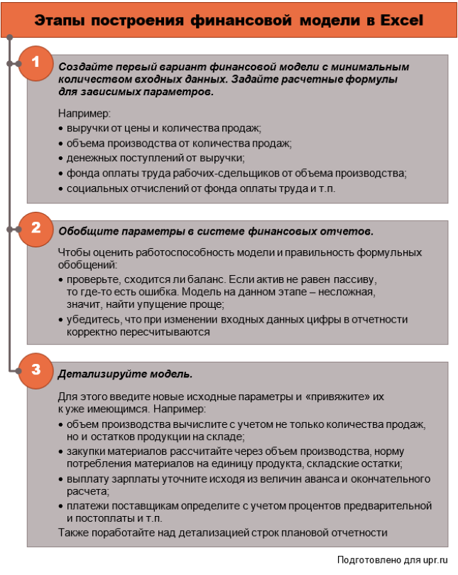
Рисунок 1. Построение финансовой модели: рекомендуемые этапы
Опробуем данный подход на практике. Рассмотрим пример для организации, которая занимается розничной торговлей. Такой выбор не случайный. Любое производство сложнее торговли, так как в нем предполагаются:
- материальные затраты;
- амортизация оборудования;
- возможно, незавершенный производственный процесс на конец месяца, поэтому необходимость разделения затрат и расходов;
- разнородные складские запасы в виде материалов и продукции.
Кроме того, продажи в розницу исключают вариант формирования дебиторской задолженности покупателей, если исходить из того, что отсрочки и рассрочки не предоставляются.
Финансовая модель (ФМ) в Excel: считаем доходы
Отправная точка на данном этапе – объем продаж. Можно пойти простым путем и внести только денежное значение выручки. Позже детализировать его как произведение цены и количества в разрезе номенклатурных позиций.
Мы сразу поступим вторым способом. Это даст количественный параметр, который необходим для корректного подсчета расходов на приобретение товаров.
Основная сложность этапа: откуда взять данные по плану продаж? Все зависит от вашей цели:
- если она пока в том, чтобы построить и «обкатать» работоспособность ФМ, то берите любые данные. Например, за прошлый год или произвольные;
- если вам одновременно нужны и модель, и качественные результаты расчета по ней, то займитесь планированием отдельно.
Мы ратуем за то, чтобы на данном этапе не уходить в детали. Но разумно уже сейчас подумать: чем будете усложнять и этим приближаться к реальности?
Вот два совета.
Первый. Покажите отдельно НДС, который «сидит» в цене реализации. Он приходит в поступлениях от покупателей, но это не доход вашей организации. Добавив его в таблицу, вы посчитаете выручку-нетто или чистый доход. Заодно определите будущие платежи в бюджет по данному налогу*.
____________________
Примечание: в бюджет платится разница между НДС, который начислен к уплате, и тем, который предъявляется к возмещению по собственным закупкам.
____________________
Второй. Введите аналитику по продажам. Самое простое – это номенклатурные позиции. Дополнительно к ним:
- процент возврата товаров;
- категория клиента (физическое лицо или организация);
- номер магазина или наименование региона, если есть несколько точек продаж.
Помним: пока излишняя детализация лишь запутает. Поэтому получаем в Excel простой план по доходам.
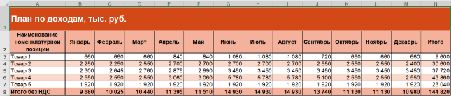
Рисунок 2. Упрощенный план по доходам в Excel
Построение финансовых моделей: пример планирования расходов
Определимся с расходами также пока в первом приближении. Обобщим полный перечень трат компании в разрезе элементов. Это будут:
- материальные траты. В упрощенном варианте предположим, что к ним относятся только траты на покупку товара без НДС и что организация продает в течение месяца столько, сколько закупает. Значит, величину определим как произведение цены приобретения и объема продаж;
- зарплата работников. Ограничимся единой суммой фонда оплаты труда за месяц без разбивки по составляющим;
- социальные отчисления. Для них составим формульную зависимость. Обычно это 30% плюс процент взносов «на травматизм» в Фонд социального страхования от начисленной оплаты труда. Данный процент зависит от класса профессионального риска по организации. Мы взяли минимальное значение 0,2%;
- амортизация. Вводим строку в ФМ, если в собственности предприятия есть основные средства и нематериальные активы. Указываем единую сумму для каждого месяца на основе средних фактических или предполагаемых значений;
- прочие расходы. Это отчасти уход в детализацию. Однако если в компании есть постоянные легко планируемые траты, то зафиксируйте их. К ним относятся: арендные платежи, траты на рекламу, на командировки и т.п.
Для упрощенной ФМ такого списка достаточно. А это четыре совета на будущее о том, чем усложнить.
Первый. Введите дополнительные позиции в материальные расходы. Например, такие:
- отопление, водоснабжение, электроэнергия;
- упаковка;
- ГСМ на автотранспорт, если он есть на балансе;
- канцелярские принадлежности и т.п.
Второй. Отдельной строкой покажите входной НДС. Когда ставка – одна (20%), то его сумма – это произведение 20% на совокупные материальные траты без НДС. Когда примешивается еще 10%, тогда:
- либо упрощайте и считайте налог по максимальной ставке;
- либо усложняйте, применяя средневзвешенное значение ставки исходя из доли в закупках с НДС по 20% и 10% в прошлые периоды.
Третий. Разделите оплату труда на составляющие:
- выделите в зарплате продавцов оклад (постоянную часть) и премию, зависящую от объема продаж (переменную компоненту);
- покажите отдельной строкой зарплату других работников, которая не завязана на количественные показатели и является постоянной.
Четвертый. Учтите изменения амортизации, если в планах организации значатся покупка или продажа основных средств и нематериальных активов.
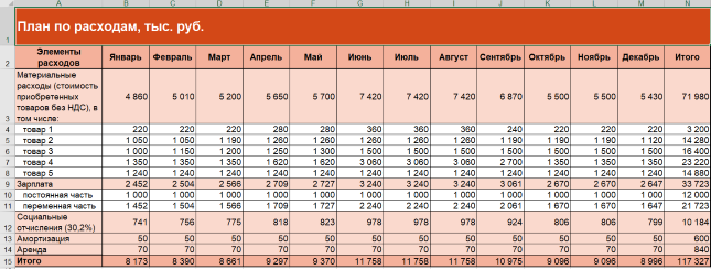
Рисунок 3. Финансовая модель бизнеса в Excel: план по расходам
То, что мы посчитали, является основой для:
- вычисления прибыли/убытка в ОФР;
- корректировки накопленного финансового результата в балансе;
- построения притоков и оттоков в ОДДС.
Перейдем ко второму этапу – обобщению данных в системе финансовых отчетов. Рассмотрим, как это делается.
Составляем плановый отчет о финансовых результатах
Формирование фактической отчетности начинается с подсчета прибыли/убытка за период. Такое же правило действует для моделей и бюджетов. Ведь чтобы заполнить раздел баланса про собственный капитал, нужна величина финансового результата.
Мы подсчитали плановые доходы и расходы по операционной деятельности. Этого достаточно, чтобы составить упрощенный отчет. Вот его возможный вариант.
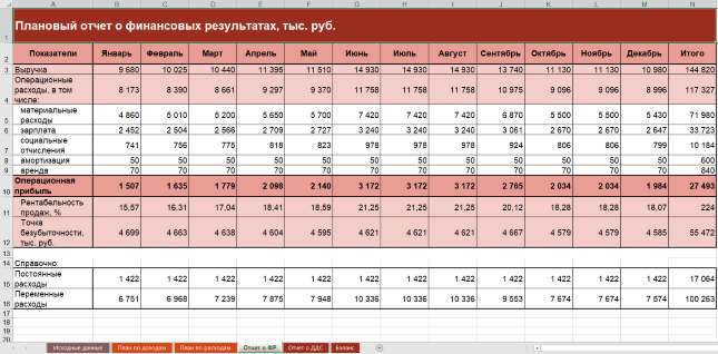
Рисунок 4. Упрощенный ОФР в Excel-модели
В нем разница между доходами и расходами показывает прибыль или убыток. Мы рассматриваем только основную деятельность без прочей. Поэтому выходим на операционный финансовый результат.
ОФР тесно связан с балансом и ОДДС. Смотрите в таблице, куда и какую информацию он передает.
Таблица 1. Взаимосвязь плановых ОФР, баланса и ОДДС
| Строка ОФР | Связанная строка баланса | Связанная строка ОДДС |
| Операционная прибыль (убыток) | Нераспределенная прибыль (убыток) – добавляется к значениям предыдущего периода | – |
| Выручка (операционные доходы) | – |
Поступления от покупателей и заказчиков – сумма выручки корректируется на авансы полученные и дебиторскую задолженность по формуле: Поступления = Выручка + Авансы полученные – Дебиторская задолженность* |
| Операционные расходы | – |
Платежи по текущей деятельности – сумма денежных** расходов корректируется на авансы выданные и кредиторскую задолженность по формуле: Платежи = Денежные расходы + Авансы выданные – Кредиторская задолженность |
|
Примечание: * в примере ФМ формируется по организации розничной торговли. Поэтому полагаем: авансов и дебиторки от покупателей нет. Значит, поступления равняются выручке; ** денежные расходы – те, которые приводят к оттоку денег (зарплата, налоги, материальные). Для сравнения: к неденежным относится амортизация |
Чтобы плановый ОФР оказался более информативным, дополним строками:
- рентабельность продаж. Это расчетный показатель, который равняется отношению прибыли (в данном случае – операционной) к выручке;
- точка безубыточности в денежном выражении. Для ее расчета предварительно разделили расходы на постоянные и переменные. Об особенностях классификации затрат по такому принципу читайте в статье «Расчет себестоимости».
Формируем плановый отчет о движении денежных средств
Здесь задача:
- обобщить денежные притоки и оттоки;
- рассчитать чистый денежный поток как разницу между ними;
- прибавить его значение к остатку денег на начало периода и вычислить остаток денег на конец. Через эту сумму ОДДС связан с балансом.
Для создаваемой ФМ исходим из допущений:
- организация занимается только основной деятельностью. При этом не покупает оборудование и ценные бумаги, не берет и не дает взаймы, не принимает новых учредителей. Значит, формируется один вид денежных операций – текущий. О двух других – инвестиционных и финансовых – читайте в статье «Анализ движения денежных средств компании»;
- товары оплачиваются поставщику двумя платежами: 60% – аванс в месяце, который предшествует поставке, 40% – окончательный расчет сразу после принятия на склад;
- зарплата выплачивается двумя переводами: 50% – аванс в месяце начисления, 50% – перевод остатка в периоде, который следует за отработанным;
- страховые взносы перечисляются в месяце, идущем за их начислением;
- прочая составляющая расходов по обычным видам деятельности представлена арендой. Платежи по ней производятся в месяце начисления арендной платы.
Получаем вариант ОДДС.
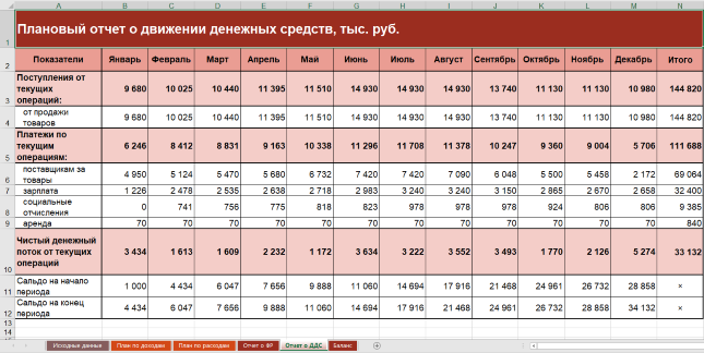
Рисунок 5. Упрощенный отчет о движении денежных средств в ФМ
Сводим плановый баланс
Предположим, что у организации:
- нет входящих остатков по запасам, дебиторской и кредиторской задолженности;
- имущество включает одно основное средство и деньги;
- в пассиве – только уставный капитал и нераспределенная прибыль.
Схема заполнения балансовых строк окажется следующей.
Таблица 2. Техника сведения упрощенного баланса
| Показатель на начало месяца | Расчетная формула | Пояснения |
| Основные средства | Основные средства на начало предыдущего месяца (баланс) – Амортизация за месяц (ОФР) | – |
| Запасы | – | Неизменны и равняются нулю из-за допущения: закупаемые товары полностью распродаются в течение месяца |
| Дебиторская задолженность | Дебиторская задолженность на начало предыдущего месяца (баланс) + Платежи поставщикам за товары (ОДДС) – Материальные расходы (ОФР) | В примере нет дебиторки покупателей, так как организация торгует в розницу |
| Денежные средства | Денежные средства на начало предыдущего месяца (баланс) + Чистый денежный поток за месяц (ОДДС) | – |
| Уставный капитал | – | Неизменен и равняется 1000 тыс. руб. из-за допущения: новых учредителей в течение года не было |
| Нераспределенная прибыль | Нераспределенная прибыль на начало предыдущего месяца (баланс) + Прибыль за месяц (ОФР) | – |
| Кредиторская задолженность | Кредиторская задолженность на начало предыдущего месяца + Начисления по зарплате, социальным отчислениям и аренде (ОФР) – Платежи по зарплате, социальным отчислениям и аренде (ОДДС) | – |
Формат баланса будет таким.
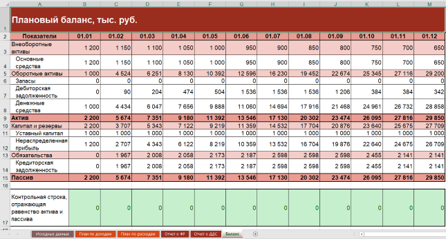
Рисунок 6. Упрощенный баланс в финансовой модели в Excel
Детализация финансовой модели в Excel
О возможных вариантах усложнения исходных данных рассказывали выше. Здесь остановимся на детализации строк плановой отчетности. Вот несколько советов:
- используйте разные группировки расходов в ОФР. Мы обобщили их по элементам. Такой подход называется «по характеру расходов». Но он – не единственный. Можно одновременно с ним или вместо него использовать функциональную классификацию с выделением себестоимости продаж, а также расходов на сбыт и управление. Подробнее про такие варианты читайте в статье «БДР: бюджет доходов и расходов»;
- добавьте другие виды прибыли в ОФР. Например, валовую. Она покажет разницу между продажной и закупочной ценами товаров. Если в организации есть прочие операции, то в отчете не обойтись без чистой прибыли. Читайте о видах финансового результата в материале «Анализ финансовых результатов деятельности компании»;
- включите в ОФР строки для прочих доходов и расходов. Растущая организация не сможет обходиться без них. Например, взятие кредита приведет к появлению процентных платежей по нему. Они – это прочий расход;
- расширьте ОДДС за счет инвестиционных и финансовых операций, если собираетесь приобретать оборудование и брать взаймы. Не смешивайте такие денежные потоки с текущими;
- детализируйте сложносоставные строки в балансе. Например, из запасов выделите товары, материалы, готовую продукцию и незавершенное производство (последние два пункта – неактуальны для торговли). Из состава дебиторки: авансы выданные поставщикам и долги покупателей. По аналогии поступите с кредиторкой и покажите в отдельных статьях: авансы полученные, задолженность перед поставщиками, перед персоналом по оплате труда, по налогам и страховым взносам, перед учредителями по дивидендам.
Не забудьте скачать Excel-файл с полученной финансовой моделью из начала статьи.
Финансовое моделирование в Excel помогает понять:
- как планируемые руководством мероприятия отразятся на величине имущества, капитала, обязательств, доходов, расходов и прибыли;
- какие факторы больше других влияют на прибыль, ликвидность и финансовую устойчивость организации.
Важна роль ФМ и в план-фактном анализе. В течение отчетного периода сравнивайте ожидания из нее с тем, как получилось в реальности. Это хороший способ контролировать ситуацию: понимать суть нарождающихся тенденций и того, к чему они приведут бизнес.