
Excel для Microsoft 365 Excel для Microsoft 365 для Mac Excel для Интернета Excel 2021 Excel 2021 для Mac Excel 2019 Excel 2019 для Mac Excel 2016 Excel 2016 для Mac Excel 2013 Excel 2010 Excel 2007 Excel для Mac 2011 Excel Starter 2010 Еще…Меньше
В этой статье описаны синтаксис формулы и использование функции COS в Microsoft Excel.
Описание
Возвращает косинус заданного угла.
Синтаксис
COS(число)
Аргументы функции COS описаны ниже.
-
Число — обязательный аргумент. Угол в радианах, для которого определяется косинус.
Замечания
Если угол задан в градусах, умножьте его на ПИ()/180 или воспользуйтесь функцией РАДИАНЫ, чтобы преобразовать его в радианы.
Пример
Скопируйте образец данных из следующей таблицы и вставьте их в ячейку A1 нового листа Excel. Чтобы отобразить результаты формул, выделите их и нажмите клавишу F2, а затем — клавишу ВВОД. При необходимости измените ширину столбцов, чтобы видеть все данные.
|
Формула |
Описание |
Результат |
|
=COS(1,047) |
Косинус 1,047 радиан |
0,5001711 |
|
=COS(60*ПИ()/180) |
Косинус 60 градусов |
0,5 |
|
=COS(РАДИАНЫ(60)) |
Косинус 60 градусов |
0,5 |
Нужна дополнительная помощь?
Excel for Microsoft 365 Excel for Microsoft 365 for Mac Excel for the web Excel 2021 Excel 2021 for Mac Excel 2019 Excel 2019 for Mac Excel 2016 Excel 2016 for Mac Excel 2013 Excel 2010 Excel 2007 Excel for Mac 2011 Excel Starter 2010 More…Less
This article describes the formula syntax and usage of the COS function in Microsoft Excel.
Description
Returns the cosine of the given angle.
Syntax
COS(number)
The COS function syntax has the following arguments:
-
Number Required. The angle in radians for which you want the cosine.
Remark
If the angle is in degrees, either multiply the angle by PI()/180 or use the RADIANS function to convert the angle to radians.
Example
Copy the example data in the following table, and paste it in cell A1 of a new Excel worksheet. For formulas to show results, select them, press F2, and then press Enter. If you need to, you can adjust the column widths to see all the data.
|
Formula |
Description |
Result |
|
=COS(1.047) |
Cosine of 1.047 radians |
0.5001711 |
|
=COS(60*PI()/180) |
Cosine of 60 degrees |
0.5 |
|
=COS(RADIANS(60)) |
Cosine of 60 degrees |
0.5 |
Need more help?
Want more options?
Explore subscription benefits, browse training courses, learn how to secure your device, and more.
Communities help you ask and answer questions, give feedback, and hear from experts with rich knowledge.
Функция SIN в Excel используется для вычисления синуса угла, заданного в радианах, и возвращает соответствующее значение.
Функция SINH в Excel возвращает значение гиперболического синуса заданного вещественного числа.
Функция COS в Excel вычисляет косинус угла, заданного в радианах, и возвращает соответствующее значение.
Функция COSH возвращает значение гиперболического косинуса заданного вещественного числа.
Примеры использования функций SIN, SINH, COS и COSH в Excel
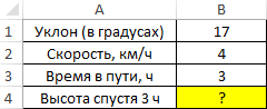
Пример 1. Путешественник движется вверх на гору с уклоном в 17°. Скорость движения постоянная и составляет 4 км/ч. Определить, на какой высоте относительно начальной точке отсчета он окажется спустя 3 часа.
Таблица данных:
Для решения используем формулу:
=B2*B3*SIN(РАДИАНЫ(B1))
Описание аргументов:
- B2*B3 – произведение скорости на время пути, результатом которого является пройденное расстояние (гипотенуза прямоугольного треугольника);
- SIN(РАДИАНЫ(B1)) – синус угла уклона, выраженного в радианах с помощью функции РАДИАНЫ.
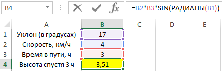
В результате расчетов мы получили величину малого катета прямоугольного треугольника, который характеризует высоту подъема путешественника.
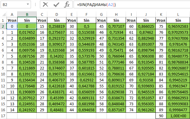
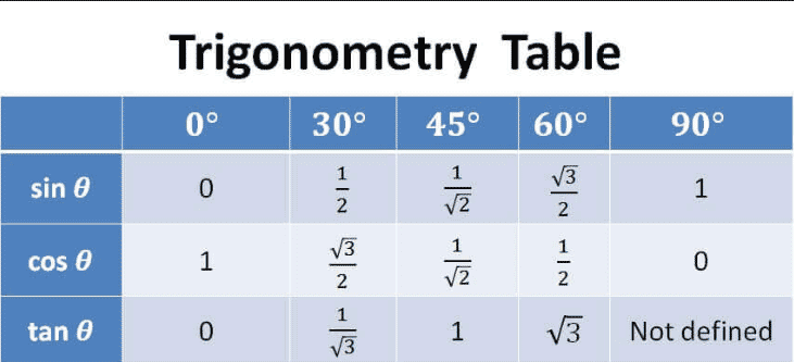
Таблица синусов и косинусов в Excel
Пример 2. Ранее в учебных заведениях широко использовались справочники тригонометрических функций. Как можно создать свой простой справочник с помощью Excel для косинусов углов от 0 до 90?
Заполним столбцы значениями углов в градусах:
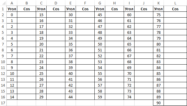
Для заполнения используем функцию COS как формулу массива. Пример заполнения первого столбца:
=COS(РАДИАНЫ(A2:A16))
Вычислим значения для всех значений углов. Полученный результат:
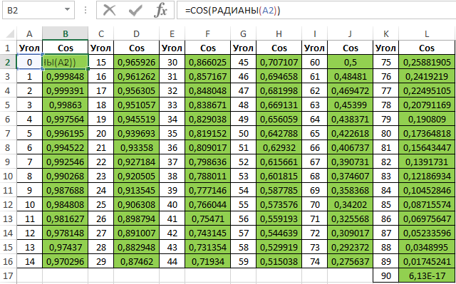
Примечание: известно, что cos(90°)=0, однако функция РАДИАНЫ(90) определяет значение радианов угла с некоторой погрешностью, поэтому для угла 90° было получено отличное от нуля значение.
Аналогичным способом создадим таблицу синусов в Excel:
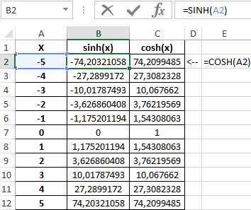
Построение графика функций SINH и COSH в Excel
Пример 3. Построить графики функций sinh(x) и cosh(x) для одинаковых значений независимой переменной и сравнить их.
Исходные данные:
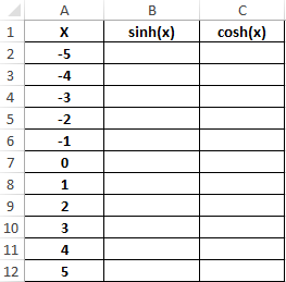
Формула для нахождения синусов гиперболических:
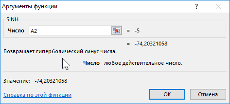
=SINH(A2:A12)
Формула для нахождения косинусов гиперболических:
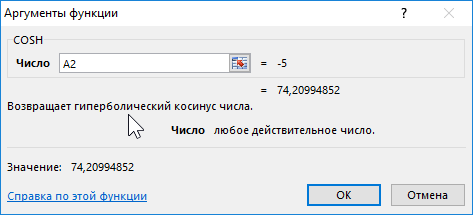
=COSH(A2:A12)
Таблица полученных значений:
Построим графики обеих функций на основе имеющихся данных. Выделите диапазон ячеек A1:C12 и выберите инструмент «ВСТАВКА»-«Диаграммы»-«Вставь точечную (X,Y) или пузырьковую диаграмму»-«Точечная с гладкими кривыми и маркерами»:
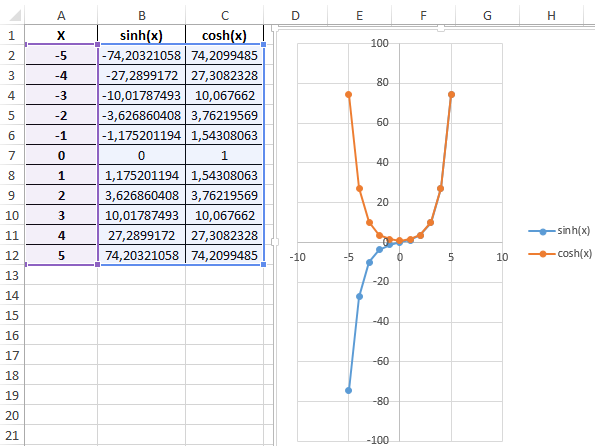
Как видно, графики совпадают на промежутке (0;+∞), а в области отрицательных значений x части графиков являются зеркальными отражениями друг друга.
Особенности использования тригонометрических функций в Excel
Синтаксис функции SIN:
=SIN(число)
Синтаксис функции SINH:
=SINH(число)
Синтаксис функции COS:
=COS(число)
Синтаксис функции COSH:
>=COSH(число)
Каждая из приведенных выше функций принимает единственный аргумент число, который характеризует угол, заданный в радианах (для SIN и COS) или любое значение из диапазона вещественных чисел, для которого требуется определить гиперболические синус или косинус (для SINH и COSH соответственно).
Примечания 1:
- Если в качестве аргумента любой из рассматриваемых функций были переданы текстовые данные, которые не могут быть преобразованы в числовое значение, результатом выполнения функций будет код ошибки #ЗНАЧ!. Например, функция =SIN(“1”) вернет результат 0,8415, поскольку Excel выполняет преобразование данных там, где это возможно.
- В качестве аргументов рассматриваемых функций могут быть переданы логические значения ИСТИНА и ЛОЖЬ, которые будут интерпретированы как числовые значения 1 и 0 соответственно.
- Все рассматриваемые функции могут быть использованы в качестве формул массива.
Примечения 2:
- Синус гиперболический рассчитывается по формуле: sinh(x)=0,5*(ex-e-x).
- Формула расчета косинуса гиперболического имеет вид: cosh(x)=0,5*( ex+e-x).
- При расчетах синусов и косинусов углов с использованием формул SIN и COS необходимо использовать радианные меры углов. Если угол указан в градусах, для перевода в радианную меру угла можно использовать два способа:
Скачать примеры тригонометрических функций SIN и COS
- Функция РАДИАНЫ (например, =SIN(РАДИАНЫ(30)) вернет результат 0,5;
- Выражение ПИ()*угол_в_градусах/180.

This Excel tutorial explains how to use the Excel COS function with syntax and examples.
Description
The Microsoft Excel COS function returns the cosine of an angle.
The COS function is a built-in function in Excel that is categorized as a Math/Trig Function. It can be used as a worksheet function (WS) and a VBA function (VBA) in Excel. As a worksheet function, the COS function can be entered as part of a formula in a cell of a worksheet. As a VBA function, you can use this function in macro code that is entered through the Microsoft Visual Basic Editor.
Syntax
The syntax for the COS function in Microsoft Excel is:
COS( number )
Parameters or Arguments
- number
- A numeric value used to calculate the cosine.
Returns
The COS function returns a numeric value.
Applies To
- Excel for Office 365, Excel 2019, Excel 2016, Excel 2013, Excel 2011 for Mac, Excel 2010, Excel 2007, Excel 2003, Excel XP, Excel 2000
Type of Function
- Worksheet function (WS)
- VBA function (VBA)
Example (as Worksheet Function)
Let’s look at some Excel COS function examples and explore how to use the COS function as a worksheet function in Microsoft Excel:
Based on the Excel spreadsheet above, the following COS examples would return:
=COS(A1)
Result: 0.980066578

=COS(A2)
Result: 0.939372713

=COS(A3)
Result: -0.999964658

=COS(200)
Result: 0.487187675
Example (as VBA Function)
The COS function can also be used in VBA code in Microsoft Excel.
Let’s look at some Excel COS function examples and explore how to use the COS function in Excel VBA code:
Dim LNumber As Double

LNumber = Cos(210)
In this example, the variable called LNumber would now contain the value of -0.883877473.
COS Excel function is an inbuilt trigonometric function. It is used to calculate the cosine value of a given number or, in terms of trigonometry, the cosine value of a given angle. Here, the angle is a number in Excel. This function takes only a single argument which is the input number provided.
It is a built-in function in MS Excel. It is categorized under Math functions in MS Excel. The function returns the cosine of an angle given in radians. The parameter is the value of the angle for which the cosine is to be calculated. The angle can be calculated using the RADIANS function or multiplying by PI()/180.
Table of contents
- COS Excel Function
- COS Formula
- How to Use COS Function in Excel?
- Example #1 – Calculate the value of cos (0)
- Example #2 – Calculate the value of cos (30)
- Example #3 – Calculate the value of cos (45)
- Example #4 – Calculate the value of cos (60)
- Example# 5 – Calculate the value of cos (90)
- Things to remember about the COS Function in Excel
- Usage of COS function in Excel VBA
- VBA Example #1
- VBA Example# 2
- Recommended Articles
COS Formula
The COS Formula in Excel is as follows:

The COS formula in Excel has one argument, which is a required parameter.
- number = This is a required parameter. It indicates the angle for which the cosine is to be calculated.
How to Use COS Function in Excel?
The COS can be used in Excel worksheets as a Worksheet (WS) function and Excel VBA. As a WS function, it can be entered as a part of the COS formula in a worksheet cell. As a VBA functionVBA functions serve the primary purpose to carry out specific calculations and to return a value. Therefore, in VBA, we use syntax to specify the parameters and data type while defining the function. Such functions are called user-defined functions.read more, it can be entered into the VBA code.
You can download this COS Function Excel Template here – COS Function Excel Template
Refer to the examples given below to understand better.
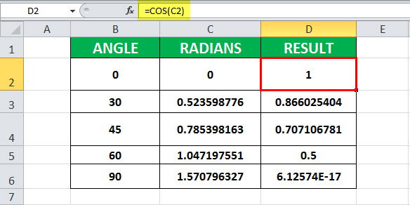
Example #1 – Calculate the value of cos (0)

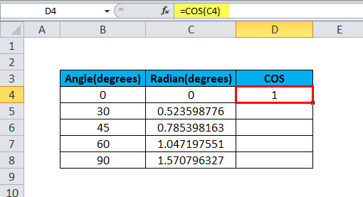
In this example, cell B2 contains the value of the angle for which cosine is to be calculated. Cell C2 has a COS formula associated with it, which is RADIANS. COS in excel is assigned to cell D2. RADIANS(B2) is 0. Further, COS is applied to 0, which is 1.
Hence, the resultant cell D2 has a value of 1 as COS(0) is 1.
Example #2 – Calculate the value of cos (30)
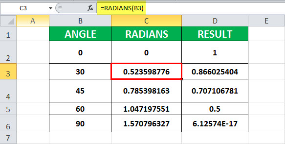
In this example, cell B3 contains the value of the angle for which cosine is to be calculated. Cell C3 has a COS formula associated with it, which is RADIANS. COS in excel is assigned to the D3 cell. RADIANS(B3) is 0.523598776. Further, COS is applied to 0.523598776, which is 0.866025404.
Hence, the resultant cell D3 has a value of 1 as COS (0.523598776) is 1.

Example #3 – Calculate the value of cos (45)

In this example, cell B4 contains the value of the angle for which cosine is to be calculated. Cell C4 has a COS formula associated with it, which is RADIANS. COS is assigned to the D4 cell. RADIANS(B3) is 0.523598776. Further, COS is applied to 0.785398163, which is 0.707106781.
Hence, the resultant cell D4 has the value of 1 as COS (0.707106781) is 1.

Example #4 – Calculate the value of cos (60)

In this example, cell B5 contains the value of the angle for which cosine is to be calculated. Cell C5 has a COS formula associated with it, which is RADIANS. COS is assigned to the D5 cell. RADIANS(B5) is 1.047197551. Further, COS is applied to 1.047197551, which is 0.5.
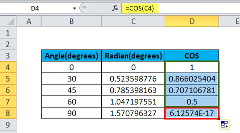
Hence, the resultant cell D5 has a value of 0.5 as COS (1.047197551) is 0.5.

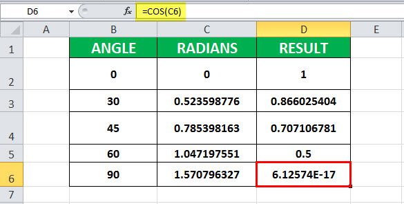
Example# 5 – Calculate the value of cos (90)

In this example, cell B6 contains the value of the angle for which cosine is to be calculated. Cell C6 has a COS formula associated with it, which is B6*PI ()/180. COS is assigned to the D6 cell. 90*PI ()/180 is 1.570796327. The value of PI () is 3.14159. So, it is 90 * (3.14159/180) =1.570796327. Further, COS is applied to 1.570796327, which is 6.12574E-17.
Hence, the resultant cell D6 has 6.12574E-17, as COS (1.570796327) is 6.12574E-17.
Things to remember about the COS Function in Excel
- The COS in Excel always expects radians as the parameter for which the cosine is calculated.
- If the angle is in degrees, it must be calculated using the RADIANS function or multiply the angle by PI ()/180.
Usage of COS function in Excel VBA
The COS in Excel can be used in Excel VBA as follows. First, it serves the same purpose: to get the cosine value of the angle provided.
Syntax: COS ( Number )
VBA Example #1
Dim val1 As Double

val1 = Cos ( 0 )

val1 : 1
Here, val1 is a variable. It is declared as Double, which indicates it can hold data with the double data type. The cosine of 0 is 1. Hence, val1 has value 1.
VBA Example# 2
Const pi = 3.1415
Dim val As Double

' Convert 45 degrees to radians by multiplying by pi/180.
val = Cos (45 * pi / 180 )
' The variable val is now  equal to 0.7071067
Here, angle 45 is converted to radians using the same COS formula in the Excel worksheet.
If a non-numeric value is provided to the Cos in Excel, it will return a
If a non-numeric value is provided to the Cos in excel then, it will return Type MismatchWhen we assign a value to a variable that is not of its data type, we get Type mismatch Error or Error code 13. For example, if we assign a decimal or long value to an integer data type variable, we will get this error (Error Code 13) when we run the code.read more error in Excel VBA code.
Recommended Articles
This article has been a guide to COS Function in Excel. Here, we discuss the COS formula in Excel and how to use it, Excel examples, and downloadable Excel templates. You may also look at these useful functions in Excel: –
- SIGN Function
- AVERAGE Function in Excel
- Excel TAN Function
- LN Excel Function | Examples
- Excel DSUM
This article describes the formula syntax and usage of the COS function in Microsoft Excel.
Example.
| Formula | Description | Result |
|---|---|---|
| =COS(60*PI()/180) | Cosine of 60 degrees | 0.5 |
| =COS(RADIANS(60)) | Cosine of 60 degrees | 0.5 |
Contents
- 1 How do you put COS 1 in Excel?
- 2 What is the use of COS function?
- 3 How do you put degrees in Excel?
- 4 What is pi on Excel?
- 5 How do I know if I have SOH CAH TOA?
- 6 How do you write a cosine function?
- 7 What is COSX equal to?
- 8 What is the value of cosine?
- 9 How do I insert a degree symbol?
- 10 How do you write 90 degrees in Excel?
- 11 How do I make the degree symbol?
- 12 How do you add pi in Excel?
- 13 How do you find pi data in Excel?
- 14 How do you use pi formula?
- 15 What is Sohcahtoa used for?
- 16 Is Sohcahtoa a trigonometry?
- 17 How do you write a period with amplitude and cosine?
- 18 Is Cos an even function?
- 19 How do you integrate 1 cosine?
- 20 Can Cos equal 1?
How do you put COS 1 in Excel?
Excel ACOS Function
- Summary. The ACOS function returns the inverse cosine of a number.
- Get the inverse cosine of a value, in radians.
- Angle in radians.
- =ACOS (number)
- number – The value to get the inverse cosine of. The number must be between -1 and 1 inclusive.
- The ACOS function returns the inverse cosine of a value.
What is the use of COS function?
The cosine function is a periodic function which is very important in trigonometry. The simplest way to understand the cosine function is to use the unit circle. For a given angle measure θ , draw a unit circle on the coordinate plane and draw the angle centered at the origin, with one side as the positive x -axis.
How do you put degrees in Excel?
Method #1: Use the symbol library to get the degree symbol
- In a cell, type ‘180’ (without the quotes).
- Then go to Insert tab and click the Symbol icon (far right).
- In the dropdown box at the top, select the Symbol font.
- Scroll down and select the degree symbol.
- Click Insert.
What is pi on Excel?
The PI Function in Excel returns the mathematical constant “pi.” To recap, PI is the ratio of a circle’s circumference and its diameter. Often, we would use the PI Function in Excel, especially when our business is required to do geometric calculations.
How do I know if I have SOH CAH TOA?
In this geometry lesson, you’re going to learn all about SohCahToa. It’s probably one of the most famous math mnemonics alongside PEMDAS.
It’s defined as:
- SOH: Sin(θ) = Opposite / Hypotenuse.
- CAH: Cos(θ) = Adjacent / Hypotenuse.
- TOA: Tan(θ) = Opposite / Adjacent.
How do you write a cosine function?
Any cosine function can be written as a sine function. y = A sin(Bx) and y = A cos(Bx). The number, A, in front of sine or cosine changes the height of the graph. The value A (in front of sin or cos) affects the amplitude (height).
What is COSX equal to?
Remember the Pythagorean triple 8, 15, 17? The reference triangle has horizontal leg 8, vertical leg 15, hypotenuse 17…so cos x = 8/17. Another way to do this is to recall that 1 + tan2x = sec2x & secant is reciprocal of cosine.
What is the value of cosine?
0
As can be seen from the figure, cosine has a value of 0 at 90° and a value of 1 at 0°. Sine follows the opposite pattern; this is because sine and cosine are cofunctions (described later). The other commonly used angles are 30° ( ), 45° ( ), 60° ( ) and their respective multiples.
How do I insert a degree symbol?
How to type the degree symbol on an Android
- Tap a place that you’re able to type so the keyboard appears.
- Tap the ? 123 icon in the bottom-left corner, and then the =< icon above it.
- The degree symbol will be on this page. Tap it to type it.
How do you write 90 degrees in Excel?
Right-click and then select “Format Cells” from the popup menu. When the Format Cells window appears, select the Alignment tab. Then set the number of degrees that you wish to rotate the text. This value ranges from 90 degrees to -90 degrees for Orientation.
How do I make the degree symbol?
If you are using Excel, you can add a degree symbol by typing “=CHAR(176)” in a cell. Press and hold Alt and type 0176 on Windows with a numeric keypad.
How do you add pi in Excel?
How to Use PI in Excel
- Open your Excel spreadsheet and type “=” into a blank cell to label its contents as a mathematical formula.
- Type “PI()”, which is equivalent to “3.14159265358979” in an Excel formula.
- Type the remainder of your formula.
- Press “Enter” to run the formula.
How do you find pi data in Excel?
Procedure
- Go to the Data tab and click Get External Data > From Other Sources > From Data Connection Wizard.
- In the Data Connection Wizard dialog, select the Other/advanced item and click Next.
- Configure a Universal Data Link (UDL) to a PI Server.
- Select the database that contains the data you want.
How do you use pi formula?
Use the formula.
The circumference of a circle is found with the formula C= π*d = 2*π*r. Thus, pi equals a circle’s circumference divided by its diameter. Plug your numbers into a calculator: the result should be roughly 3.14.
What is Sohcahtoa used for?
SOHCAHTOA is a mnemonic device helpful for remembering what ratio goes with which function. With these properties, you can solve almost any problem related to finding either a side length or angle measure of a right triangle. SohCahToa can ensure that you won’t get them wrong.
Is Sohcahtoa a trigonometry?
Sohcahtoa: SOHCAHTOA is a mnemonic device that is used in mathematics to remember the definitions of the three most common trigonometric functions.Sine, cosine, and tangent are the three main functions in trigonometry. They’re all based on ratios obtained from a right triangle.
How do you write a period with amplitude and cosine?
1 Answer
- In y=acos(b(x−c))+d :
- • |a| is the amplitude. • 2πb is the period.
- The amplitude is 3 , so a=3 .
- The period is 2π3 , so we solve for b .
- b=3.
- The phase shift is +π9 , so c=π9 .
- The vertical transformation is +4 , so d=4 .
- ∴ The equation is y=3cos(3(x−π9))+4 , which can be written as y=3cos(3x−π3)+4.
Is Cos an even function?
Sine is an odd function, and cosine is an even function. You may not have come across these adjectives “odd” and “even” when applied to functions, but it’s important to know them. A function f is said to be an odd function if for any number x, f(–x) = –f(x).
How do you integrate 1 cosine?
∫ (1 / cos(x)) dx = ∫ sec(x) dx = ln |sec(x) + tan(x)| + C, where C is a constant. The antiderivative of 1 / cos(x) is ln |sec(x) + tan(x)| + C, where C is a constant.
Can Cos equal 1?
1 Expert Answer
1) In the unit circle the x represent the cosine of the function and the y represent the sine of the trigonometric function. 2) Looking at the unit circle I noticed that cos(x) =1, corresponds to 360°. in other words cos (360º) =1, the answer is x=360º or x=2π radians.
Summary
The Excel COS function returns the cosine of an angle given in radians. To supply an angle to COS in degrees, use the RADIANS function to convert to radians.
Purpose
Get the cosine of an angle provided in radians.
Return value
Arguments
- number — The angle in radians for which you want the cosine.
Syntax
Usage notes
The COS function returns the cosine of an angle provided in radians. In geometric terms, the cosine of an angle returns the ratio of a right triangle’s adjacent side over its hypotenuse. For example, the cosine of PI()/6 radians (30°) returns the ratio 0.866.
=COS(PI()/6) // Returns 0.886
Using Degrees
To supply an angle to COS in degrees, multiply the angle by PI()/180 or use the RADIANS function to convert to radians. For example, to get the COS of 60 degrees, you can use either formula below:
=COS(60*PI()/180)
=COS(RADIANS(60))
Explanation

The graph of cosine above visualizes the output of the function for all angles from 0 to a full rotation. Geometrically, the function returns the x-component of the point corresponding to an angle on the unit circle. Since the cosine of an angle returns a ratio, the output of the function will always be in the range [-1, 1].
Graph courtesy of wumbo.net

Author![]()
Dave Bruns
Hi — I’m Dave Bruns, and I run Exceljet with my wife, Lisa. Our goal is to help you work faster in Excel. We create short videos, and clear examples of formulas, functions, pivot tables, conditional formatting, and charts.
Great site — amazingly clear but with a lot of depth in terms of the explanations.
Get Training
Quick, clean, and to the point training
Learn Excel with high quality video training. Our videos are quick, clean, and to the point, so you can learn Excel in less time, and easily review key topics when needed. Each video comes with its own practice worksheet.
View Paid Training & Bundles
Help us improve Exceljet
COS Function (Table of Content)
- COS in Excel
- How to Use COS Function?
Excel COS Function
Cos function in excel is a mathematical function that calculates the Cos value of any angle. As we know, Cos angle is the ratio of Base to Hypotenuse, but in excel, we need to select radians function here along with COS Function to get the proper angle value. Also, we can multiply the input angel value with Pi()/180 other than using the Radians function.
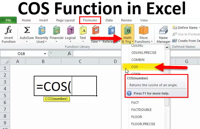
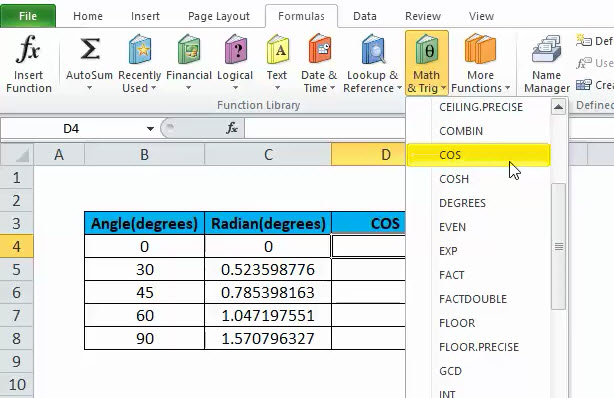
It comes under head Formulas and the Math & Trig. The screenshot is given below:
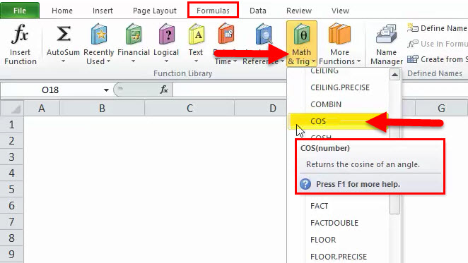
We can see in the above pic that the COS is the formula for trigonometry in Mathematics. This function is built of MS Excel. The function of the COS is that it returns the cosine of a given angle in radians. We can calculate the angle by using the RADIANS function, or we can multiply it by PI()/180. It can be used as a worksheet function (WS) and VBA function, and Microsoft Excel. If we are using it in the worksheet function, we can enter the formula in a cell of a worksheet, and if we are using it through VBA, it should be entered as macro code in Microsoft Visual Basic Editor.
COS Formula in Excel:
Below is the COS Formula.
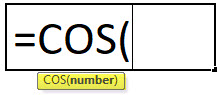
This formula has one argument, which is number, and it is the mandatory parameter.
Number: this is the which shows the angle for which the calculation of cosine is going to occur.
We can also use this formula just entering into one cell as =COS(number) in Microsoft Excel.
How COS Function Works?
As we know, Trigonometry is a branch of mathematics in which we study about the relations between the elements of a triangle which is as sides and angles. Microsoft Excel has lots of Trigonometry function which is inbuilt, to help complex problems of the same. The user has to keep in mind while solving or using these functions that Microsoft Excel performs the result or calculation considering angle value in radians but not in degrees, which makes the process different from doing it manually.
For example, we know that COS 30 = 0.866, but when we enter directly, it will result as 0.154, so we have to convert in radians and then calculate the COS on radians.
How to Use the COS Function in Excel?
This COS Function is very easy to use. Let us now see how to use the COS function in Excel with the help of some examples.
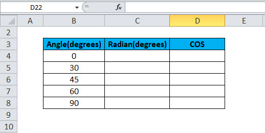
Example #1
As we discussed, first, we need to calculate the Radians for the given angle, and then we will calculate the COS.
Step 1: First, we will take the raw data for which COS needs to be calculated. Below is the picture:
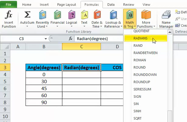
Step 2: Now, we have to click on Formulas and under that Math & Trig. We can see this step in below pic:
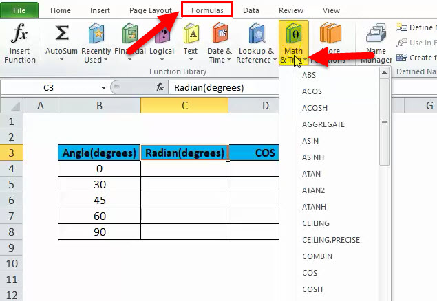
So, we can see that there are lots of functions listed in this category.
Step 3: Now, we have to go on option Radian and click it. We can see this step in below pic:
Step 4: Now, we have to select B4 as an angle to achieve the result and then click Enter. Please refer to the below pic:
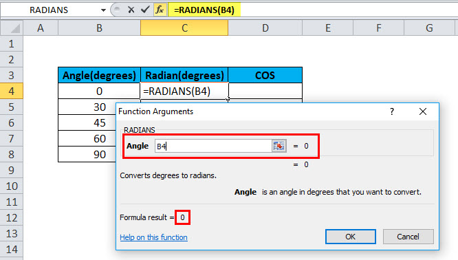
After pressing Enter, the result will be shown like below:
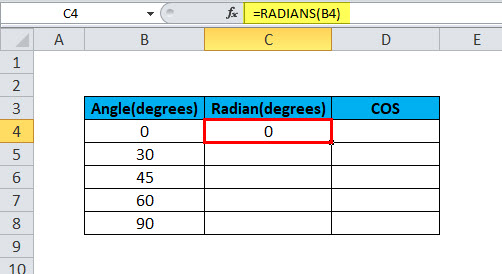
Step 5: Now, we can drag the formula to each degree, like shown in the below screenshot.
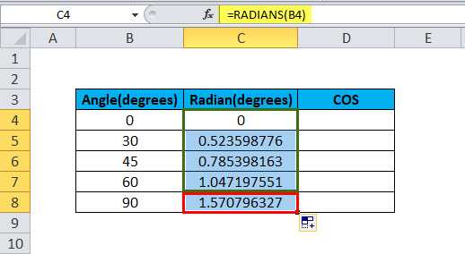
So, we have the Radians ready; now, we have to calculate the COS for these Radians.
Step 6: We have to repeat step 1 & step 2 and select the COS option. Below is the picture for reference.
Step 7: Now, we have to click on COS, select the C4, and press Enter or click OK.
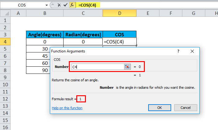
After clicking OK, we have the below result:
Step 8: We can drag the formula for D5 to D8, and we will have the result.
So, we have the results ready. We understood from the above step that firstly, RADIANS need to be calculated before calculating COS. After calculating RADIANS, we have to calculate the COS on that RADIANS, and it will give the desired result, which will be COSINE for each angle.
Example #2
As we discussed earlier, we can use it in the VBA code as well as in Microsoft Excel. So, below is one of the codings to use the COS function as a VBA code.
Dim LNumber As Double
LNumber = COS(5)
The Lnumber above is 0.523598776, which is as a variable.
Example #3
We will see in VBA to apply on degree 30.
So, below is the solution:
Dim val As Double
‘Convert 30 degrees to RADIANS by multiplying by PI/180.
Val = COS(30*PI/180)
‘The variable value is now equal to 0.86602.
So, in the above formula, angle 30 is converted into radians first and then COS.
Things to Remember
- If the angle is given in degrees for which we have to calculate COS, we have to calculate RADIANS for the same, or we can multiply the angle by PI()/180.
- COS always uses the parameter as RADIANS.
Recommended Articles
This has been a guide to COS Function. Here we discuss the COS Formula and how to use the COS function along with practical examples and downloadable excel templates. You can also go through our other suggested articles –
- Excel XIRR Function
- Excel SIN Function
- EOMONTH Function Excel
- Excel DEGREES Function
This post will guide you how to use Excel COS function with syntax and examples in Microsoft excel.
Description
The Excel COS function returns the cosine of a given angle. If you want to supply an angle to COS function in degrees, then you need to multiply the angle by PI()/180. Or you can use the RADIANS function to the angle to radians.
The COS function is a build-in function in Microsoft Excel and it is categorized as a Math and Trigonometry Function.
The COS function is available in Excel 2016, Excel 2013, Excel 2010, Excel 2007, Excel 2003, Excel XP, Excel 2000, Excel 2011 for Mac.
Syntax
The syntax of the COS function is as below:
= COS(number)
Where the COS function argument is:
- number –This is a required argument. A number that used to be calculate the cosine of an angle.
Note:
- If your argument is in degrees, multiply it by PI()/180 or use the RADIANS function to convert it to radians.
Excel COS Function Examples
The below examples will show you how to use Excel COS Function to return the cosine of an angle.
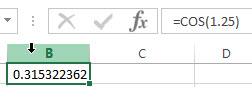
1# get the cosine of 1.25 radians, enter the following formula in Cell B1.
=COS(1.25)
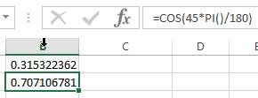
2# get the cosine of 45 degrees, enter the following formula in Cell B2.
=COS(45*PI()/180)
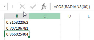
3# get the cosine of 30 degrees, enter the following formula in Cell B3.
=COS(RADIANS(30))
- Excel SIN function
The Excel TANH function returns the hyperbolic tangent of a given number.The syntax of the TANH function is as below:=TANH (number)… - Excel ACOS function
The Excel ACOS function returns the arccosine value of a number.The ACOS function is a build-in function in Microsoft Excel and it is categorized as a Math and Trigonometry Function.The syntax of the ACOS function is as below:= ACOS(number)… - Excel ACOSH function
The Excel ACOSH function returns the inverse hyperbolic cosine of a number.The syntax of the ACOSH function is as below:= ACOSH (number)… - Excel ASIN function
The Excel ASIN function returns the arcsine value of a number.The syntax of the ASIN function is as below:= ASIN (number)… - Excel PI function
The Excel PI function returns the value of mathematical constant PI. The returned value is 3.14159265358979 and ti will accurate to 15 digits.The syntax of the PI function is as below:=PI()… - Excel TAN function
The Excel TAN function returns the tangent of a given angle. So you can use this function to calculate the tangent of an angle in radians. The syntax of the TAN function is as below:=TAN (number)… - Excel RADIANS function
The Excel RADIANS function converts degrees into radians in Excel.The syntax of the RADIANS function is as below:=RADIANS (angle)…