Correlation coefficient with excel

The CORREL function returns the correlation coefficient of two cell ranges. Use the correlation coefficient to determine the relationship between two properties. For example, you can examine the relationship between a location’s average temperature and the use of air conditioners.

Syntax

CORREL(array1, array2)

The CORREL function syntax has the following arguments:

• array1    Required. A range of cell values.

• array2    Required. A second range of cell values.

Remarks

• If an array or reference argument contains text, logical values, or empty cells, those values are ignored; however, cells with zero values are included.

• If array1 and array2 have a different number of data points, CORREL returns a #N/A error.

• If either array1 or array2 is empty, or if s (the standard deviation) of their values equals zero, CORREL returns a #DIV/0! error.

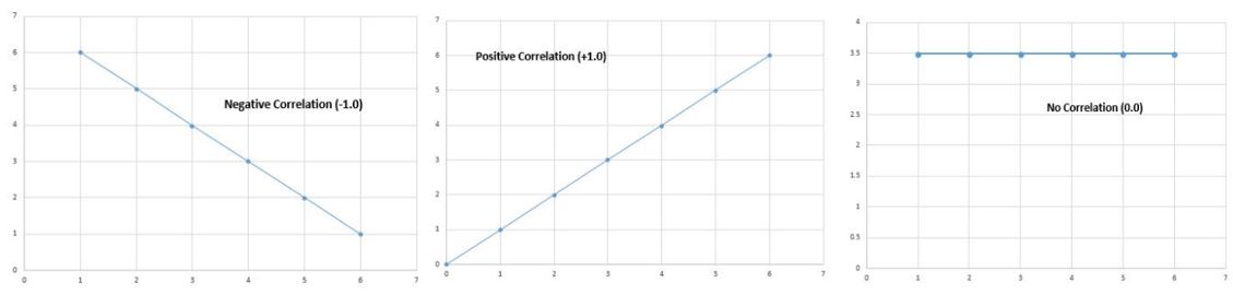
• As much as the correlation coefficient is closer to +1 or -1, it indicates positive (+1) or negative (-1) correlation between the arrays. Positive correlation means that if the values in one array are increasing, the values in the other array increase as well. A correlation coefficient that is closer to 0, indicates no or weak correlation.

• The equation for the correlation coefficient is:

  

  where 

  

  are the sample means AVERAGE(array1) and AVERAGE(array2).

Example

The following example returns the correlation coefficient of the two data sets in columns A and B.

Need more help?

You can always ask an expert in the Excel Tech Community or get support in the Answers community.

What is the Correlation Coefficient?

The correlation coefficient of a data set is a statistical number that tells how strongly two variables are related to each other. It can be said that it is the percentage of the relation between two variables (x and y). It can’t be greater than 100% and less than -100%.

The correlation coefficient falls between -1.0 and +1.0.

A negative correlation coefficient tells us that if one variable increases, other variable decreases. A correlation of -1.0 is a perfect negative correlation. This means that if x increases by 1 unit, y decreases by 1 unit.

A positive correlation coefficient tells us that if one variable’s value increases, other variable’s value also increases. This means that if x increases by 1 unit, y also increases by 1 unit.

The correlation of 0 says that there is no relation between two variables what so ever.

The Mathematical formula of Correlation Coefficient is:

=Coveriance_xy/(Std_x*Std_y)

Coveriance_xy is the covariance (sample or population) of data set.

Std_x= It is Standard Deviation (sample or population) of Xs.

Std_y= It is Standard Deviation (sample or population) of Ys.

How to Calculate the Correlation Coefficient in Excel?

If you need to calculate the correlation in excel, you do not need to use the mathematical formula.  You can use these methods

1. Calculating Correlation Coefficient using COREL function.
2. Calculating Correlation Coefficient using Analysis Toolpak.

Let’s see an example to know how to calculate the correlation coefficient in excel.

Example of Calculation of correlation coefficient in excel

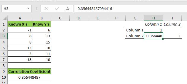
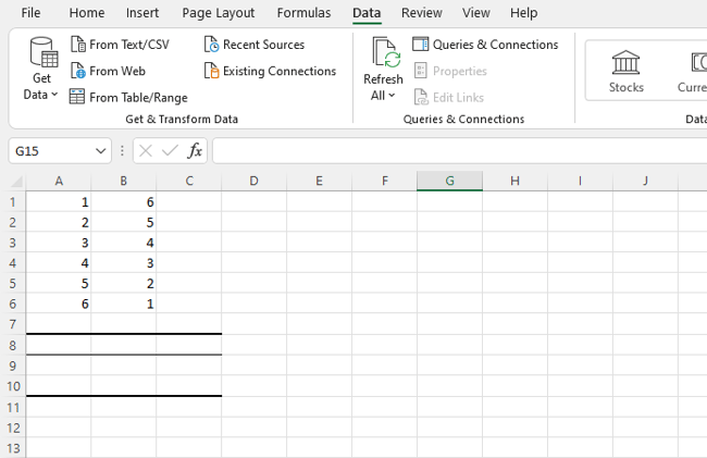
Here I have a sample data set. We have xs in range A2:A7 and ys in B2:B7.

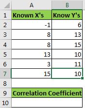
We need to calculate the correlation coefficient of xs and ys.

Using Excel CORREL Function

Syntax of the CORREL function:

array1: This is the first set of values (xs)

array2: It is the second set of values (ys).

Note: the array 1 and array 2 should be of the same size.

Let’s use the CORREL function to get the correlation coefficient. Write this formula in A10.

We get a correlation of 0.356448487 or 36% between x and y.

Using Excel Analysis Toolpak

To calculate correlation using analysis toolpak follow these steps:

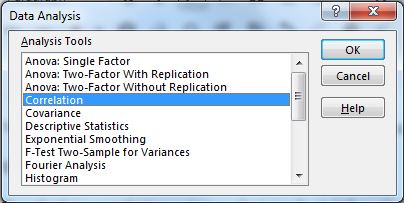
• Go to the Data tab on the ribbon. To the left most corner, you will find the data analysis option. Click on it. If you can’t see it, you first need to install the analysis toolpak.

• From the available options, select Correlation.

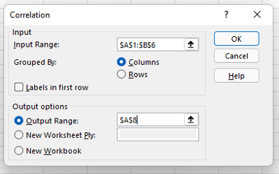
• Select the input range as A2:B7. Select the output range where you want to see your output.

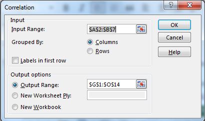
• Hit OK button. You have your correlation coefficient in the desired range. It is the exact same value as returned by the CORREL function.

How correlation is being calculated?

To understand how we are getting this value, we need to find it manually. This will clear our doubts.

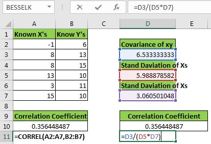
As we know the correlation coefficient is:

=Coveriance_xy/(Std_x*Std_y)

First, we need to calculate the covariance. We can use the COVERIACE.S function of excel to calculate it.

=COVARIANCE.S(A2:A7,B2:B7)

Next, let’s calculate the standard deviation of x and y using the STDEV.S function.

Now in cell D10, write this formula.

This is equivalent to =Covariance_xy/(Std_x*Std_y). You can see that we get the exact same value as given by the CORREL function. Now you know how we have derived the correlation coefficient in excel.

Note: In the above example, we have used COVARIANCE.S (covariance of the sample) and STDEV.S (standard deviation of the sample). The correlation coefficient will be the same if you use COVARIANCE.P and STDEV.P.  As long as they both are of the same category there will be no difference. If you use COVARIANCE.S (covariance of the sample) and STDEV.P (standard deviation of the population) then the result will be different and incorrect.

So yeah guys, this is how we can calculate correlation coefficient in excel. I hope this was explanatory enough to explain the correlation coefficient. You can now create your own correlation coefficient calculator in excel.

Related Articles:

Calculate INTERCEPT in Excel

Calculating SLOPE in Excel

Regressions in Excel

How to Create Standard Deviation Graph

Descriptive Statistics in Microsoft Excel 2016

How to Use Excel NORMDIST Function

Pareto Chart and Analysis

Popular Articles:

50 Excel Shortcut to Increase Your Productivity

The VLOOKUP Function in Excel

COUNTIF in Excel 2016

How to Use SUMIF Function in Excel

The correlation coefficient (a value between -1 and +1) tells you how strongly two variables are related to each other. We can use the CORREL function or the Analysis Toolpak add-in in Excel to find the correlation coefficient between two variables.

— A correlation coefficient of +1 indicates a perfect positive correlation. As variable X increases, variable Y increases. As variable X decreases, variable Y decreases.

— A correlation coefficient of -1 indicates a perfect negative correlation. As variable X increases, variable Z decreases. As variable X decreases, variable Z increases.

— A correlation coefficient near 0 indicates no correlation.

To use the Analysis Toolpak add-in in Excel to quickly generate correlation coefficients between multiple variables, execute the following steps.

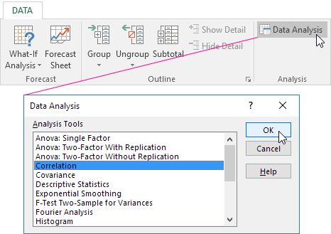
1. On the Data tab, in the Analysis group, click Data Analysis.

Note: can’t find the Data Analysis button? Click here to load the Analysis ToolPak add-in.

2. Select Correlation and click OK.

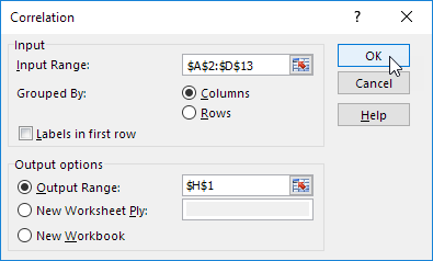
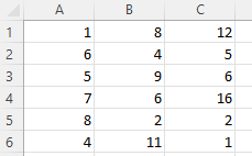
3. For example, select the range A1:C6 as the Input Range.

4. Check Labels in first row.

5. Select cell A8 as the Output Range.

6. Click OK.

Result.

Conclusion: variables A and C are positively correlated (0.91). Variables A and B are not correlated (0.19). Variables B and C are also not correlated (0.11)
. You can verify these conclusions by looking at the graph.

The correlation coefficient reflects to the degree of interrelation between the two indicators. It always takes the value from -1 to 1. If the coefficient is located about 0, then there is no connection between the variables.

If the value is close to one (from 0. 9, for example), then between the observed objects there is the strong direct relationship. If the coefficient is close to the other extreme point of the range (-1), then between the variables there is a strong inverse relationship. When the value is somewhere in the middle from 0 to 1 or from 0 to -1, then it is a weak connection (direct or reverse). This relationship is usually not taken into account: it is believed that it is not.



The calculation of the correlation coefficient in Excel

Let`s consider the example to the methods of calculating the correlation coefficient, the particular qualitie of the direct and inverse relationship between the variables.

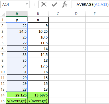
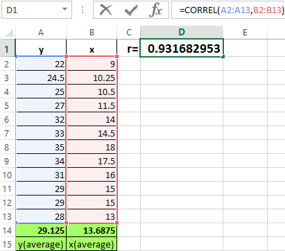
There are the values of x and y:

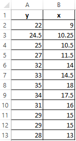
Y is an independent variable, x is an independent variable. It is necessary to find the strength (strong / weak) and the direction (direct / inverse) of the connection between them. The formula of the correlation coefficient looks like that:

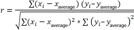
To make it easier to understand, we will break it into several simple elements.

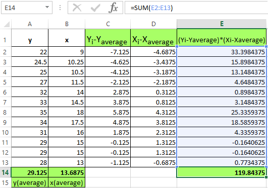
1. Find the mean values of the variables using the AVERAGE function:



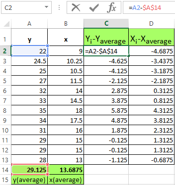
2. Calculate the difference between each y and y mean, each x and x medium. We use to the mathematical operator «-».



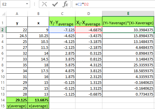
3. You need multiply now the differences found:



4. Find the sum of the values in this column. This will be the numerator.



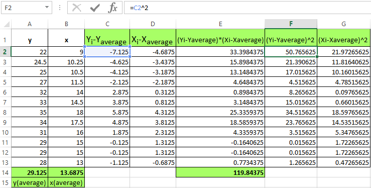
5. To calculate the difference denominator of y and y-average, x and x-average. It is necessary to erect it a square.



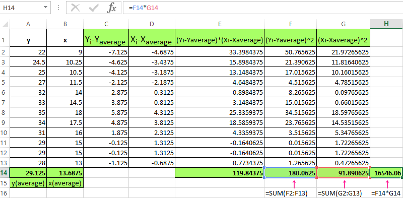
6. Find the sum of the values in the received columns (using the AUTO-SUM function) and multiply these values.



7. The result is squared (SQRT function).



8. It remains to calculate the quotient (the numerator and denominator are already known).

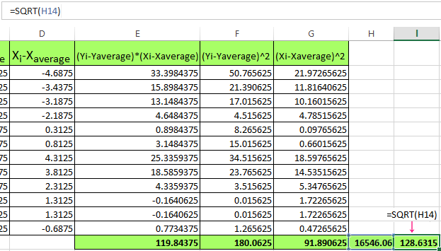
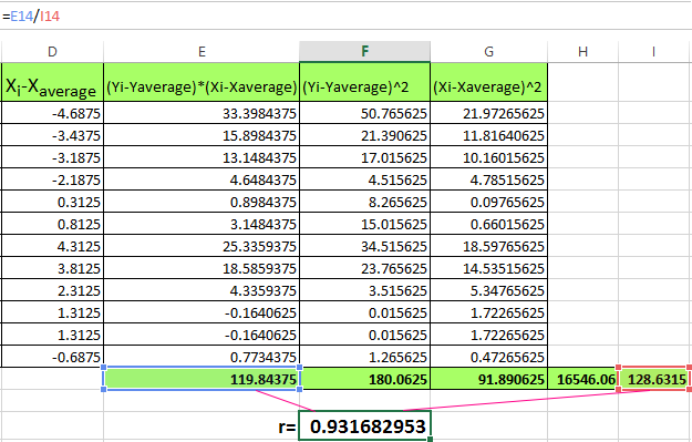
The strong direct link is defined between the variables.

The built-in CORREL function allows you to avoid of complex calculations. We calculate the coefficient of pair correlation in Excel with its help. You need to call the function wizard and to find the right one. The arguments of the function are an array of values of y and an array of values of x:

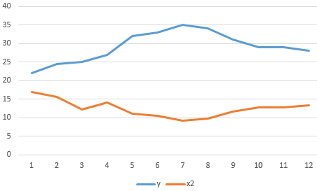
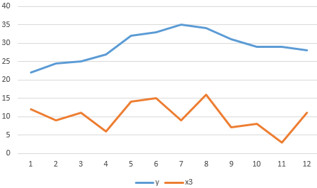
We show the values of the variables on the chart:

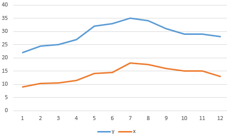
There is a strong interconnection between y and x, because the lines run almost parallel to each other. The interconnection is straight: grows y — grows x, decreases y — decreases x.



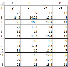
The matrix of paired correlation coefficients in Excel

The correlation matrix is the table, at the intersection of rows and columns of which are the correlation coefficients between the corresponding values. It makes sense to build it for several variables.

The matrix of correlation coefficients in Excel is constructed using the «Correlation» tool from the «Data analysis» package.

1. On the «Data» tab in the «Analysis» group, we need to open the «Data analysis» package (for the 2007 version). If the button is not available, you need to add it («Excel Options»- «Add-ins»). In the analysis tools list, zou need to select «Correlation».



2. Click OK and set the parameters for data analysis. The input interval is the range of cells with values. The grouping — by columns (analyzed data are grouped into columns). The output interval is the reference to the cell from which the matrix is to be built. The size of the range will be determined automatically.



3. After pressing OK, the correlation matrix appears in the output range. At the intersection of rows and columns there are the correlation coefficients. If the coordinates are the same, the value 1 is output.

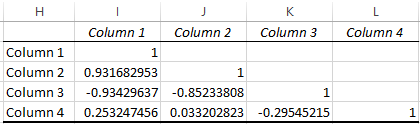
Between the values of y and x1 is found the strong direct connection. There is a strong feedback between x1 and x2. There is practically no connection with the values in the column x3.

Let`s show graphically the correlation relations using graphs.

1. The strong direct connection between y and x.



2. The strong feedback between y and x2. The values change occur parallel to each other, but if y grows, x falls. The values of y increase — the values of x decrease.



3. The absence of the relationship between the values of y and x3. The changes in x3 occur chaotically and its do not correlate with changes in y.

Download calculation coefficient of pair correlation in Excel

Why do we need such the coefficient? It`s need for determining of interconnection between the observed phenomena and forecasting.

Microsoft Excel lets you do more than simply create spreadsheets — you can also use the software to calculate key functions, such as the relationship between two variables. Known as the correlation coefficient, this metric is useful for measuring the impact of one operation on another to inform business operations.

Not confident in your Excel skills? No problem. Here’s how to calculate — and understand — the correlation coefficient in Excel.

A correlation coefficient of +1 indicates a “perfect positive correlation”, which means that as variable X increases, variable Y increases at the same rate. A correlation value of -1, meanwhile, is a “perfect negative correlation”, which means that as variable X increases, variable Y decreases at the same rate. Correlation analysis may also return results anywhere between -1 and +1, which indicates that variables change at similar but not identical rates.

Correlation values can help businesses evaluate the impact of specific actions on other actions. For example, companies may find that as spending on social media marketing increases, so does customer engagement, indicating that more spending might make sense.

Or they may find that specific advertising campaigns result in a correlated decrease of customer engagement, in turn suggesting the need for a reevaluation of current efforts. The discovery that variables do not correlate can also be valuable; while common sense might suggest that a new function or feature in your product would correlate with increased engagement, it might have no measurable impact. Correlation analysis allows companies to view this relationship (or lack thereof) and make sound strategic decisions.

So how do you calculate the correction coefficient in Excel? Simple! Follow these steps:

1. Open Excel.

Step one: Open Excel and start a new worksheet for your correlated variable data. Enter the data points of your first variable in column A and your second variable in column B. You can add additional variables as well in columns C, D, E, etc. — Excel will provide a correlation coefficient for each one.

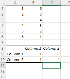
In the example below, we’ve entered six rows of data in column A and six in column B.

2. Install the Analysis Toolpak.

Next up? If you don’t have it, install the Excel Analysis Toolpak.

Select “File”, then “Options,” and you’ll see this screen:

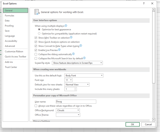
Select “Add-Ins” and then click on “Go”.

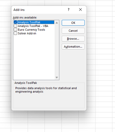
Now, check the box that says “Analysis ToolPak” and click “Ok”.

3. Select “Data” from the top bar menu.

Once you have the ToolPak installed, select “Data” from the top Excel bar menu. This provides you with a submenu that contains a variety of analysis options for your data.

4. Select “Data Analysis” in the top right-hand corner.

Now, look for “Data Analysis” in the top right-hand corner and click on it to get this screen:

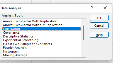
5. Select Correlation.

Select Correlation from the menu and click “OK.”

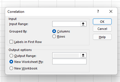
6. Define your data range and output.

Now define your data range and output. You can simply left-click and drag your cursor across the data you want to select, and it will auto-populate in the Correlation box. Finally, select an output range for your correlation data — we’ve chosen A8. Then, click “Ok”.

7. Evaluate your correlation coefficient.

Your correlation results will now be displayed. In our example, values in column 1 and column 2 have a perfect negative correlation; as one goes up, the other goes down at the same rate.

The Excel Correlation Matrix

Excel correlation results are also known as an Excel correlation matrix. In the example above, our two columns of data produced a perfect correction matrix of 1 and -1. But what happens if we produce a correlation matrix with a less ideal data set?

Here’s our data:

And here’s the matrix:

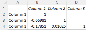
Cell C4 in the matrix gives us the correlation between Column 3 and Column 2, which is a very weak 0.01025, while Column 1 and Column 3 yield a stronger negative correlation of -0.17851. By far the strongest correlation, however, is between Column 1 and Column 2 at -0.66891.

So what does this mean in practice? Let’s say we were examining the impact of specific actions on the efficacy of a social media campaign, where Column 1 represents the number of visitors who click through on social advertisements and Columns 2 and 3 represent two different marketing taglines. The correlation matrix shows a strong negative correlation between Columns 1 and 2, which suggests that the Column 2 version of the tagline significantly decreased overall user engagement, while Column 3 drove only a slight decrease.

Regularly creating Excel matrices can help companies better understand the impact of one variable on another and determine what (if any) negative or positive effects may exist.

The Excel Correlation Formula

If you prefer to enter the correlation formula yourself, that’s also an option. Here’s what it looks like:

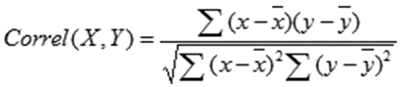
X and Y are your measurements, ∑ is the sum, and the X and Y with the bars over them indicate the mean value of the measurements. You would calculate it as follows:

• Calculate the sum of variable X minus the mean of X.
• Calculate the sum of variable Y minus the mean of Y.
• Multiply those two results and set that number aside (this is the first result).
• Square the sum of X minus the mean of X. Square the sum of Y minus the mean of Y. Multiply those two numbers.
• Take the square root (this is the second result).
• Divide the first result by the second result.
• You get the correlation coefficient.

Easy, right? Yes and no. While plugging in the numbers isn’t complicated, it’s often more trouble than it’s worth to create and manage this formula. The built-in Excel Toolpak is often a simpler (and faster) way to pinpoint coefficients and discover key relationships.

Correlation ≠ Not Causation

No article about correlation is complete without a mention that it does not equal causation. In other words, just because two variables rise or fall together doesn’t mean that one variable is the cause of the other variable’s increase or decrease.

Consider a few very strange examples.

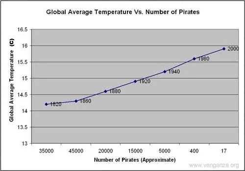
This image shows a near-perfect negative correlation between the number of pirates and the global average temperature — as pirates became more scarce, the average temperature increased.

The problem? While these two variables are correlated, there’s no causal link between the two; higher temperatures did not reduce the pirate population and fewer pirates did not cause global warming.

While correlation is a powerful tool, it only indicates the direction of increase or decrease between two variables — not the cause of this increase or decrease. To discover causal links, companies must increase or decrease one variable and observe the impact. For example, if correlation shows that customer engagement goes up with social media spending, it’s worth opting for a slight increase in spending followed by a measurement of results. If more spending leads directly to increased engagement, the link is both correlated and causal. If not, there may be one (or more) factors that underpin the increase of both variables.

Keeping Up with the Correlations

Excel correlations offer a solid starting point for marketing, sales, and spending strategy development, but they don’t tell the whole story. As a result, it’s worth using Excel’s built-in data analysis options to quickly evaluate the correlation between two variables and use this data as a jumping-off point for more in-depth analysis.

Excel is a powerful tool that has some amazing functions and functionalities when working with statistics.

Finding a correlation between two data series is one of the most common statistical calculation when working with large datasets,

I was working as a financial analyst a few years ago, and although we were not heavily involved in statistical data, finding correlation was something we still had to do quite often.

In this tutorial, I will show you two really easy ways to calculate correlation coefficient in Excel. There is already a built-in function to do this, and you can also use the Data Analysis Toolpak.

So let’s get started!

What is the Correlation Coefficient?

Since this is not a statistics class, let me briefly explain what is the correlation coefficient, and then we’ll move on to the section where we calculate the correlation coefficient in Excel.

A correlation coefficient is a value that tells you how closely two data series are related.

A commonly used example is the weight and height of 10 people in a group. If we calculate the correlation coefficient for the height and weight data for these people, we will get a value between -1 and 1.

A value less than zero indicates a negative correlation, which means that if the height increases then the weight decreases, or if the weight increases at then the height decrease.

And a value more than zero indicates a positive correlation, which means that if the height increases then the weight increases, and if the height decreases then the weight decreases.

The closer the value is to 1, the stronger is the positive correlation. So a value of .8 would indicate that the height and weight data are strongly correlated.

Note: There are different types of correlation coefficients and statistics, but in this tutorial, we’ll be looking at the most common one which is the Pearson correlation coefficient

Now, let’s see how to calculate this correlation coefficient in Excel.

Calculating Correlation Coefficient in Excel

As I mentioned, there are a couple of ways you can calculate the correlation coefficient in Excel.

Using CORREL Formula

CORREL is a statistics function that was introduced in Excel 2007.

Suppose you have a data set as shown below where you want to calculate the correlation coefficient between the height and the weight of 10 people.

Below is the formula that would do this:

=CORREL(B2:B12,C2:C12)

The above CORREL function takes two arguments – the series with the height data points and the series with the weight data points.

And that’s it!

As soon as you hit enter, Excel does all the calculations in the back-end it gives you one single Pearson correlation coefficient number.

In our example, that value is a little over .5, which indicates that there is a fairly strong positive correlation.

This method is best used if you have two series and all you want is the correlation coefficient.

But if you have multiple series and you want to find out the correlation coefficient of all these series, then you can also consider using the data analysis tool pack in Excel (covered next)

Using the Data Analysis Toolpak

Excel has a Data Analysis Toolpak that can be used to quickly calculate various statistics values (including getting the correlation coefficient).

But the Data Analysis Toolpak is disabled by default in Excel. So the first step would be to enable the data analysis tool back and then use that to calculate the Pearson correlation coefficient in Excel.

Enabling the Data Analysis Toolpak

Below are the steps to enable the Data Analysis Toolpak in Excel:

1. Click the File tab
2. Click on Options
3. In the Excel Options dialog box that opens up, click on the Add-ins option in the sidebar pane
4. In the Manage drop-down, select Excel add-ins
5. Click on Go. This will open the add-ins dialog box
6. Check the Analysis Toolpak option
7. Click on Ok

The above steps would add a new group in the Data tab in the Excel ribbon called Analysis. Within this group, you would have the Data Analysis option

Calculating the Correlation Coefficient Using Data Analysis Toolpak

Now that you have the analysis tool back available in the ribbon, let’s see how to calculate the correlation coefficient using it.

Suppose you have a data set as shown below and you want to find out the correlation between the three series (height and weight, height and income, and weight and income)

Below are the steps to do this:

1. Click the Data tab
2. In the Analysis group, click on the Data Analysis option
3. In the Data Analysis dialog box that opens up, click on ‘Correlation’
4. Click OK. This will open the Correlation dialog box
5. For input range, select the three series – including the headers
6. For ‘Grouped by’, make sure ‘Columns’ is selected
7. Select the option – ‘Label in First Row’. This will make sure that in the resulting data would have the same headers and it would be a lot easier to understand the results
8. In the Output options, choose where you want the resulting table. I’m going to go with cell G1 on the same worksheet. You can also choose to get your results in a new worksheet or a new workbook
9. Click OK

As soon as you do this, Excel would calculate the correlation coefficient for all the series and give you a table as shown below:

Note that the resulting table is static, and would not update in case any of the data points in your table change. In case of any change, you will have to repeat the above steps again to generate a new table of correlation coefficients.

So these are two quick and easy methods to calculate correlation coefficient in Excel.

I hope you found this tutorial useful!

Other Excel tutorials you may also like:

• How to Calculate Standard Deviation In Excel (Step-by-Step)
• How to Find Outliers in Excel (and how to handle these)
• Calculating Moving Average in Excel [Simple, Weighted, & Exponential]
• How to Calculate Compound Annual Growth Rate (CAGR) in Excel
• One Variable Data Table in Excel
• Two Variable Data Table in Excel
• Scenario Manager in Excel
• Using Solver in Excel
• How to Get Descriptive Statistics in Excel?
• Calculate the Coefficient of Variation (CV) in Excel

In this guide, I will show you how to perform a Pearson correlation test in Microsoft Excel. This includes determining the Pearson correlation coefficient as well as a p value for the statistical test.

I have discussed how to perform a Spearman’s rank correlation test in Excel previously.

A Pearson correlation is a statistical test to determine the association between two continuous variables.

The output is given as the Pearson correlation coefficient (r) which is a value ranging from -1 to 1 to indicate the strength of the association.

The following values of r indicate the direction and strength of the association.

• r = -1: A perfect negative association
• r = 0: No association
• r = +1: A perfect positive association

If you want to learn more about about the test, including the test assumptions, then check out my Pearson correlation explained article.

How to perform a Pearson correlation test in Excel

In Excel, there is a function available to calculate the Pearson correlation coefficient. However, there is no simple means of calculating a p-value for this. A way around this is to firstly calculate a t statistic which will then be used to determine the p-value.

1. Calculate the Pearson correlation coefficient in Excel

In this section, I will show you how to calculate the Pearson correlation coefficient in Excel, which is straightforward.

In Excel, click on an empty cell where you want the correlation coefficient to be entered. Then enter the following formula.

=PEARSON(array1, array2)

Simply replace ‘array1‘ with the range of cells containing the first variable and replace ‘array2‘ with the range of cells containing the second variable.

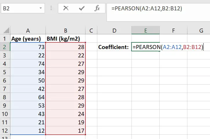
For the example above, the Pearson correlation coefficient (r) is ‘0.76‘.

2. Calculate the t-statistic from the coefficient value

The next step is to convert the Pearson correlation coefficient value to a t-statistic. To do this, two components are required: r and the number of pairs in the test (n).

In order to determine the number of pairs, simply count them manually or use the count function (=COUNT). Each pair should be a pair, so remove any entries that are not a pair.

The equation used to convert r to the t-statistic can be found below.

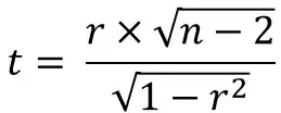
The formula to do this in Excel can be found below.

=(r*SQRT(n-2))/(SQRT(1-r^2))

Simply replace the ‘r‘ with the correlation coefficient value and replace the ‘n‘ with the number of observations in the analysis.

For the example in this guide, the formula used in Excel can be seen below.

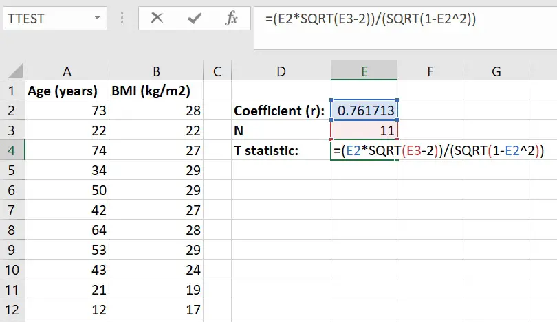
Note, if your coefficient value is negative, then use the following formula:

=(ABS(r)*SQRT(n-2))/(SQRT(1-ABS(r)^2))

The addition of the ABS function converts the coefficient value to an absolute (positive) number. Otherwise, a negative coefficient value will bring up an error.

3. Calculate the p-value from the t statistic

The final step in the process of calculating the p-value for a Pearson correlation test in Excel is to convert the t-statistic to a p-value.

Before this can be done, we just need to calculate a final piece of information: the number of degrees of freedom (DF). The DF can be found by subtracting 2 from n (n – 2).

Now we are ready to calculate the p-value. To do this, simply use the =TDIST function in Excel.

Simply enter the formula below.

=TDIST(x, deg_freedom, tails)

Replace the ‘x‘ with the t statistic created previously and replace the ‘deg_freedom‘ with the DF. Finally, for the tails, enter the number ‘1‘ for a one-tailed analysis or a ‘2‘ for a two-tailed analysis. If you are unsure about which to use, use a two-tailed analysis (‘2‘).

Below is a screenshot for how this looks in Excel by using the example.

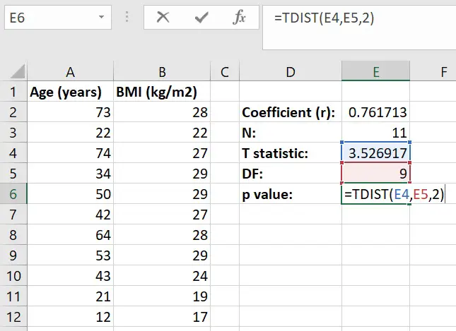
In the example, the p value is ‘0.006‘. Therefore, there is a significant positive correlation (r=0.76) between participant ages and their BMI.

Conclusion

There is no easy way to calculate a p value for a Pearson correlation test in Excel. However, by calculating the Pearson correlation coefficient this can be converted to a t-statistic, which in turn can be used to calculate a p-value.

Microsoft Excel version used: 365 ProPlus

If you’ve ever learnt some statistics, then you’ve probably come across the correlation coefficient.

But can you calculate this in Excel?

Yes, you can!

Excel can be a great tool for a statistician when you know how to use it.

In this post, I’ll show you 3 ways to calculate the correlation coefficient in Excel.

Video Tutorial

What is a Correlation Coeffecient?

The correlation coefficient is also known as the Pearson Correlation Coefficient and it is a measurement of how related two variables are.

The calculation can have a value between 0 and 1.

A value of 0 indicates the two variables are highly unrelated and a value of 1 indicates they are highly related.

For example, you might have data on height (meters) and weight (kilograms) for a sample of people and want to know if these two variables are related.

Intuitively, you would think a person’s height and weight are related, but the correlation coefficient will show you mathematically how related or unrelated these are.

Correlation Coefficient Formula

The correlation coefficient r can be calculated with the above formula where x and y are the variables which you want to test for correlation.

In this example, the x variable is the height and the y variable is the weight. r is then the correlation between height and weight.

Calculating the Correlation Coefficient from the Definition

Let’s see how we can calculate this in Excel based on the above definition.

There are quite a few steps involved to calculate the correlation coefficient from scratch.

1. Calculate the average height.

   = AVERAGE ( C3:C12 )

2. Calculate the average weight.

   = AVERAGE ( D3:D12 )

3. Calculate the difference between the height and average height for each data point. This formula will need to be copied down for each row.

   = C3 - $C$14

4. Calculate the difference between the weight and average weight for each data point. This formula will need to be copied down for each row.

   = D3 - $D$14

5. Calculate the square of the difference from step 3 for each row.

   = POWER ( F3, 2 )

6. Calculate the square of the difference from step 4 for each row.

   = POWER ( G3, 2 )

7. Calculate the product of differences from step 3 and 4 for each row.

   = F3 * G3

8. Calculate the sum of the squared differences from step 5.

   = SUM ( H3:H12 )

9. Calculate the sum of the squared differences from step 6.

   = SUM ( I3:I12 )

10. Calculate the sum of the product of differences from step 7.

    = SUM ( J3:J12 )

11. Calculate the correlation with the following formula.

    = J14 / ( SQRT ( H14 ) * SQRT ( I14 ) )

It’s quite an involved calculation with a lot of intermediate steps.

Thankfully Excel has a built in function for getting the correlation which makes the calculation much more simple.

CORREL Function

This is a function specifically for calculating the Pearson correlation coefficient in Excel.

It’s very easy to use. It takes two ranges of values as the only two arguments.

= CORREL ( Variable1, Variable2 )

• Variable1 and Variable2 are the two variables which you want to calculate the Pearson Correlation Coefficient between.
• These are required inputs and must be a single column or single row array of numbers. Variable1 and Variable2 must also have the same dimension.

= CORREL ( Height, Weight )

The above formula is what you would need to calculate the correlation between height and weight.

Wow, so much easier than calculating it from scratch!

This method is also dynamic. If your data changes, the correlation calculation will update to reflect the new data.

Statistical Tools

Excel comes with a powerful statistical tools add-in, but you need to enable it to use it first and it’s quite hidden.

To enable the Analysis ToolPak:

1. Go to the File tab and then choose Options.
2. Go to the Add-ins tab in the Excel Options.
3. Choose Excel Add-ins from the drop-down list and press the Go button.
4. Check the Analysis ToolPak option from the available add-ins.
5. Press the OK button.

You will now have a Data Analysis command available in the Data tab and you can click on this to open up the Analysis ToolPak.

This will open up the Data Analysis menu and you can then select Correlation from the options and press the OK button.

This will open up the Data Analysis Correlation menu.

1. Supply the Input Range for the correlation calculation. This should be a range with numerical values organized into columns or rows.
2. Select the Group By option of Columns or Rows. This example has the data organized by columns as values for height are all in one column and values for weight are in a separate column.
3. Select whether or not your input range has Labels in the first row. These labels are used later in the output so it’s best to select an input range that includes the labels.
4. Select where to place the output in the Output options. You can choose from a location in the current sheet, a location in a new sheet, or a new workbook.
5. Press the OK button create the calculation.

This will output a correlation matrix.

This means if you have more than two columns of variable, the matrix will contain the correlation coefficient for all combinations of variables.

The drawback of this method is the output is static. If your data changes, you will need to rerun the data analysis to update the correlation matrix.

Conclusions

Correlation is a very useful statistic to determine if your data is related.

The mathematical formula can be intimidating though, especially when trying to calculate it in Excel.

Thankfully there are a few easy ways to implement this calculation in Excel.