Copying rows in excel - Word и Excel - помощь в работе с программами

When you move or copy rows and columns, by default Excel moves or copies all data that they contain, including formulas and their resulting values, comments, cell formats, and hidden cells.

When you copy cells that contain a formula, the relative cell references are not adjusted. Therefore, the contents of cells and of any cells that point to them might display the #REF! error value. If that happens, you can adjust the references manually. For more information, see Detect errors in formulas.

You can use the Cut command or Copy command to move or copy selected cells, rows, and columns, but you can also move or copy them by using the mouse.

By default, Excel displays the Paste Options button. If you need to redisplay it, go to Advanced in Excel Options. For more information, see Advanced options.

Select the cell, row, or column that you want to move or copy.
Do one of the following:
- To move rows or columns, on the Home tab, in the Clipboard group, click Cut or press CTRL+X.
- To copy rows or columns, on the Home tab, in the Clipboard group, click Copy or press CTRL+C.
Right-click a row or column below or to the right of where you want to move or copy your selection, and then do one of the following:
- When you are moving rows or columns, click Insert Cut Cells.
- When you are copying rows or columns, click Insert Copied Cells.
Tip: To move or copy a selection to a different worksheet or workbook, click another worksheet tab or switch to another workbook, and then select the upper-left cell of the paste area.

Note: Excel displays an animated moving border around cells that were cut or copied. To cancel a moving border, press Esc.

By default, drag-and-drop editing is turned on so that you can use the mouse to move and copy cells.

Select the row or column that you want to move or copy.
Do one of the following:
- Cut and replace
  Point to the border of the selection. When the pointer becomes a move pointer , drag the rows or columns to another location. Excel warns you if you are going to replace a column. Press Cancel to avoid replacing.
- Copy and replace Hold down CTRL while you point to the border of the selection. When the pointer becomes a copy pointer , drag the rows or columns to another location. Excel doesn’t warn you if you are going to replace a column. Press CTRL+Z if you don’t want to replace a row or column.
- Cut and insert Hold down SHIFT while you point to the border of the selection. When the pointer becomes a move pointer , drag the rows or columns to another location.
- Copy and insert Hold down SHIFT and CTRL while you point to the border of the selection. When the pointer becomes a move pointer , drag the rows or columns to another location.
Note: Make sure that you hold down CTRL or SHIFT during the drag-and-drop operation. If you release CTRL or SHIFT before you release the mouse button, you will move the rows or columns instead of copying them.

Note: You cannot move or copy nonadjacent rows and columns by using the mouse.

If some cells, rows, or columns on the worksheet are not displayed, you have the option of copying all cells or only the visible cells. For example, you can choose to copy only the displayed summary data on an outlined worksheet.

Select the row or column that you want to move or copy.
On the Home tab, in the Editing group, click Find & Select, and then click Go To Special.
Under Select, click Visible cells only, and then click OK.
On the Home tab, in the Clipboard group, click Copy or press Ctrl+C. .
Select the upper-left cell of the paste area.

Tip: To move or copy a selection to a different worksheet or workbook, click another worksheet tab or switch to another workbook, and then select the upper-left cell of the paste area.
On the Home tab, in the Clipboard group, click Paste or press Ctrl+V.

If you click the arrow below Paste , you can choose from several paste options to apply to your selection.

Excel pastes the copied data into consecutive rows or columns. If the paste area contains hidden rows or columns, you might have to unhide the paste area to see all of the copied cells.

When you copy or paste hidden or filtered data to another application or another instance of Excel, only visible cells are copied.

Select the row or column that you want to move or copy.
On the Home tab, in the Clipboard group, click Copy or press Ctrl+C.
Select the upper-left cell of the paste area.
On the Home tab, in the Clipboard group, click the arrow below Paste , and then click Paste Special.
Select the Skip blanks check box.

Double-click the cell that contains the data that you want to move or copy. You can also edit and select cell data in the formula bar.
Select the row or column that you want to move or copy.
On the Home tab, in the Clipboard group, do one of the following:
- To move the selection, click Cut or press Ctrl+X.
- To copy the selection, click Copy or press Ctrl+C.
In the cell, click where you want to paste the characters, or double-click another cell to move or copy the data.
On the Home tab, in the Clipboard group, click Paste or press Ctrl+V.
Press ENTER.

Note: When you double-click a cell or press F2 to edit the active cell, the arrow keys work only within that cell. To use the arrow keys to move to another cell, first press Enter to complete your editing changes to the active cell.

When you paste copied data, you can do any of the following:

Paste only the cell formatting, such as font color or fill color (and not the contents of the cells).
Convert any formulas in the cell to the calculated values without overwriting the existing formatting.
Paste only the formulas (and not the calculated values).

Procedure

Select the row or column that you want to move or copy.
On the Home tab, in the Clipboard group, click Copy or press Ctrl+C.
Select the upper-left cell of the paste area or the cell where you want to paste the value, cell format, or formula.
On the Home tab, in the Clipboard group, click the arrow below Paste , and then do one of the following:
- To paste values only, click Values.
- To paste cell formats only, click Formatting.
- To paste formulas only, click Formulas.

When you paste copied data, the pasted data uses the column width settings of the target cells. To correct the column widths so that they match the source cells, follow these steps.

Select the row or column that you want to move or copy.
On the Home tab, in the Clipboard group, do one of the following:
- To move cells, click Cut or press Ctrl+X.
- To copy cells, click Copy or press Ctrl+C.
Select the upper-left cell of the paste area.

Tip: To move or copy a selection to a different worksheet or workbook, click another worksheet tab or switch to another workbook, and then select the upper-left cell of the paste area.
On the Home tab, in the Clipboard group, click the arrow under Paste , and then click Keep Source Column Widths.

You can use the Cut command or Copy command to move or copy selected cells, rows, and columns, but you can also move or copy them by using the mouse.

Select the cell, row, or column that you want to move or copy.
Do one of the following:
- To move rows or columns, on the Home tab, in the Clipboard group, click Cut or press CTRL+X.
- To copy rows or columns, on the Home tab, in the Clipboard group, click Copy or press CTRL+C.
Right-click a row or column below or to the right of where you want to move or copy your selection, and then do one of the following:
- When you are moving rows or columns, click Insert Cut Cells.
- When you are copying rows or columns, click Insert Copied Cells.
Tip: To move or copy a selection to a different worksheet or workbook, click another worksheet tab or switch to another workbook, and then select the upper-left cell of the paste area.

Note: Excel displays an animated moving border around cells that were cut or copied. To cancel a moving border, press Esc.

Select the row or column that you want to move or copy.
Do one of the following:
- Cut and insert
  Point to the border of the selection. When the pointer becomes a hand pointer , drag the row or column to another location
- Cut and replace Hold down SHIFT while you point to the border of the selection. When the pointer becomes a move pointer , drag the row or column to another location. Excel warns you if you are going to replace a row or column. Press Cancel to avoid replacing.
- Copy and insert Hold down CTRL while you point to the border of the selection. When the pointer becomes a move pointer , drag the row or column to another location.
- Copy and replace Hold down SHIFT and CTRL while you point to the border of the selection. When the pointer becomes a move pointer , drag the row or column to another location. Excel warns you if you are going to replace a row or column. Press Cancel to avoid replacing.
Note: Make sure that you hold down CTRL or SHIFT during the drag-and-drop operation. If you release CTRL or SHIFT before you release the mouse button, you will move the rows or columns instead of copying them.

Note: You cannot move or copy nonadjacent rows and columns by using the mouse.

Double-click the cell that contains the data that you want to move or copy. You can also edit and select cell data in the formula bar.
Select the row or column that you want to move or copy.
On the Home tab, in the Clipboard group, do one of the following:
- To move the selection, click Cut or press Ctrl+X.
- To copy the selection, click Copy or press Ctrl+C.
In the cell, click where you want to paste the characters, or double-click another cell to move or copy the data.
On the Home tab, in the Clipboard group, click Paste or press Ctrl+V.
Press ENTER.

Note: When you double-click a cell or press F2 to edit the active cell, the arrow keys work only within that cell. To use the arrow keys to move to another cell, first press Enter to complete your editing changes to the active cell.

When you paste copied data, you can do any of the following:

Paste only the cell formatting, such as font color or fill color (and not the contents of the cells).
Convert any formulas in the cell to the calculated values without overwriting the existing formatting.
Paste only the formulas (and not the calculated values).

Procedure

Select the row or column that you want to move or copy.
On the Home tab, in the Clipboard group, click Copy or press Ctrl+C.
Select the upper-left cell of the paste area or the cell where you want to paste the value, cell format, or formula.
On the Home tab, in the Clipboard group, click the arrow below Paste , and then do one of the following:
- To paste values only, click Paste Values.
- To paste cell formats only, click Paste Formatting.
- To paste formulas only, click Paste Formulas.

You can move or copy selected cells, rows, and columns by using the mouse and Transpose.

Select the cells or range of cells that you want to move or copy.
Point to the border of the cell or range that you selected.
When the pointer becomes a , do one of the following:

To	Do this
Move cells	Drag the cells to another location.
Copy cells	Hold down OPTION and drag the cells to another location.

Note: When you drag or paste cells to a new location, if there is pre-existing data in that location, Excel will overwrite the original data.

Select the rows or columns that you want to move or copy.
Point to the border of the cell or range that you selected.
When the pointer becomes a , do one of the following:

To	Do this
Move rows or columns	Drag the rows or columns to another location.
Copy rows or columns	Hold down OPTION and drag the rows or columns to another location.
Move or copy data between existing rows or columns	Hold down SHIFT and drag your row or column between existing rows or columns. Excel makes space for the new row or column.

Copy the rows or columns that you want to transpose.
Select the destination cell (the first cell of the row or column into which you want to paste your data) for the rows or columns that you are transposing.
On the Home tab, under Edit, click the arrow next to Paste, and then click Transpose.

Note: Columns and rows cannot overlap. For example, if you select values in Column C, and try to paste them into a row that overlaps Column C, Excel displays an error message. The destination area of a pasted column or row must be outside the original values.

Copy rows to the destined sheet based on column criteria.

You can easily filter out rows within a column and copy them to a new worksheet manually. Follow these steps.

1. Select the column which you want to copy rows based on and then Data > filter.

2. Select the arrow beside the selected column headers, and then you can check the name of cells you want, and cell data will indicate it. (in the drop-down list)

3. After specified rows are filtered, copy the records.

4. Come up with a new sheet by clicking the cross sign. Sometimes you can use the text both with a flower icon in the sheet tab bar.

5. Paste the records to the new sheets.

6. Repeat 2 and 5 to copy other rows in the new sheet.

7. You should see all the records well copied if not re-do the steps.

Источник

See all How-To Articles

This tutorial shows how to duplicate rows in Excel and Google Sheets.

Duplicate Rows – Copy and Paste

The easiest way to copy rows exactly is to use Excel’s Copy and Paste functionality. If you’re starting with duplicate rows and want to remove them, see this page.

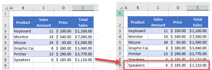
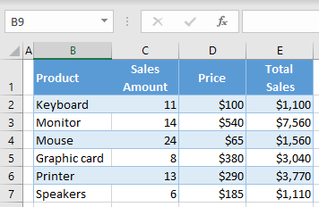
Say you have the following data set and want to copy Row 7 to Row 8.

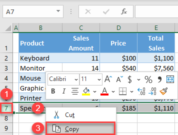
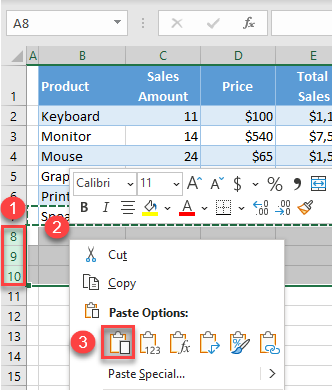
Select the row you want to copy by clicking on a row number (here, Row 7), then right-click anywhere in the selected area and choose Copy (or use the keyboard shortcut CTRL + C).

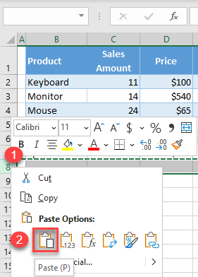
Right-click the row number where you want to paste the copied row and click Paste (or use the keyboard shortcut CTRL + V).

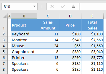
As a result, the entire Row 7 is copied to Row 8.

To use copy and paste to duplicate a whole row within a macro, see VBA Copy / Paste Rows & Columns.

Copy a Row to Multiple Rows

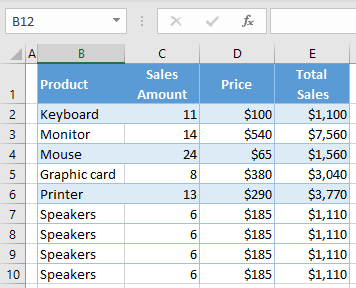
You can also copy one row and paste it into multiple rows. For example, follow these steps to copy Row 7 to Rows 8–10:

Select the row you want to copy by clicking on a row number (Row 7). Then right-click anywhere in the selected area and choose Copy (or use the keyboard shortcut CTRL + C).

Select the row numbers where you want to paste copied row, then right-click anywhere in the selected area, and choose Paste (or use the keyboard shortcut CTRL + V).

As a result, Row 7 is now copied to Rows 8–10.

Duplicate Rows With the Fill Handle

You can also duplicate rows using the fill handle.

Select the row you want to copy, and position the cursor in the bottom-left corner of the selection range until the small black cross appears (the Fill Handle).

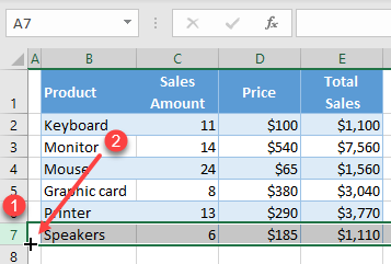
Then drag the cursor down to the next row (or to multiple rows, depending on the number of duplicates you want).

The result is exactly the same as demonstrated with the copy and paste method above.

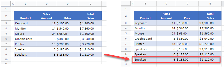
Duplicate Rows in Google Sheets

You can use any of the options above in exactly the same way in Google Sheets to duplicate rows.

Источник

Download PC Repair Tool to quickly find & fix Windows errors automatically

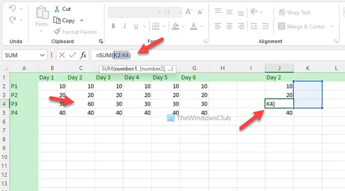
If you need to cut-paste or copy-paste Columns and Rows in an Excel spreadsheet, you can try out this method mentioned in the article. This guide helps you to copy multiple columns and rows along with the formulas you inserted in any particular cell.

Let’s say that you have a spreadsheet with multiple rows and columns. You need to move some rows or columns from one place to another to match something in the sheet. When you move a column, the associated formulas do not move alongside. However, this guide will help you to move a column or row along with the formula. Although it is not possible to cut or copy a row or column along with the applied formula, you can identify the cells and apply the same formula again.

To Copy Paste columns and rows in Excel spreadsheet, follow these steps:

Open an Excel spreadsheet on your computer.
Select a row or column you want to copy or cut.
Press the Ctrl+Cto copy or Ctrl+X to cut.
Select the destination row or column where you want to paste it.
Press the Ctrl+Vto paste the data.
Click on the cell to change the formula.
Click on the top formula bar and write down the new formula.
Press the Ctrl+Sto save the changes.

To learn more about these steps, continue reading.

To get started, you need to open the Excel spreadsheet on your computer and select a row or column you want to cut or copy to another location.

You have two options to cut or copy the row and column. You can either use the Ctrl+C or Ctrl+X keyboard shortcut or right-click on the row/column and choose the Copy or Cut option.

After that, select the desired row or column where you want to paste the data. Then, press the Ctrl+V keyboard shortcut to paste the copied content to the selected row or column.

Now, your data is pasted, but the formulas are messed up. You need to click on a particular cell where you used a formula earlier, click on the formula bar on the top of the spreadsheet, and edit the formula accordingly.

At last, click on the Ctrl+S to save all the changes.

Note: If you do not change the formula after pasting the data to the new row or column, it will not show the correct information in the new place. Simple as well as complex formulas do not get changed as you change the row or column. The second important thing is that your selected rows and columns should not contain any chart.

How do I copy multiple rows and columns to another sheet in Excel?

To copy multiple rows and columns to another sheet in Excel, you do not need to do anything special. That said, you can open the source spreadsheet first, select the rows and columns, and press the Ctrl+C buttons together to copy. Then, you can open the second spreadsheet and press the Ctrl+V to paste the content.

Can you Copy and paste whole columns in Excel?

Yes, you can copy and paste whole columns in Excel. There is nothing special in doing so. Having said that, you can select the columns you want to copy and press the Ctrl+C buttons. Then, you can open another spreadsheet and press the Ctrl+V to paste.

That’s all! Hope it helped.

Read: How to create Custom Excel FunctionsThat’s all! Hope this guide helped.

Ezoic

When he is not writing about Microsoft Windows or Office, Sudip likes to work with Photoshop. He has managed the front end and back end of many websites over the years. He is currently pursuing his Bachelor’s degree.

Источник

If you’re looking for a way to move rows of data from one sheet to another depending on the value in a given cell, there’s, unfortunately, no direct feature or menu item for it on Excel.

However, there are some ways that we can suggest for you to get this done.

In this tutorial we will show you two ways to move a row to another sheet based on cell value in Excel:

Using Excel filters
Using a simple VBA Macro

There are two ways to move rows to another sheet based on a cell value.

The first method is a more manual method, that involves the use of filters to extract the rows that match a given cell value.

You can then select these extracted values, copy and manually paste them to your required worksheet.

The second method involves the use of a VBA script that automatically moves the rows to your required sheet instantly whenever it matches a given cell value.

For both methods, we will consider the following dataset:

Each row in this dataset contains details about a single client.

The last cell of each row contains the status of transactions with the client. So if a deal with a client is pending, the Status will be ‘Pending’.

Now, we want that when a deal with a given client is ‘Closed’, the client’s details (or the row containing the client’s details) is moved to a separate sheet, say Sheet2.

Dataset where some records status is closed

Let us take a look at the two ways in which we can accomplish this.

Using Filters to Move Row to another Sheet based on Cell Value in Excel

Excel filters are used to extract records that match the specified criteria.

So they can be really helpful when you want to display the matching records of your data while hiding the others.

To use filters on our sample dataset, follow the steps below:

Select the entire dataset.
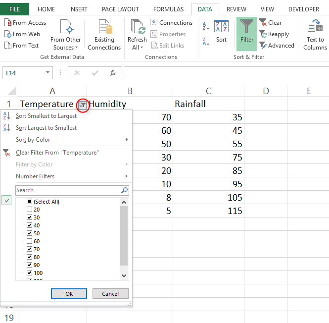
Click the Data tab
Click on the Filter icon (under the ‘Sort and Filter’ group).

You will see that all the header cells now have a small downward pointing arrows. Click on the arrow next to the Status header.

From the dropdown that appears, make sure that only the box next to “Closed” is checked.

Click OK. You will now see only the rows where the Status is “Closed”.

Select all the rows in view (except the header row) and press Alt+; (Cmd+Shift+Z on a Mac) so that only the visible rows are selected.
Right-click and select “Copy” from the popup menu, or simply press CTRL+C on the keyboard..This will copy all the visible rows only.
Select the tab corresponding to the new worksheet (Sheet2 in our example), and paste it there by pressing CTRL+V.

Copy and Paste these records into another sheet

Return to your original worksheet and right click on the selected visible rows.Click on the Delete option.This will remove the visible rows from the current worksheet (Sheet1).

Click on the Filter button from the Data tab once again to remove the filters.

You should now see all your data, without the rows corresponding to any “Closed” clients.

Note that this whole process is partially manual since you have to physically copy and paste the filtered out rows to the new sheet.

Moreover, the process does not happen in real-time.

So in case you add a new record where the client status is closed, you will have to repeat the entire process and manually copy the filtered rows into the other sheet.

I know this is not the best way, but it’s fast and gets the work done. Use this method if you have a dataset that doesn’t update (so you only have to do this once or a few times at best).

Also note that in this example, I have only used the cell value in one column (the status column). You can also do this for multiple cell values. For example, move all the clients where status is closed and the region in North America. For this, you simply need to apply two filters and then copy and paste the records.

In the above example, we have copied the records to another sheet, so these records still remain in the original dataset. In case you want these to move completely (i.e., not be a part of the original dataset), instead of copy-paste, use cut-paste.

Now, if you can handle a little bit of VBA and automation, let me show another way to move rows to a separate sheet based on the cell value.

Using VBA to Move Row to another Sheet based on Cell Value in Excel

A second, and more efficient way to move a row to another sheet based on cell value is by using a simple VBA macro code.

In this section, we will provide a few lines of Excel VBA code to help you accomplish this.

We will also explain the code and how it works so that you can customize it to your own requirement.

Suppose you have a dataset shown below and you want to move all the records where the status is ‘Closed’ to another sheet.

I will cover two scenarios in this section:

VBA code to Move a row to another sheet and delete it from the original dataset
VBA code to Move a row to another sheet and also keep it in the original dataset

VBA Code (Move Row to Another Sheet & Delete From Original Data)

Here’s the code that we are going to use:

'VBA Code by Scott from SpreadsheetPlanet.com
Sub move_rows_to_another_sheet()
For Each myCell In Selection.Columns(4).Cells
If myCell.Value = "Closed" Then
myCell.EntireRow.Copy Worksheets("Sheet2").Range("A" & Rows.Count).End(3)(2)
myCell.EntireRow.Delete
End If
Next
End Sub

This code will copy the entire row corresponding to a cell value containing the word ‘Closed’’ into the worksheet named ‘Sheet2’. Also, the records where the status is closed will be deleted from the original dataset.

To run this code

If your worksheet name is something else, you can change the VBA code (change the name of the sheet in the 4th line of the code)

The moved row will be pasted right after the current last row in the destination sheet.

VBA Code (Move Row to Another Sheet & Keep in Original Data)

While the above code would move all the records whether status is closed and also delete it from the original data set, below is the code that would not delete the data from the original data set

'VBA Code by Scott from SpreadsheetPlanet.com
Sub move_rows_to_another_sheet()
For Each myCell In Selection.Columns(4).Cells
If myCell.Value = "Closed" Then
myCell.EntireRow.Copy Worksheets("Sheet2").Range("A" & Rows.Count).End(3)(2)
End If
Next
End Sub

The only change I have done here is deleted the following line of code:

myCell.EntireRow.Delete

Now that I have given you the VBA code for both the scenarios, let me show you where to put this code and how to run it,

Where to Put the VBA code

To use the above code, all you need to do is copy and paste it into the VBA window.

Here’s how:

Click the Developer option in the ribbon
Click on Visual Basic. Ths will open the VBA window
In VBA backend that opens, you will see all your project files and folders in the Project Explorer on the left side.
From the Insert Menu, select the Module option.

This will open up a new module window for your selected sheet.
Now you can start coding. Copy the above lines of code and paste them into the blank module window.

Copy-paste the code in the module window

Close the VBA window.

Running the Macro

Now that your macro is ready, you can go ahead and run it.

Select the area containing your data in the original worksheet.

In our example, select the range A2:D11 of Sheet1.

Next, select Macros from the Developer menu.

This will open the Macro dialog box. Select the Macro Name: move_rows_to_another_sheet and click Run.

Select the macro name in the Macro dialog box

If you used the first code (that deletes the record that is moved), your final data would look like this:

Notice that the rows corresponding to “David Jones” and “Cierra Vega” are gone, since they had the Status=”Closed”.

The two rows that have been removed from Sheet1 should now have moved to Sheet2:

Rows have been moved to the destination sheet

Explanation of the Code

Let us take a few minutes to understand this code so that you can customize it according to your requirement.

The code loops through each cell in column “4” (or column D) of the worksheet:

For Each myCell In Selection.Columns(4).Cells

If a cell contains the value “Closed”, then we copy the entire row corresponding to that cell into Sheet2 (in column A, and the row after the last row in the sheet).

If myCell.Value = “Closed” Then
myCell.EntireRow.Copy Sheet2.Range(“A” & Rows.Count).End(3)(2)
We then delete the copied row from Sheet1
myCell.EntireRow.Delete

Note: If you would rather just send a copy of the rows to Sheet2, without deleting them from Sheet1, then you can simply omit this line from the code.

You can go ahead and adjust this code according to your dataset. Simply replace Column number 4 (in line 2) with the column number you need to analyze and replace the value “Closed” (in line 3) with the cell value you need as your qualifier for moving rows.

You can also change the sheet name from “Sheet2” (in line 4) to the name of your destination sheet.

In this tutorial, I showed you how to use a simple Filter technique and a simple VBA macro code to move rows to another sheet based on a cell value.

While the first method is more manual, the second method uses a VBA code that makes is automatic and a lot faster.

With the VBA code, you can simply select the range of cells containing your data and have all the rows containing a particular cell value moved to a different sheet by running a macro.

Happy coding!

Other Excel tutorials you may also like:

How to Hide Rows based on Cell Value in Excel
How to Remove Duplicate Rows based on one Column in Excel?
How to Hide Columns Based on Cell Value in Excel
How to Select Rows with Specific Text in Excel
How to Select Multiple Rows in Excel
How to Delete Filtered Rows in Excel (with and without VBA)

Источник

See also

​Copy rows to the destined sheet based on column criteria.

Duplicate Rows – Copy and Paste

Copy a Row to Multiple Rows

Duplicate Rows With the Fill Handle

Duplicate Rows in Google Sheets

How do I copy multiple rows and columns to another sheet in Excel?

Can you Copy and paste whole columns in Excel?

Using Filters to Move Row to another Sheet based on Cell Value in Excel

Using VBA to Move Row to another Sheet based on Cell Value in Excel

VBA Code (Move Row to Another Sheet & Delete From Original Data)

VBA Code (Move Row to Another Sheet & Keep in Original Data)

Where to Put the VBA code

Running the Macro

Explanation of the Code

Copy rows to the destined sheet based on column criteria.