
Copying files in excel is an important skill that you need as a student or a business person. It is necessary for an individual in this modern technological era to learn copying file name in excel. It is one of the most useful skill in the world.
The copy file name option in Excel is a useful way to display chunk of files in excel or make changes to the name of a file. If you want to copy large number of file names into excel, it will be a hectic and tedious task if you type them manually. In this article we will show you how copy file names in excel in easy and simple way. There are different methods to do it. Let us take you through to each one by one.
Tips that are provided in this article are compatible with versions 2010/2013/2016.
USING CTRL+C AND CTRL+V TO COPY FILE NAMES IN EXCEL
If you want to copy the name of a file in Excel, use CTRL+C and CTRL+V. The keyboard shortcut is Ctrl+c, followed by Ctrl+v on your PC or Command+c followed by Command+v on Mac.
This works well if you want to paste the copied name into another column or cell of your workbook. For example, if you want to copy a filename from one sheet and paste it into another sheet, then use ctrl-c followed by ctrl-v.
1. Open Excel as well as file explorer Open File Explorer
2. Select the file you want to copy.
3. Press CTRL+C
4. Paste the file by using CTRL+V on Excel sheet.
USING COPY AS PATH TO COPY FILE NAMES IN EXCEL
Copy as Path is used to create shortcuts on the desktop and in the Start menu. It is very useful when you want to create shortcuts for files or folders that are located at different locations on your computer.. You can also use this to copy file names into excel.
To copy a file name in Excel, you can use the following steps:
1. Open Excel.
2. Navigate to the folder and select the required files.
3. Right click the mouse, a window will pop up. In this window, select copy as path. This copy the path of files to clipboard.
4. Navigate to excel, press the ALT + TAB key, and paste the files.
And that’s it , you have copied file names into the excel
Copying File name in Excel using Import data
1. Click on Data > Import Data > From File > Select data source.
2. Enter the main folder of your files and select the files you want to import
3. Select open and your file name is copied into excel.
That’s how you import files into excel by using in built tools
Did you learn about how to copy file names in excel using different methods. You can follow WPS academy to learn more features of Word document, Excel Spread sheets, and power point slides.
You can also download WPS office to edit the word documents , Excel Spread sheets, and PowerPoint free of cost. Download Now! And get an enjoyable working space.
In this short post, I’m going to show you how to easily copy all filenames in a Window folder to Microsoft Excel.
First a caveat, the main limitation of the method I’m going to show you, is that you cannot copy filenames in subfolders. If you want to learn how to how to copy filenames in subfolders, check out the how to easily copy all filenames in a folder to Excel using CMD post.
Let’s jump right into it.
Step 1: Open Excel
Open up excel and then navigate to the folder that contains the files.

Step 2: Navigate to Folder and Select All the Files
Navigate to the folder that contains the files. In the folder that contains the files, select all the files in the folder. You can use the shortcut keys, Ctrl + a.

Step 3: Hold Shift Key and Right Click
Now, holding the Shift key, hover over your selection and right click. Don’t let go of the Shift key before you right click.

Step 4: Click Copy as Path
In the window that pops up, click copy as path. This copies the file path of all the files to the Clipboard.

Step 5: Paste Filepaths in Excel
Navigate to Excel, I’m using ALT and Tab key, and paste the file paths.

Step 6: Use Replace Function in Excel
We are going to remove the folder path using replace function in excel and we’ll have the filenames.
So double click on one of the cells, select and copy the folder path. Click on Find and Select, scroll down to replace. Click on replace and paste the folderpath. Then click on replace all.
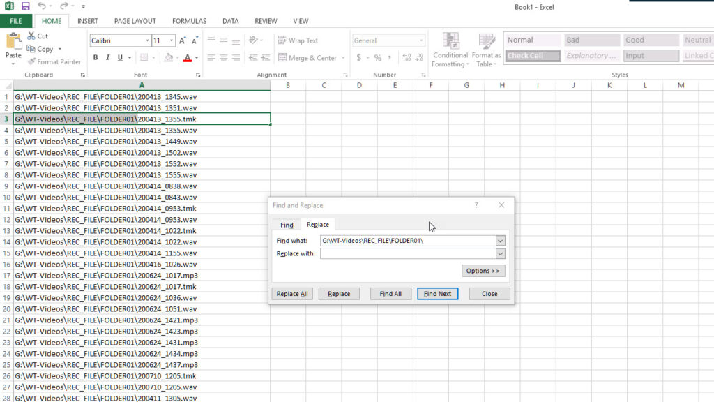
Close the Find and Select dialog. Save your excel document and you have successfully copied all the file names in a folder into an excel document.
That’s it for this post, if you want to learn how to also copy the filenames into text check out this post on how to copy file names in windows explorer to text.
And here’s a short how-to video:
See all How-To Articles
This tutorial will demonstrate how to paste range names in Excel.
If you have a workbook that contains a lot of named ranges, you can use those range names in alternative locations or formulas in your Excel file.
Pasting a Range Name to Another Location
- First, select the cell where you wish the range name to be pasted.
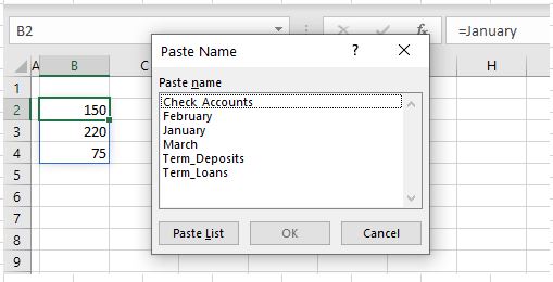
- In the Ribbon, select Formulas > Defined Names > Use in Formula > Paste Names…
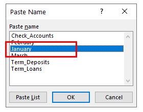
- Select the name you want to paste, then click OK.
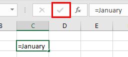
- Press the ENTER key on the keyboard or click the check mark in the formula bar.
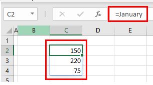
The range name will be inserted as a Dynamic Array. You cannot edit individual cells in a dynamic array or delete the values in the cells underneath your formula (for example the values in C3 and C4 in the example below): The cells, together, form part of an individual range name.
Pasting a Range Name into a Formula
You can also paste range names into formulas.
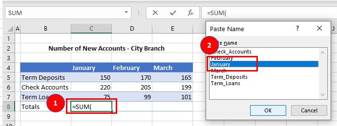
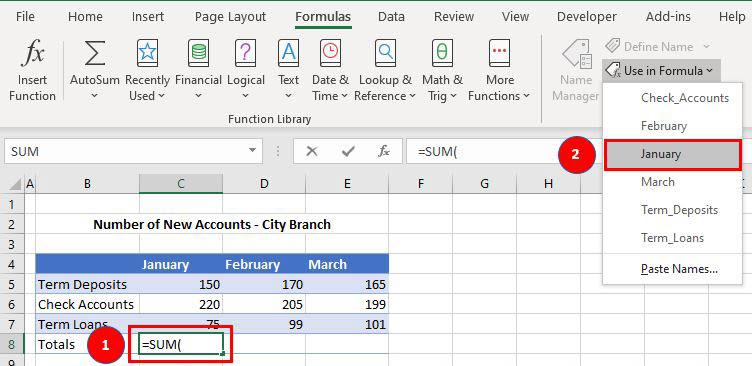
- First, type the beginning of the formula. (This example uses the SUM Function.)
- In the Ribbon, go to Formulas > Defined Names > Use in Formula > Paste Names… Then select the name required and click OK.
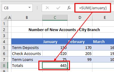
- Press ENTER for Excel to automatically complete the formula with a closing parenthesis.
Use in Formula List
An alternative (and simpler!) way to paste a range name into a formula is to directly select the name from the Use in Formula list.
- Type the first part of the formula.
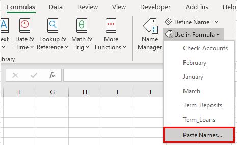
- In the Ribbon, go to Formulas > Defined Names > Use in Formula, then select the name you require.
- Press ENTER for Excel to automatically complete the formula with a closing parenthesis.
Copying and pasting is a very frequently performed action when working on a computer. This is also true in Excel.
It’s so common that almost everyone knows the keyboard shortcuts to copy Ctrl + C and paste Ctrl + V.
When using this in Excel, it will copy everything including values, formulas, formatting, comments/notes, and data validation.
This can be frustrating as sometimes you’ll only want the values to copy and not any of the other stuff in the cells.
In this post, you’ll learn all the ways to copy and paste only the values from your Excel data.
Example Data
The example data used in this post contains various formatting.
- Cell formatting such as font color, fill color, number formatting, and borders.
- Notes.
- SUM formula.
- A data validation dropdown list.
Paste Special Keyboard Shortcut
If you want to copy and paste anything other than an exact copy, then you’re going to need to become familiar with paste special.
A favorite method to use this is with a keyboard shortcut.
To use the paste special keyboard shortcut.
- Copy the data you want to paste as values into your clipboard.
- Choose a new location in your workbook to paste the values into.
- Press Ctrl + Alt + V on your keyboard to open up the Paste Special menu.
- Select Values from the Paste option or press V on your keyboard.
- Press the OK button.
This will paste your data without any formatting, formulas, comments/notes, or data validation. Nothing but the values will be there.
Paste Special Legacy Keyboard Shortcut
This keyboard shortcut is a legacy shortcut from before the Excel ribbon command existed and it’s still usable.
In fact, when you try and use this you’ll be greeted with the above warning to let you know this is from an earlier version of Microsoft Office.
When you have a range of data copied to your clipboard, you can open up the Paste Special menu by pressing Alt + E + S on your keyboard.
Once the Paste Special menu is open you can then press V for Values.
One advantage the legacy shortcut has is it can easily be performed with one hand!
Paste Special Values Keyboard Shortcut
Pasting as values is a very common activity in Excel. Because of this, a new keyboard shortcut was introduced to Microsoft 365 users for this exact purpose.
Press Ctrl + Shift + V on your keyboard to paste the last item in your clipboard as values.
This is the most useful new shortcut as it bypasses the paste special menu entirely.
Paste Special from the Home Tab
If you’re not a keyboard person and prefer using the mouse, then you can access the Paste Values command from the ribbon commands.
Here’s how to use Paste Values from the ribbon.
- Select and copy the data you want to paste into your clipboard.
- Select the cell you want to copy the values into.
- Go to the Home tab.
- Click on the lower part of the Paste button in the clipboard section.
- Select the Values clipboard icon from the paste options.
The cool thing about this menu is before you click on any of the commands you will see a preview of the data you’re about to paste. This makes it easy to ensure you’re selecting the right option.
Paste Values with Hotkey Shortcuts
Since the paste values command is in the ribbon, that also means you can access it with the Alt hotkeys.
Notice when you press the Alt key, the ribbon lights up with all the accelerator keys available.
Pressing Alt ➜ H ➜ V ➜ V will activate the paste values command.
Paste Values from Right Click Menu
Paste Values is also available from the right-click menu.
Copy the range of cells you want to paste as values ➜ right click ➜ select the paste values clipboard icon.
Paste Values with Quick Access Toolbar Command
If it’s a command you use quite frequently, then why not put it in the quick access toolbar?
This way it’s only a click away at all times!
Depending on where in the quick access toolbar you place it, it will also get its own easy to use Alt hotkey shortcut too.
Check out this post for details on how to add commands to the quick access toolbar, or this post on other interesting commands you can add to the quick access toolbar.
You can add the paste values command from the Excel Options screen.
- Select All Commands from the dropdown list.
- Locate and select Paste Values from the options. You can press P on your keyboard to quickly navigate to commands starting with P.
- Press the Add button.
- Use the Up and Down arrows to change the ordering of commands in your toolbar.
- Press the OK button.
The command will now be in your quick access toolbar!
If you place it in the 4th position like in this Example, then you can you Alt + 4 to access it with a keyboard shortcut.
Paste Values Mouse Trick
There’s a mouse option you can use to copy as values which most people don’t know about.
- Select the range of cells to copy.
- Hover the mouse over the active range border until the cursor turns into a four directional arrow.
- Right-click and drag the range to a new location.
- When you release the right click, a menu will pop up.
- Select Copy Here as Values Only from the menu.
This is such a neat way, and there are a few other options in this hidden menu that are worth exploring.
Paste Values with Paste Options
There’s another sneaky method to paste values.
When you do a regular copy and paste, a small icon will appear in the bottom right corner of the pasted range. It will remain there until you interact with something else in your spreadsheet.
These are the paste options and you can click on it or press Ctrl to expand the options menu.
When you open the menu, you can then either click on the Values icon or press V to change the range into values only.
Paste Values and Formulas with Text to Columns
I don’t really recommend using this method, but I’m going to add it just for fun.
A few caveats with this method.
- You can only copy and paste one column of data.
- It will keep any formulas.
- It will remove the formatting, comments, notes, and data validation.
If that’s exactly what you’re looking for, then this method might be of interest.
Select a single column of data ➜ go to the Data tab ➜ select the Text to Column command.
This will open up the Convert Text to Column Wizard. In the first step, you can select Delimited and press the Next button.
You can also select Fixed width as we won’t be using the text to column functionality it doesn’t really matter.
In the next step, remove any selected delimiters and press the Next button.
In the last step, select the destination cell for the output and press the Finish button.
You can see the results have all the formatting gone but any formulas still remain.
Paste Values with Advanced Filters
This one is another not-quite paste values option and is listed for fun as well.
It will remove any formulas, comments, notes, and data validation but will leave all cell formatting.
With your data selected go to the Data tab then select the Advanced command in the Sort and Filter section.
From the Advanced Filter Menu.
- Select Copy to another location.
- Leave the Criteria range empty.
- Select a location to place the copied data.
- Press the OK button.
This will create a copy of the data as values and remove any formulas, comments, notes, and data validation.
You can then remove the cell formatting that’s left by going to the Home tab ➜ Clear ➜ and selecting the Clear Formats option.
Conclusions
Wow! That’s a lot of different ways to paste data as values in Excel.
It’s understandable there are so many options given it’s an essential action to avoid carrying over unwanted formatting.
You’re eventually going to need to do this and there are quite a few ways to get this done.
What’s your favorite way? Did I miss any methods you use? Let me know in the comments!
About the Author
John is a Microsoft MVP and qualified actuary with over 15 years of experience. He has worked in a variety of industries, including insurance, ad tech, and most recently Power Platform consulting. He is a keen problem solver and has a passion for using technology to make businesses more efficient.
Asked
12 years, 11 months ago
Viewed
3k times
Is there a way to copy a cell that also has a «name», and paste it somewhere else so that the new cell also has the same «name»?
![]()
asked May 14, 2010 at 20:44
0
This VBA code copies all the nakms from active workbook to destination. Not quite sure what your trying to do but this should get you started:
Sub Copy_All_Defined_Names()
   ' Loop through all of the defined names in the active
   ' workbook.
     For Each x In ActiveWorkbook.Names
      Workbooks("Destination.xls").Names.Add Name:=x.Name, _
         RefersTo:=x.Value
   Next x
End Sub
From here:
http://support.microsoft.com/kb/213389
answered May 14, 2010 at 21:18
![]()
1
Home > Data Recovery > 2 Methods to Copy the List of All File Names in a Folder into Your Excel Worksheet
Sometimes you will need to list all the file names in a folder in an Excel worksheet. Thus, you can better manage those files. In this article, we will introduce two effective methods to copy the list in a folder.
In an Excel worksheet, you can make a menu of some important files. And you need to copy the list of all the file names into one worksheet. However, when there are hundreds or thousands of files, you will find it hard to do this. In the image below, you can see several files.
Now you need to copy the list of all the file names into a worksheet in another Excel file. If you copy and paste them one by one manually, you will certainly spend a lot of time and energy. At this time, you can use the two methods below.
Method 1: Use a New Text Document
Now follow the steps below and see how this method takes effect.
- Before you perform this process, make sure that you have shown the file extensions in your computer. Click the button “Start” in your computer.
- And then click the button “Control Panel”.

- In the control panel, click the “Appearance”.
- And then click the button “Folder Options”.
- After that, choose the option “View” in the “Folder Options” window.
- Next uncheck the option “Hide extension for known file types”.
- And then click “OK” to save the setting.


Therefore, you can see all the extensions of files in your computer.
- Come back to the folder, create a new text document and give it a new name. We will name it “DataNumen Sales Volume”.
- And then open this text file.
- After that, input the following characters into this file:
dir> 1.txt

- Next save this file and close it.
- In this step, change the extension of this file from “.txt” into “.bat”.
- After that, you will see a new window pop up. Here you need to click the button “Yes” to confirm this change.

- And then double click this file again. Next you will see a new text document with the name “1” in this folder.
- Open this new text document in this folder. You will see all the name information in it.
- After that, copy the necessary part in this file.

- And then in the target worksheet, click the small arrow under the button “Paste”.
- In the drop-down list, choose the option “Use Text Import Wizard”.

- Next in the new window, choose the option “Fixed width”.
- And then click the button “Next”.

- In step 2 of the wizard, move the break line and make sure that the names of those files will be in one cell.
- And then also click “Next”.

- In step 3, click “Finish”. Thus, all the information will appear in the worksheet.


You can delete the other useless columns in the worksheet. By using this method, you don’t have to copy and paste the names one by one.
Method 2: Define Name
In this part, we will introduce another excellent method.
- Click the tab “Formulas” in the ribbon.
- And then click the button “Define Name”.
- In the “New Name” window, input a name into the first text box. We will also name it “DataNumen_Sales_Volume”.
- After that, input this formula into the “Refers to” text box:
=FILES(“C:UsersSampleDesktopSales Volume*.*”) &T(NOW())
The path of the folder is “C:UsersSampleDesktopSales Volume” in this example. You need to change it into your actual folder path.
- And then click the button “OK” in the window.
- Now input the following formula into one cell in the worksheet:
=IF(ROW(A1)>COUNTA(DataNumen_Sales_Volume),””,INDEX(DataNumen_Sales_Volume,ROW(A1)))
In this formula, you need to change the define name into yours.
- After that, click the fill handle of this cell and drag downwards. As you move your mouse, you will also find that all the names will appear in this column.

- But you may also find that those results are the results of formulas. You still need to copy and paste them as texts.
- Next delete the formulas in the worksheet.

Until now, you have gone through all the steps. This method is also very effective for this requirement.
A Comparison of the Two Methods
You can see that both of the two methods are very useful. Here we will compare the two methods in this part.
|
Comparison |
Use a New Text Document |
Define Name |
|
Advantages |
If you are not familiar with Name and the complex formula in cells, you can use this first method. | There are fewer steps in this method. You can finish your tasks quickly by using it. |
|
Disadvantages |
Compared with the second methods, there are more steps in this method. You still need to spend a lot of time. | The formulas in cells will produce the results that you need. Therefore, you still need to copy and paste them as values. |
When you need to input all file names into a worksheet, you will know which method is the most suitable one.
Take Actions Quickly in a Data Disaster
It is unavoidable that you will meet with data disaster. In such an accident, your Excel files will most possibly be damaged. Therefore, you need to take actions quickly. In order to repair corrupt xls data quickly and safely, you can use out excellent Excel repair tool. This tool is able to fix most of the Excel problems.
Author Introduction:
Anna Ma is a data recovery expert in DataNumen, Inc., which is the world leader in data recovery technologies, including repair Word doc data error and outlook repair software products. For more information visit www.datanumen.com
Looking for a primer on how to create and work with names in Microsoft Office Excel? You’ve come to the right place. In this free video tutorial from everyone’s favorite MS Excel guru, YouTube’s ExcelIsFun, the 12.66th installment in his series of Excel name tricks, you’ll learn how to paste a list of all names in the workbook, both the name and the formula that defines the name.
Want to master Microsoft Excel and take your work-from-home job prospects to the next level? Jump-start your career with our Premium A-to-Z Microsoft Excel Training Bundle from the new Gadget Hacks Shop and get lifetime access to more than 40 hours of Basic to Advanced instruction on functions, formula, tools, and more.
Buy Now (97% off) >
Other worthwhile deals to check out:
- 97% off The Ultimate 2021 White Hat Hacker Certification Bundle
- 98% off The 2021 Accounting Mastery Bootcamp Bundle
- 99% off The 2021 All-in-One Data Scientist Mega Bundle
- 59% off XSplit VCam: Lifetime Subscription (Windows)
- 98% off The 2021 Premium Learn To Code Certification Bundle
- 62% off MindMaster Mind Mapping Software: Perpetual License
- 41% off NetSpot Home Wi-Fi Analyzer: Lifetime Upgrades