Copy from one cell to another excel

Move or copy cells and cell contents

Use Cut, Copy, and Paste to move or copy cell contents. Or copy specific contents or attributes from the cells. For example, copy the resulting value of a formula without copying the formula, or copy only the formula.

When you move or copy a cell, Excel moves or copies the cell, including formulas and their resulting values, cell formats, and comments.

You can move cells in Excel by drag and dropping or using the Cut and Paste commands.

Move cells by drag and dropping

1. Select the cells or range of cells that you want to move or copy.

2. Point to the border of the selection.

3. When the pointer becomes a move pointer , drag the cell or range of cells to another location.

Move cells by using Cut and Paste

1. Select a cell or a cell range.

2. Select Home > Cut or press Ctrl + X.

3. Select a cell where you want to move the data.

4. Select Home > Paste or press Ctrl + V.

Copy cells by using Copy and Paste

1. Select the cell or range of cells.

2. Select Copy or press Ctrl + C.

3. Select Paste or press Ctrl + V.

Need more help?

You can always ask an expert in the Excel Tech Community or get support in the Answers community.

See Also

Move or copy cells, rows, and columns

See all How-To Articles

This tutorial demonstrates how to copy data from one cell to another automatically in Excel.

Copy Data Automatically

To copy and paste data from one cell to another in your current worksheet, you can create a VBA macro.

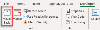
1. In the Ribbon, go to Developer > Visual Basic. If you don’t have this tab available, find out how to add the Developer tab.

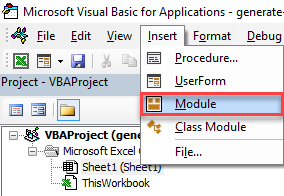
1. In the VBA window, in the Menu, select Insert > Module.

1. In the code window on the right side, type the following macro:

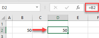
Sub CopyData()
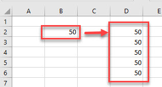
   Range("B2").Copy Range("D2")
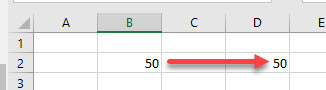
End Sub

This copies the data that is in cell B2 to cell D2.

1. You can extend this macro to copy to more than one cell.

Sub CopyData()
   Range("B2").Copy Range("D2:D6")
End Sub

This copies the data in cell B3 across to D2 and down to D6.

ActiveCell

In the two macros above, you do not have to have cell B2 selected in order to copy the data as the range is specified in the macro. If, however, the macro uses the ActiveCell property, then you would need to select the cell with data you want to copy before running the macro.

Sub CopyData()
   ActiveCell.Copy Range("D2")
End Sub

Note: You can also use VBA code for many other copy and paste options in Excel.

Create a Formula in VBA to Copy Data

You can also copy data automatically in Excel using a formula. You can create the formula manually, or use VBA.

Sub CreateFormula()
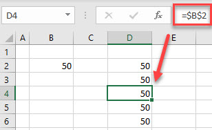
   Range("D2") = "=B2"
End Sub

Or use a macro to copy a cell to a range of multiple cells. However, due to the nature of Excel – that it copies formulas relative to each cell address – make sure you anchor the cell in place using absolute addressing.

Sub CreateFormula()
   Range("D2:D6") = "=$B$2"
End Sub

The formula would then be copied down from cell D2 to D6.

Here’s a VBA in a simple form. Just create a macro, add these lines to it. Then select your original column (what you’re calling column 1), and run the macro.

a = ActiveCell.Value
b = ActiveCell(1, 2).Value

ActiveCell.Value = a + b

The bracketed cell reference is a relative statement — 1, 2 means «same row, one column to the right» so you can change that if you need. You could make it loop by expanding thusly:

Do
a = ActiveCell.Value
b = ActiveCell(1, 2).Value

ActiveCell.Value = a + b

ActiveCell.Offset(1, 0).Select

If ActiveCell.Value = "" Then
    Exit Do
End If
Loop

That loop will carry on until it finds a blank cell, then it’ll stop. So make sure you have a blank cell where you want to stop. You could also add extra characters into the line that combines.. so in the above example it’s ActiveCell.Value = a + b, but you could make it ActiveCell.Value = a + " - " + b or anything else that may help.

No. There is no ‘easier’ way. If you want to put the contents of A1 (e.g. abc) into the contents of B1 (e.g. 123456) so that B1 will then contain 123abc456 then you have to use F2 (or double-click for ‘In-Cell editing’) to select and capture/copy the content from A1.

However, if the position of the content of the paste is static (i.e. doesn’t change) then you could macro it. For example, if you wanted to put anything you type into a cell in column A as a new line (i.e. paragraph) to the content of the cell in column B in the same row, right-click the worksheet’s name tab and choose View Code then paste this into the worksheet’s code sheet.

Option Explicit

Private Sub Worksheet_Change(ByVal Target As Range)

    If Not Intersect(Range("A:A"), Target) Is Nothing Then

        On Error GoTo bye
        Application.EnableEvents = False
        Dim t As Range, b As String

        For Each t In Intersect(Range("A:A"), Target)

            b = vbNullString 

            If t.Offset(0, 1).Value <> vbNullString Then
                b = t.Offset(0, 1).Text & Chr(10)
            End If

            If t.Value <> vbNullString Then
                t.Offset(0, 1) = b & t.Text
            End If

        Next t

    End If

bye:
    Application.EnableEvents = True

End Sub

Anything you type into column A will appear at the end of the content in column B on the same row.

Copying and Pasting a cell or a range of cells is one of the most common tasks users do in Excel.

A proper understanding of how to copy-paste multiple cells (that are adjacent or non-adjacent) would really help you be a lot more efficient while working with Microsoft Excel.

In this tutorial, I will show you different scenarios where you can copy and paste multiple cells in Excel.

If you have been using Excel for some time now, I’m quite sure you would know some of these already, but there’s a good chance you’d end up learning something new.

So let’s get started!

Copy and Paste Multiple Adjacent Cells

Let’s start with the easy scenario.

Suppose you have a range of cells (that are adjacent) as shown below and you want to copy it to some other location in the same worksheet or some other worksheet/workbook.

Below are the steps to do this:

1. Select the range of cells that you want to copy

1. Right-click on the selection
2. Click on Copy

1. Right-click on the destination cell (E1 in this example)
2. Click on the Paste icon

The above steps would copy all the cells in the selected range and paste them into the destination range.

In case you already have something in the destination range, it would be overwritten.

Excel also gives you the flexibility to choose what you want to paste. For example, you can choose to only copy and paste the values, or the formatting, or the formulas, etc.

These options are available to you when you right-click on the destination cell (the icons below the paste special option).

Or you can click on the Paste Special option and then choose what you want to paste using the options in the dialog box.

Useful Keyboard Shortcuts for Copy Paste

In case you prefer using the keyboard while working with Excel, you can use the below shortcut:

• Control + C (Windows) or Command + C (Mac) – to copy range of cells
• Control + V (Windows) or Command + V (Mac) – to paste in the destination cells

And below are some advanced copy-paste shortcuts (using the paste special dialog box).

To use this, first copy the cells, then select the destination cell, and then use the below keyboard shortcuts.

• To paste only the Values – Control + E + S + V + Enter
• To paste only the Formulas – Control + E + S + F + Enter
• To paste only the Formatting – Control + E + S + T + Enter
• To paste only the Column Width – Control + E + S + W + Enter
• To paste only the Comments and notes – Control + E + S + C + Enter

In case you’re using Mac, use Command instead of Control.

Also read: How to Cut a Cell Value in Excel (Keyboard Shortcuts)

Mouse Shortcut for Copy Paste

If you prefer using the mouse instead of the keyboard shortcuts, here is another way you can quickly copy and paste multiple cells in Excel.

1. Select the cells that you want to copy
2. Hold the Control key
3. Place the mouse cursor at the edge of the selection (you will notice that the cursor changes into an arrow with a plus sign)
4. Left-click and then drag the selection where you want the cells to be pasted

This method is also quite fast but is only useful in case you want to copy and paste the range of cells in the same worksheet somewhere nearby.

If the destination cell is a little far off, you’re better off using the keyboard shortcuts.

Copy and Paste Multiple Non-Adjacent Cells

Copy-pasting multiple cells that are nonadjacent is a bit tricky.

If you select multiple cells that are not adjacent to each other, and you copy these cells, you’ll see a prompt as shown below.

This is Excel’s way of telling you that you cannot copy multiple cells that are non-adjacent.

Unfortunately, there’s nothing that you can do about it.

There’s no hack or a workaround, and if you want to copy and paste these nonadjacent cells, you will have to do this one by one.

But there are a few scenarios where you can actually copy and paste non-adjacent cells in Excel.

Let’s have a look at these.

Copy and Paste Multiple Non-Adjacent Cells (that are in the same row/column)

While you can not copy non-adjacent cells in different rows and columns, if you have non-adjacent cells in the same row or column, Excel allows you to copy these.

For example, you can copy cells in the same row (even if these are non-adjacent). Just select the cells and then use Control + C (or Command + C for Mac). You will see the outline (the dancing ants outline).

Once you have copied these cells, go to the destination cell and paste these (Control + V or Command + V)

Excel will paste all the copied cells in the destination cell but make these adjacents.

Similarly, you can select multiple nonadjacent cells in one column, copy them, and then paste it into the destination cells.

Copy and Paste Multiple Non-Adjacent Rows/Columns (but adjacent cells)

Another thing Excel allows is to select non-adjacent rows or non-adjacent columns and then copy them.

Now when you paste these in the destination cell, these would be pasted as adjacent rows or columns.

Below is an example where I copied multiple non-adjacent rows from the dataset and pasted these in a different location.

Copy Value From Above in Non-Adjacent Cells

One practical scenario where you may have to copy and paste multiple cells would be when you have gaps in a data set and you want to copy the value from the cell above.

Below I have some dates in column A, and there are some blank cells as well. I want to fill these blank cells with the date in the last filed cell above them.

To do this, I would need to do two things:

• Select all the blank cells
• Copy the date from the above-filled cell and paste it into these blank cells

Let me show you how to do this.

Select All Blank Cells in the Dataset

Below are the steps to select all the blank cells in column A:

1. Select the dates in column A, including the blank ones that you want to fill

1. Press the F5 key on your keyboard. This will open the Go To dialog box.
2. Click the Special button. This will open the Go To Special dialog box.

1. In the Go To Special dialog box, select Blanks

1. Click OK

The above steps would select all the blank cells in column A.

Now, we want to somehow copy the value in the above field cell in these blank cells. This cannot be done using any copy-paste method so we will have to use a formula (a very simple one).

Fill Blank Cells with Value Above

This part is really easy.

1. With the blank cell selected, first hit the equal to key on your keyboard

1. Now hit the Up arrow key. This will automatically enter the cell reference of the cell that is above the active cell.

1. Hold the Control key and press the Enter key

The above steps would enter the same formula in all the selected blank cells – which is to refer to the cell above it.

While this is a formula, the end result is that you have the blank cells filled with the above-filled date in the data set.

Once you have the desired result, you can convert the formula into values if you want (so that the formula doesn’t update the cells in case you change any value in a cell that is being referenced in the formula).

So these are a couple of methods you can use to copy and paste multiple cells (adjacent and non-adjacent cells) in Excel. I am sure using these methods will help you save tons of time in your day-to-day work.

I hope you found this tutorial useful!

Other Excel tutorials you may also like:

• How to Copy and Paste Column in Excel? 3 Easy Ways!
• How to Copy Excel Table to MS Word (4 Easy Ways)
• How to Copy Conditional Formatting to Another Cell in Excel
• How to Copy and Paste Formulas in Excel without Changing Cell References
• How to Edit Cells in Excel?

Have you ever thought about what will you do if you need to transfer data from one Excel worksheet to another automatically?

or how will you update one Excel worksheet from another sheet, copy data from one sheet to another in Excel?

Keeping knowledge of these things is very important mainly when you are working with a large-size Excel worksheet having lots of data in it.

If you don’t have any clue about this, then this blog will help you out. As in this post, we will discuss how to copy data from one cell to another in Excel automatically?

Also, learn how to automatically update one Excel worksheet from another sheet, transfer data from one Excel worksheet to another automatically, and many more things in detail.

So, just go through this blog carefully.

Practical Scenario

Okay, first I should mention that I’m a complete amateur when it comes to excel. No VBA or macro experience, so if you’re not sure whether I know something yet, I probably don’t.

I have a workbook with 6 worksheets inside; one of the sheets is a master; it’s simply the other 6 sheets compiled into 1 big one. I need to set it up so that any new data entered into the new separate sheets is automatically entered into the master sheet, in the first blank row.

The columns are not the same across all the sheets. Hopefully, this will be easier for the pros here than it’s been for me, I’ve been banging my head against the wall on this one. I’ll be checking this thread religiously, so if you need any more information just let me know…

Thanks in advance for any help.

Source: https://ccm.net/forum/affich-1019001-automatically-update-master-worksheet-from-other-worksheets

Methods To Transfer Data From One Excel Workbook To Another

There are many different ways to transfer data from one Excel workbook to another and they are as follows:

Method #1: Automatically Update One Excel Worksheet From Another Sheet

In MS Excel workbook, we can easily update the data by linking one worksheet to another. This link is known as a dynamic formula that transfers data from one Excel workbook to another automatically.

One Excel workbook is called the source worksheet, where this link carries the worksheet data automatically, and the other workbook is called the destination worksheet in which it automatically updates the worksheet data and contains the link formula.

The following are the two different points to link the Excel workbook data for the automatic updates.

1) With the use of Copy and Paste option

• In the source worksheet, select and copy the data that you want to link in another worksheet
• Now in the destination worksheet, Paste the data where you have linked the cell source worksheet
• After that choose the Paste Link menu from the Other Paste Options in the Excel workbook

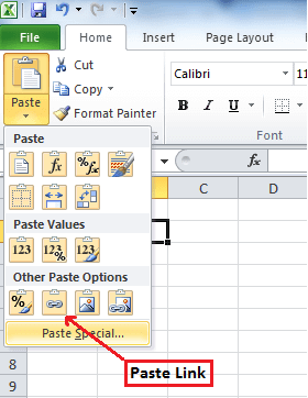
• Save all your work from the source worksheet before closing it

2) Manually enter the formula

• Open your destination worksheet, tap to the cell that is having a link formula and put an equal sign (=) across it
• Now go to the source sheet and tap to the cell which is having data. press Enter from your keyboard and save your tasks.

Note- Always remember one thing that the format of the source worksheet and the destination worksheet both are the same.

Method #2: Update Excel Spreadsheet With Data From Another Spreadsheet

To update Excel spreadsheets with data from another spreadsheet, just follow the points given below which will be applicable for the Excel version 2019, 2016, 2013, 2010, 2007.

• At first, go to the Data menu
• Select Refresh All option

• Here you have to see that when or how the connection is refreshed
• Now click on any cell that contains the connected data
• Again in the Data menu, click on the arrow which is next to Refresh All option and select Connection Properties

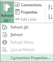
• After that in the Usage menu, set the options that you want to change
• On the Usage tab, set any options you want to change.

Note – If the size of the Excel data workbook is large, then I will recommend checking the Enable background refresh menu on a regular basis.

Method #3: How To Copy Data From One Cell To Another In Excel Automatically

To copy data from one cell to another in Excel, just go through the following points given below:

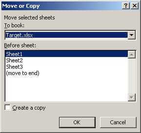
• First, open the source worksheet and the destination worksheet.
• In the source worksheet, navigate to the sheet that you want to move or copy
• Now, click on the Home menu and choose the Format option
• Then, select the Move Or Copy Sheet from the Organize Sheets part
• After that, again in the Home menu choose the Format option in the cells group
• Here in the Move Or Copy dialog option, select the target sheet and Excel will only display the open worksheets in the list

• Else, if you want to copy the worksheet instead of moving, then kindly make a copy of the Excel workbook before

• Lastly, select the OK button to copy or move the targeted Excel spreadsheet.

Method #4: How To Copy Data From One Sheet To Another In Excel Using Formula

You can copy data from one sheet to another in Excel using formula. Here are the steps to be followed:

• For copy and paste the Excel cell in the present Excel worksheet, as for example; copy cell A1 to D5, you can just select the destination cell D5, then enter =A1 and press the Enter key to get the A1 value.
• For copying and pasting cells from one worksheet to another worksheet such as copy cell A1 of Sheet1 to D5 of Sheet2, please select the cell D5 in Sheet2, then enter =Sheet1!A1 and press the Enter key to obtain the value.

Method #5: Copy Data From One Excel Sheet To Another Using Macros

With the help of macros, you can copy data from one worksheet to another but before this here are some important tips that you must take care of:

• You should keep the file extension correctly in your Excel workbook.
• It’s not necessary that your spreadsheet should be macro enable for doing the task.
• The code that you choose can also be stored in a different worksheet.
• As the codes already specify the details, so there is no need to activate the Excel workbook or cells first.
• Thus, given below is the code for performing this task.

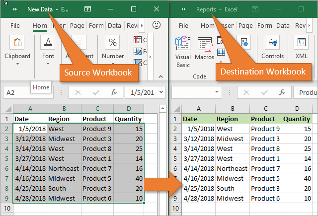
Sub OpenWorkbook()
‘Open a workbook
‘Open method requires full file path to be referenced.
Workbooks.Open “C:UsersusernameDocumentsNew Data.xlsx”

‘Open method has additional parameters
‘Workbooks.Open(FileName, UpdateLinks, ReadOnly, Format, Password, WriteResPassword, IgnoreReadOnlyRecommended, Origin, Delimiter, Editable, Notify, Converter, AddToMru, Local, CorruptLoad)

End Sub

Sub CloseWorkbook()
‘Close a workbook
Workbooks(“New Data.xlsx”).Close SaveChanges:=True
‘Close method has additional parameters
‘Workbooks.Close(SaveChanges, Filename, RouteWorkbook)

End Sub

Recommended Solution: MS Excel Repair & Recovery Tool

When you are performing your work in MS Excel and if by mistake or accidentally you do not save your workbook data or your worksheet gets deleted, then here we have a professional recovery tool for you, i.e. MS Excel Repair & Recovery Tool.

With the help of this tool, you can easily recover all lost data or corrupted Excel files also. This is a very useful software to get back all types of MS Excel files with ease.

* Free version of the product only previews recoverable data.

Steps to Utilize MS Excel Repair & Recovery Tool:

Conclusion:

Well, I tried my level best to provide the best possible ways to transfer data from one Excel worksheet to another automatically. So from now on, you don’t have to worry about how to copy data from one cell to another in Excel automatically.

I hope you are satisfied with the above methods provided to you about Excel worksheet update.

Thus, make proper use of them and in the future also if you want to know about this, you can take the help of the specified solutions.

In this tutorial, learn how to move data from one cell to another in Microsoft Excel Sheet. You can shift your data to other cell or column using a keyboard or mouse. There are various methods which are given below to change the place of data.

So, let’s start learning each method with the step-by-step- guide given below.

Move Data From One Cell to Another Using Mouse in Excel

To move data to other cells or columns using the only mouse, you have to follow the below steps. Use only your mouse to perform this task in a few easy steps.

Step 1 Enter Data in Excel

First of all, you have to enter any number of data in the Excel Sheet. Let’ take an example of data as given in the image below.

The example contains numbers in column B from cell B2 to B7. you have to now move this data to the cells of column D. Follow the next steps after entering the data.

Step 2 Select Data with Hover Over the Corner and Hold Mouse Left Button

Select your entire data using your mouse. After that, you have to hover over the corner of the selected data. You can hover to any corner position to the left, right, top and bottom.

Now, hold your mouse left button when you get the pointer sign as .

The above example showing the selected data. You can also find the pointer sign when you hover over the corner. Click the corner when you get the sign in the mouse pointer. Now, Keep your mouse hold for the next step.

Step 3 Drag-n-drop to the Cell to Move Data in Excel

You have to now drag your mouse to the required column cell. Drop the data when you reach the required cell to move to. It drops the whole data you have selected to move to the other cells.

The above example showing the image which you get when you drag your mouse.

Step 4 Final Moved Data

This is the final output contains the moved data to the cell of column D. The data copied from cell D2 to D7.

You can also move any of your data after selection using your mouse. If you want to move your data using a keyboard, you have to use the step-by-step process given below.

Shift One Cell Data to Another Using Only Keyboard in Excel Sheet

This is the method of only using the keyboard to change your data position. It’s the simple cut and paste method to shift data to other column cells.

Step 1 Put Your Data in Cell of Excel Sheet

Here, you also have to enter your data first in any cell of the Excel. Perhaps, you want to move the data already exist in the Excel sheet.

It depends upon you for which data you use. You can use any data to shift to other column cells. The above example showing the same data you have used in the above section.

Step 2 Select the Data Data Using Keyboard

Now, select your chosen data which you have to shift to the other cell. Use your keyboard left and right arrow key to move to the required data. Combination of shift and the arrow keys can be used to select the entire data.

The above image showing the selected data to shift to the other column cells.

Step 3 Press ‘CTRL + X’ to Cut Data

You have to cut the selected cell to shift to the other column cell. For this, press the keyboard key ‘CTRL + X’ to cut the data in Excel Sheet.

The above image showing the screen which you will get after pressing ‘CTRL + X’. This showing you are using the above data to cut in Excel Sheet.

Step 4 Go to Cell to Paste Data

After you perform the above step, you have to go to the cell where you want to place data. Press keyboard arrow keys to visit the required place for data.

The above example showing that you want to shift data to column D and start from cell D2.

Step 5 Press ‘CTRL + V’ to Paste and Move Data

The final step is to press the keyboard shortcut key ‘CTRL + V’. This is the key to paste the cut data to any required place of Excel Sheet.

The above image showing the shifted data to column D.

Change Data from One Column to Another in Excel

In addition to above all, you can also change or move one column data to another column. You have to first choose the data which you want to move. After that, follow the step-by-step guide given below with screenshots.

Step 1 Mouse Hover Over the Column Containing the Data

You have to first take your mouse to the column name which contains the required data. The pointer of the mouse changes to a down arrow like shape as given in the image.

The above image showing the data and the mouse pointer showing down arrow.

Step 2 Click Column Name to Select Data

Click the column name whose data you have to move. It selects all the cell of the clicked column name.

The above image showing the selected column containing the data to move.

Step 3 Mouse Right Click and Select ‘Cut’ Option

Now, you have to click the mouse right button to get various menu options. In the menu options, you have to select the ‘Cut’ option given on the menu.

You will get a highlighting column selection as showing in the image below.

Step 4 Click Column Name Where You Want to Shift Data

Click the column name to which you want to move the data. You will get a down arrow pointer for the mouse when you take your mouse to the column name.

The above example showing the select column where you have to place the data.

Step 5 Finally, press ‘CTRL + V’ to Paste Data

The final step is to paste the data using the keyboard shortcut ‘CTRL + V’. The below example image showing the pasted data to the new column.

You May Also Like to Read

• Copy Data In Alternate Rows Selected In Excel
• Quickly Select All Cells Of A Column In Excel
• Autofill Dates, Months And Current Time In Excel Sheet

Reference
MS Office Excel Doc to Move Cell and Cell Content

When working with data in Excel, you will often format data (such as color the cells or make them bold or give a border), to make these stand out.

And if you have to do this for many cells or range of cells, instead of doing it manually, you can do it once and then copy and paste the formatting.

In this tutorial, I will show you how to copy formatting in Excel. You can easily do it by using the Format painter option, using the Fill handle, or Paste special.

Copy the Formatting to a Single Cell

We’ll first see how to copy a formatting to a single cell in Excel. Let’s say that you have cell A2 formatted as an accounting number, with red background and white font color. 

In Cell C2 we have the plain number without any format.

1. Select a formatted cell that has the formatting that you want to copy (A2 in our example)
2. Click on Format Painter in the Home tab. This will change the cursor into a paintbrush with a plus icon

1. Click on a cell where you want to copy a format (C2)

Whenever you select a cell and choose Format Painter in the toolbar, the mouse cursor turns into a white cross with a brush.

This is how you know that the formatting is copied to the clipboard and you can paste it where you want.

Just the way we copied the formatting from one to another in the same sheet. you can also copy formatting to another sheet or another workbook. Simply select the cell from where you want to copy the formatting, enable format painter, select the sheet/workbook where you want to paste it, and select the cells in the destination sheet.

With Format Painter, you can easily copy the following formatting:

• Cell background-color
• Font size and color
• Font (including number format)
• Font characteristics (bold, italics, underline)
• Text alignment and orientation
• Cell borders (type, size, color)
• Custom Number Formatting
• Conditional Formatting

Personally. I find it a huge time saver to copy conditional formatting from one cell to another in the same sheet or other sheets. Excel is smart enough to adjust the rules in conditional formatting in case you’re using custom formulas.

Copy the Formatting to a Range of Cells

Just like you can copy the formatting from one cell to another cell, you can also copy it to a range of cells.

In this case, you need to select a range of cells on which you want to apply the format painter.

Suppose you have a dataset as shown below where you want to copy the formatting from cell A2 to the range of cells in C2:C7

1. Select a formatted cell (A2)
2. Click on Format Painter in the Home tab
3. Select a range of cells where you want to copy a format (C2:C7)

As a result, the format from A2 is copied to the selected range.

PRO TIP: When you click on the Format Paint icon, it allows you to format a cell or range of cells only once. Once you’re done, it’s disabled. So if you want to copy formatting to two ranges of cells, you will have to enable format painter twice. Alternatively, when you double-click on the Format Paint icon, it remains enabled and you can copy formatting to multiple cells or ranges.

Copy the Formatting Using Paste Special

When you copy and paste cells in Excel, you noticed that there are usually multiple paste options, such as: Paste text, Paste values, etc. 

One of these options is Paste formatting. 

This allows you to copy only the formatting from cells to cells.

1. Select and right-click a cell from which you want to copy the formatting (A2)
2. Click Copy (or use the keyboard shortcut CTRL+C).

1. Select a range of cells to which you want to copy the formatting (C2:C7);
2. Right-click anywhere in the selected range;
3. Click the arrow next to Paste Special;
4. Choose the icon for formatting.

The result is the same as using the Format painter.

You can also notice that all formatting that you copied by Format painter is also copied using the Paste special option.

Just like format painter, you can also use the Paste Special technique to paste formatting on the cells or range of cells in the same sheet or other sheet/workbook.

Pro Tip: If you have to copy the formatting from a cell to multiple cells that are scattered through the worksheet, you can use the paste special technique to copy formatting to one cell, and then repeat the process by using the F4 key. So copy the formatting once, then select another cell and press F4, and it will repeat your last action (which was to paste the formatting).

Also read: How to Copy and Paste in Excel Without Changing the Format?

Copy the Formatting Using the Fill Handle

As you probably already know, the fill handle is the little black cross that appears when you position a cursor in the right bottom corner of the cell (as shown below).

This cursor allows you to copy a cell (or range of cells) down the rows.

Apart from copying the cell values, the fill handle also allows you to copy the formatting.

Let’s say that you have a list of numbers in column A, where the first value in the list (A2) is formatted, while other values (A3:A7) are not formatted at all.

What I want is to copy the formatting from cell A2 to all the cells below it.

Below are the steps to do this:

1. Position the cursor in the right bottom corner of a cell from which you want to copy the formatting (A2) until the black cross (fill handle) appears;

1. Drag the fill handle down to the end of the range which we want to format (A7). If you want to copy the cell to the end of the range (until the first blank cell in the range), just double-click the fill handle.

1. When you drop the cursor, by default both value and formatting will be copied to the range. Now, you need to click on the AutoFill Options icon next to the end of the range and choose Fill Formatting Only.

Now, you can see that values are not changed, while the formatting is copied to the whole range.

While I have shown how to use the Fill Handle to copy formatting for one column only, you can use it the same way for the data in a row of data that spans across multiple rows and columns.

One drawback of using the fill handle is that your data needs to be in the same column or row where you have the cell from which you are copying the formatting.  This also means that you cannot use this method to copy the formatting to cells or range of cells that are in another sheet or workbook.

So these are some of the methods you can use to copy formatting from one cell to another cell or range of cells in Excel.

I hope you found this tutorial useful!

Other Excel tutorials you may also like:

• Using Conditional Formatting with OR Criteria in Excel
• How to Format Phone Numbers in Excel
• How to Highlight Every Other Row in Excel (Conditional Formatting & VBA)
• How to Copy Multiple Sheets to a New Workbook in Excel
• How to Create Barcodes in Excel
• How to Autofill Dates in Excel (Autofill Months/Years)
• How to Bold Text using VBA in Excel
• Shortcut to Paste without Formatting in Excel
• How to Change Theme Colors in Excel?
• How to Remove Conditional Formatting in Excel? (5 Easy Ways)
• How to Remove Table Formatting in Excel?
• Copy and Paste shortcuts in Excel