Copy formula in cell excel - Word и Excel - помощь в работе с программами

It’s important to be aware of the possibilities for how a relative cell reference might change when you move or copy a formula.

Moving a formula: When you move a formula, the cell references within the formula do not change no matter what type of cell reference that you use.
Copying a formula: When you copy a formula, relative cell references will change.

Move a formula

Select the cell that contains the formula that you want to move.
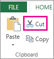
In the Clipboard group of the Home tab, click Cut.

You can also move formulas by dragging the border of the selected cell to the upper-left cell of the paste area. This will replace any existing data.
Do one of the following:
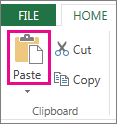
- To paste the formula and any formatting: In the Clipboard group of the Home tab, click Paste.
- To paste the formula only: In the Clipboard group of the Home tab, click Paste, click Paste Special, and then click Formulas.

Copy a formula

Select the cell containing the formula that you want to copy.
In the Clipboard group of the Home tab, click Copy.
Do one of the following:
- To paste the formula and any formatting, in the Clipboard group of the Home tab, click Paste.
- To paste the formula only, iIn the Clipboard group of the Home tab, click Paste, click Paste Special, and then click Formulas.
  
  Note: You can paste only the formula results. In the Clipboard group of the Home tab, click Paste, click Paste Special, and then click Values.
Verify that the cell references in the formula produce the result that you want. If necessary, switch the type of reference by doing the following:
1. Select the cell that contains the formula.
2. In the formula bar , select the reference that you want to change.
3. Press F4 to switch between the combinations.
  
  The table summarizes how a reference type will updates if a formula containing the reference is copied two cells down and two cells to the right.

For a formula being copied:	If the reference is:	It changes to:
	$A$1 (absolute column and absolute row)	$A$1
	A$1 (relative column and absolute row)	C$1
	$A1 (absolute column and relative row)	$A3
	A1 (relative column and relative row)	C3

Note: You can also copy formulas into adjacent cells by using the fill handle . After verifying that the cell references in the formula produce the result that you want in step 4, select the cell that contains the copied formula, and then drag the fill handle over the range that you want to fill.

Moving formulas is very much like moving data in cells. The one thing to watch for is that the cell references used in the formula are still what you want after you move.

Select the cell that contains the formula you want to move.
Click Home > Cut (or press Ctrl + X).
Select the cell you want the formula to be in, and then click Paste (or press Ctrl + V).
Verify that the cell references are still what you want.

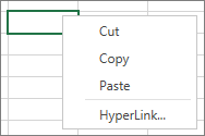
Tip: You can also right-click the cells to cut and paste the formula.

Источник

— By
Sumit Bansal

Watch Video – Copy and Paste Formulas in Excel without Changing Cell References

When you copy and paste formulas in Excel, it automatically adjusts the cell references.

For example, suppose I have the formula =A1+A2 in cell B1. When I copy the cell B1 and paste it in B2, the formula automatically becomes =A2+A3.

This happens as Excel automatically adjusts the references to make sure the rows and columns now refer to the adjusted rows and columns.

Note: This adjustment happens when you’re using relative references or mixed references. In the case of absolute references, the exact formula gets copied.

Copy and Paste Formulas in Excel without Changing Cell References

When using relative/mixed references in your formulas, you may – sometimes – want to copy and paste formulas in Excel without changing the cell references.

Simply put, you want to copy the exact formula from one set of cells to another.

In this tutorial, I will show you how you can do this using various ways:

Manually Copy Pasting formulas.
Using ‘Find and Replace’ technique.
Using the Notepad.

Manually Copy Paste the Exact Formula

If you only have a handful of formulas that you want to copy and paste without changing the cell references, doing it manually would be more efficient.

To copy paste formulas manually:

Select the cell from which you want to copy the formula.
Go to the formula bar and copy the formula (or press F2 to get into the edit mode and then copy the formula).
Select the destination cell and paste the formula.

Note that this method works only when you have a few cells from which you want to copy formulas.

If you have a lot, use the find and replace technique shown below.

Using Find and Replace

Here are the steps to copy formulas without changing the cell references:

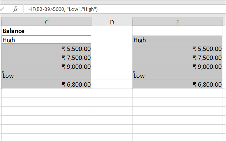
This will convert the text back into the formula and you will get the result.

Note: If you use the # character as a part of your formula, you can use any other character in Replace with (such as ‘ZZZ’ or ‘ABC’).

Using Notepad to Copy Paste Formulas

If you have a range of cells where you have the formulas that you want to copy, you can use a Notepad to quickly copy and paste the formulas.

Here are the steps to copy formulas without changing the cell references:

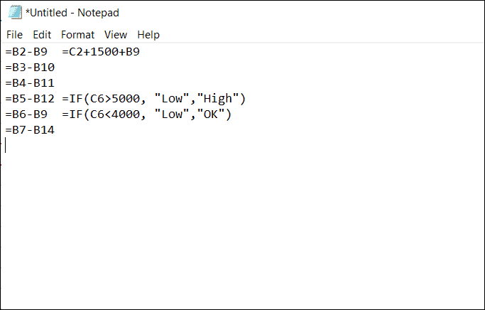
Go to Formulas –> Show Formulas. This will show all the formulas in the worksheet.
Copy the cells that have the formulas that you want to copy.
Open a notepad and paste the cell contents in the notepad.
Copy the content on the notepad and paste in the cells where you want the exact formulas copied.
Again go to Formulas –> Show formulas.

Note: Instead of Formulas –> Show formulas, you can also use the keyboard shortcut Control + ` (this is the same key that has the tilde sign).

You May Also Like the Following Tutorials:

How to Convert Formulas to Values in Excel.
Show Formulas in Excel Instead of the Values.
How to Lock Formulas in Excel.
Understanding Absolute, Relative, and Mixed Cell References in Excel.
How to reference another sheet in Excel.
How to Remove Cell Formatting in Excel
How to Copy Excel Table to Word
How to Copy and Paste Column in Excel?
How to Multiply a Column by a Number in Excel

Get 51 Excel Tips Ebook to skyrocket your productivity and get work done faster

31 thoughts on “How to Copy and Paste Formulas in Excel without Changing Cell References”

Thank you for your help.
“Using Find and Replace” is very good option. it really works.
Thank you very much
BROOOOOO! This was so smart and easy. Thanks my friend!
Excellent. That has made my work today so much easier!!
Thanks you so much! This Helped me a lot!!
Great! Thanks for the teaching! Loving the Notepad method
Amazing….such a nice n easy way to do it with replace..thanks a lot
Thanks alot. really helpful
Nice. Very well explained, thank you.
OH. MY. GOSH. I’m 10 hours of copying and pasting formulas but this has saved me at least a few more and countless future hours! Replacing = with #, pasting, then replacing # with =. It’s so simple… why didn’t I think of it. 🙂 Thank you!
Thanks a lot Simple & Eazy
# is best and easiest solution, thanks a lot!!! very clever!
thanks a lot
This saved me tonnes of work. Thanks so much!
For a copying and pasting a large array of formulas comprising both relative and absolute references to different cells, sheets and workbooks, the ‘find and replace’ has proven to be convoluted, time consuming and problematic. One has to ‘cherry pick’ through the array to ensure which of one’s relative cell references are not to be changed.
I migrated to excel from lotus-123; as a comparison using ‘123’ back then, one would simply ‘highlight rows (or columns)’, ‘copy’, ‘insert’ equal rows (or columns), then ‘paste’ – quick and most importantly no cherry picking errors.
Excel’s ‘insert copied cells’ command hides the ‘insert row or column’ command, therefore one cannot emulate the ‘123’ way. Even if one tries the ‘insert sheet rows (or columns)’ command then attempt to paste directly from ‘clipboard’, only text and not formulas are pasted.
amazing!
thanks
saved me 20 min. of work…
THIS IS AWESOME! – THE # = TRICK. GENIUS!
THANK U VERY MUCH!
- Agree! This is so simple, but very helpful. Thanks!
I have a cell reference issue I hope someone can help me with. I have a cell outside of a range that I always want to refer to a specific cell inside of the range, even when cells are inserted or deleted from the range. For example, cell A10 refers to C10 in the range B1:D200. If someone inserts cells B7:D13, I still want A10 to refer to C10, not C17. I think I need a helper column that has the text “C10” in cell E10. What is the Function that gets A10 to use the static text in E10 to refer to cell C10?
- You can use the INDIRECT function. This should work =INDIRECT(“C10”). If you have text C10 in cell E10, just use =INDIRECT(E10)
  - Thanks. That is the Function I was looking for, but could not remember.
  - Even though INDIRECT is less complicated, can you tell me why CELL(“contents”,ADDRESS(10,3)) didn’t work?
    - Jim,
      although these are functions I’ve never had cause to use, I think this might be because the $C$10 from the ADDRESS function is seen as text, not a cell reference
      CELL(“contents”,”$C$10″) certainly does not work
      regards,
      t’other jim
  - although INDIRECT is the way to go with this, you could also use OFFSET:
    =OFFSET(A10,,2) should work
    both are volatile formulae (will recalculate on every worksheet change), which you might be able to avoid by using =INDEX(C:C,10) which would only fail your requirements if a whole column were inserted or deleted somewhere between A:A and C:C
    - taking this a step further, =INDEX(1:1048576,10,3) will always refer to C10 – but it’s very clumsy-looking
- I’ve made a step in the right direction. ADDRESS(10,3) results in $C$10 and it does not change when cell C10 is moved. CELL(“contents”,$C$10) gives me the proper result. However, CELL(“contents”,ADDRESS(10,3)) is not even accepted. What is wrong with the nested formula?
  - you should use “=CELL(“contents”, INDIRECT(ADDRESS(10,3,1,1,”Sheet1″),1))” as there are certain arguments to ADDRESS function which ADDRESS(10,3) is not capturing and those arguments are not optional.
I think Bansal’s point was that sometimes you can have a range of dynamic formulae that you want to replicate elsewhere
I’ve had this situation occur before but I never thought of using the Notepad method – thanks for that, another weapon in my arsenal
Absolute cell reference is the best. i.e. =A$1$ + B$1$ this cell is locked in that way.
I use absolute/Dynamic references for doing this
- I love method 3. Thanks you.

Comments are closed.

Источник

Download Article

Using Find and Replace

Filling a Column or Row

Pasting a Formula into Multiple Cells

Using Relative and Absolute Cell References

Video

Tips

Warnings

Excel makes it easy to copy your formula across an entire row or column, but you don’t always get the results you want. If you end up with unexpected results, or those awful #REF and /DIV0 errors, it can be extremely frustrating. But don’t worry—you won’t need to edit your 5,000 line spreadsheet cell-by-cell. This wikiHow teaches you easy ways to copy formulas to other cells.

Open your workbook in Excel. Sometimes, you have a large spreadsheet full of formulas, and you want to copy them exactly. Changing everything to absolute cell references would be tedious, especially if you just want to change them back again afterward. Use this method to quickly move formulas with relative cell references elsewhere without changing the references.^[1] In our example spreadsheet, we want to copy the formulas from column C to column D without changing anything.

Example Spreadsheet

	Column A	Column B	Column C
row 1	944	Frogs	=A1/2
row 2	636	Toads	=A2/2
row 3	712	Newts	=A3/2
row 4	690	Snakes	=A4/2

If you’re just trying to copy the formula in a single cell, skip to the last step («Try alternate methods») in this section.

2

Press Ctrl+H to open the Find window. The shortcut is the same on Windows and macOS.

Advertisement

Find and replace «=» with another character. Type «=» into the «Find what» field, and then type a different character into the «Replace with» box. Click Replace All to turn all formulas (which always begin with an equal’s sign) into text strings beginning with some other character. Always use a character that you have not used in your spreadsheet. For example, replace it with # or &, or a longer string of characters, such as ##&.

Example Spreadsheet

	Column A	Column B	Column C
row 1	944	Frogs	##&A1/2
row 2	636	Toads	##&A2/2
row 3	712	Newts	##&A3/2
row 4	690	Snakes	##&A4/2

Do not use the characters * or ?, since these will make later steps more difficult.

Copy and paste the cells. Highlight the cells you want to copy, and then press Ctrl + C (PC) or Cmd + C (Mac) to copy them. Then, select the cells you want to paste into, and press Ctrl + V (PC) or Cmd + V (Mac) to paste. Since they are no longer interpreted as formulas, they will be copied exactly.

Example Spreadsheet

	Column A	Column B	Column C	Column D
row 1	944	Frogs	##&A1/2	##&A1/2
row 2	636	Toads	##&A2/2	##&A2/2
row 3	712	Newts	##&A3/2	##&A3/2
row 4	690	Snakes	##&A4/2	##&A4/2

Use Find & Replace again to reverse the change. Now that you have the formulas where you want them, use «Replace All» again to reverse your change. In our example, we’ll look for the character string «##&» and replace it with «=» again, so those cells become formulas once again. You can now continue editing your spreadsheet as usual:

Example Spreadsheet

	Column A	Column B	Column C	Column D
row 1	944	Frogs	=A1/2	=A1/2
row 2	636	Toads	=A2/2	=A2/2
row 3	712	Newts	=A3/2	=A3/2
row 4	690	Snakes	=A4/2	=A4/2

6
Try alternate methods. If the method described above doesn’t work for some reason, or if you are worried about accidentally changing other cell contents with the «Replace all» option, there are a couple other things you can try:
- To copy a single cell’s formula without changing references, select the cell, then copy the formula shown in the formula bar near the top of the window (not in the cell itself). Press Esc to close the formula bar, then paste the formula wherever you need it.
- Press Ctrl and ` (usually on the same key as ~) to put the spreadsheet in formula view mode. Copy the formulas and paste them into a text editor such as Notepad or TextEdit. Copy them again, then paste them back into the spreadsheet at the desired location. Then, press Ctrl and ` again to switch back to regular viewing mode.

Type a formula into a blank cell. Excel makes it easy to propagate a formula down a column or across a row by «filling» the cells. As with any formula, start with an = sign, then use whichever functions or arithmetic you’d like. We’ll use a simple example spreadsheet, and add column A and column B together. Press Enter or Return to calculate the formula.

Example Spreadsheet

	Column A	Column B	Column C
row 1	10	9	19
row 2	20	8
row 3	30	7
row 4	40	6

2

Click the lower right corner of the cell with the formula you want to copy. The cursor will become a bold + sign.

Click and drag the cursor across the column or row you’re copying to. The formula you entered will automatically be entered into the cells you’ve highlighted. Relative cell references will automatically update to refer to the cell in the same relative position rather than stay exactly the same. Here’s our example spreadsheet, showing the formulas used and the results displayed:

Example Spreadsheet

	Column A	Column B	Column C
row 1	10	9	=A1+B1
row 2	20	8	=A2+B2
row 3	30	7	=A3+B3
row 4	40	6	=A4+B4

Example Spreadsheet

	Column A	Column B	Column C
row 1	10	9	19
row 2	20	8	28
row 3	30	7	37
row 4	40	6	46

You can also double-click the plus sign to fill the entire column instead of dragging. Excel will stop filling out the column if it sees an empty cell. If the reference data contains a gap, you will have to repeat this step to fill out the column below the gap.
Another way to fill the entire column with the same formula is to select the cells directly below the one containing the formula and then press Ctrl + D.^[2]

Type the formula into one cell. As with any formula, start with an = sign, then use whichever functions or arithmetic you’d like. We’ll use a simple example spreadsheet, and add column A and column B together. When you press Enter or Return, the formula will calculate.

Example Spreadsheet

	Column A	Column B	Column C
row 1	10	9	19
row 2	20	8
row 3	30	7
row 4	40	6

2

Select the cell and press Ctrl+C (PC) or ⌘ Command+C (Mac). This copies the formula to your clipboard.
3

Select the cells you want to copy the formula to. Click on one and drag up or down using your mouse or the arrow keys. Unlike with the column or row fill method, the cells you are copying the formula to do not need to be adjacent to the cell you are copying from. You can hold down the Control key while selecting to copy non-adjacent cells and ranges.
4

Press Ctrl+V (PC) or ⌘ Command+V (Mac) to paste. The formulas now appear in the selected cells.

1

Use a relative cell reference in a formula. In an Excel formula, a «cell reference» is the address a cell. You can type these in manually, or click on the cell you wish to use while you are entering a formula. For example, the following spreadsheet has a formula that references cell A2:

Relative References

Column A Column B Column C

row 2
50

7

=A2*2

row 3
100

row 4
200

row 5
400
2
Understand why they’re called relative references. In an Excel formula, a relative reference uses the relative position of a cell address. In our example, C2 has the formula “=A2”, which is a relative reference to the value two cells to the left. If you copy the formula into C4, then it will still refer to two cells to the left, now showing “=A4”.

Relative References

Column A Column B Column C

row 2
50

7

=A2*2

row 3
100

row 4
200

=A4*2

row 5
400
- This works for cells outside of the same row and column as well. If you copied the same formula from cell C1 into cell D6 (not shown), Excel would change the reference «A2» to a cell one column to the right (C→D) and 5 rows below (2→7), or «B7».
3
Use an absolute reference instead. Let’s say you don’t want Excel to automatically change your formula. Instead of using a relative cell reference, you can make it absolute by adding a $ symbol in front of the column or row that you want to keep the same, no matter where you copy the formula too.^[3] Here are a few example spreadsheets, showing the original formula in larger, bold text, and the result when you copy-paste it to other cells:
- Relative Column, Absolute Row (B$3): The formula has an absolute reference to row 3, so it always refers to row 3:
  
  Column A Column B Column C
  
  row 1
  50
  
  7
  
  =B$3
  
  row 2
  100
  
  =A$3
  
  =B$3
  
  row 3
  200
  
  =A$3
  
  =B$3
  
  row 4
  400
  
  =A$3
  
  =B$3
- Absolute Column, Relative Row ($B1): The formula has an absolute reference to column B, so it always refers to column B.
  
  Column A Column B Column C
  
  row 1
  50
  
  7
  
  =$B1
  
  row 2
  100
  
  =$B2
  
  =$B2
  
  row 3
  200
  
  =$B3
  
  =$B3
  
  row 4
  400
  
  =$B4
  
  =$B4
- Absolute Column & Row ($B$1): The formula has an absolute reference to column B of row 1, so it always refers to column B of row 1.
  
  Column A Column B Column C
  
  row 1
  50
  
  7
  
  =$B$1
  
  row 2
  100
  
  =$B$1
  
  =$B$1
  
  row 3
  200
  
  =$B$1
  
  =$B$1
  
  row 4
  400
  
  =$B$1
  
  =$B$1
4

Use the F4 key to switch between absolute and relative. Highlight a cell reference in a formula by clicking it and press F4 to automatically add or remove $ symbols. Keep pressing F4 until the absolute or relative references you’d like are selected, then press Enter or Return.

	Column A	Column B	Column C
row 2	50	7	=A2*2
row 3	100
row 4	200
row 5	400

	Column A	Column B	Column C
row 2	50	7	=A2*2
row 3	100
row 4	200		=A4*2
row 5	400

	Column A	Column B	Column C
row 1	50	7	=B$3
row 2	100	=A$3	=B$3
row 3	200	=A$3	=B$3
row 4	400	=A$3	=B$3

	Column A	Column B	Column C
row 1	50	7	=$B1
row 2	100	=$B2	=$B2
row 3	200	=$B3	=$B3
row 4	400	=$B4	=$B4

	Column A	Column B	Column C
row 1	50	7	=$B$1
row 2	100	=$B$1	=$B$1
row 3	200	=$B$1	=$B$1
row 4	400	=$B$1	=$B$1

Add New Question

Question

When I try to pull down formula, it stays the same and does not change with row, what can I do?

Go to Formulas, Calculation Options, and change them from Manual to Automatic.
Question

When I click and drag, it copies the format also. I don’t want to copy the format, just the formula?

Krisztian Toth

Community Answer

Right after the drag there should be an icon in the lower right corner of the highlighted area. Hover over that and select from the various fill options, among which you can find an option to fill without format.
Question

How do I copy a date formula I have created (that includes the week day as well as date) so that it runs in sequence?

Krisztian Toth

Community Answer

Double click into the cell, copy your formula, double click into the destination cell, then press Ctrl+V or Command+V.

Ask a Question

200 characters left

Include your email address to get a message when this question is answered.

Submit

If you copy a formula to a new cell and see a green triangle, Excel has detected a possible error. Examine the formula carefully to see if anything went wrong.^[4]
If you accidentally did replace the = character with ? or * in the «copying a formula exactly» method, searching for «?» or «*» will not give you the results you expect. Correct this by searching for «~?» or for «~*» instead.^[5]
Select a cell and press Ctrl‘ (apostrophe) to fill it with the formula directly above it.

Thanks for submitting a tip for review!

Different versions of Excel may not show exactly the same screenshots in the same ways as are displayed here.

References

About This Article

Article SummaryX

To copy a formula into multiple adjoining cells in Microsoft Excel, type the formula into a cell, and then press Enter or Return to calculate it. Hover your mouse cursor over the bottom-right corner of the cell so the cursor turns to a crosshair, then drag the crosshair down to copy the formula to other cells in the column. If you’d rather copy the formula to cells in a row, drag the crosshair left or right.
To copy a formula to cells that aren’t touching the formula cell, click the cell once to select it, and then press Control + C (on a PC) or Command + C (on a Mac) to copy the formula. Now, select the cell or cells you want to copy the formula to, then press Control + V (on a PC) or Command + V (on a Mac) to paste it into the selected cells.

Did this summary help you?

Thanks to all authors for creating a page that has been read 513,635 times.

Is this article up to date?

Источник

Copying formulas is one of the most common and easiest tasks that you do in a typical spreadsheet that relies mainly on formulas. Rather than typing the same formula over and over again in Excel, you can just easily copy and paste a formula from one cell to multiple cells.

After writing a formula in Excel, you can use the copy and paste commands to multiple cells, multiple non-adjacent cells, or entire columns. If you don’t do it right, you’ll end up with that awful # REF and /DIV0 errors. In this article, we’ll show you the different methods you can use to copy formulas in Excel.

How to Copy and Paste Formulas in Excel

Microsoft Excel provides various ways to copy formulas with relative cell references, absolute cell references, or mixed references.

Copy formula from one cell to another
Copy formula one cell to multiple cells
Copying formula to the entire column
Copying formula without formatting
Copy formulas to non-adjacent cells
Copy formulas without changing cell references

How to Copy a Formula from One Cell to Another in Excel

Sometimes you may want to copy a formula from one cell to another in excel to avoid retyping the entire formula all over again and save some time while doing that.

Let’s say we have this table:

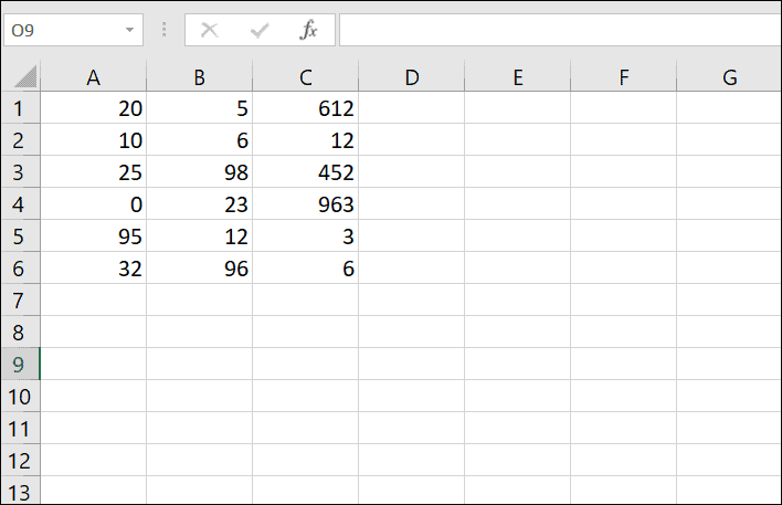
There are few methods to copy formula from one cell to another.

First, select the cell with the formula and right-click, and in the context menu, select ‘Copy’ to copy the formula. Or you can use the ‘Copy’ option in the ‘Clipboard’ section of the ‘Home’ tab.

But you also copy formulas by simply pressing the keyboard shortcut Ctrl + C. This is a more efficient and time-saving method.

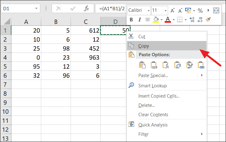
Then we go to the cell we want to paste it press the shortcut Ctrl + V to paste the formula. Or right-click on the cell you want to paste and click the options under ‘Paste Options’: either simple ‘Paste (P)’ option or paste as ‘Formula (F)’ option.

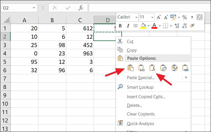
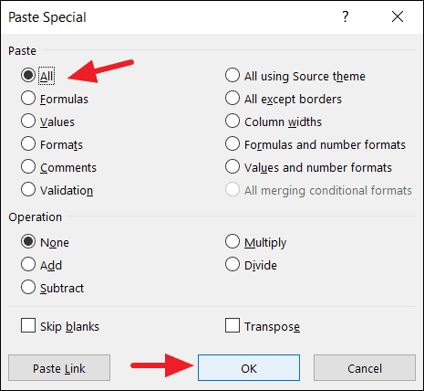
Alternatively, you can also click on ‘Paste Special’ below the six paste icons to open the ‘Paste Special’ dialog box. Here, you have several options including the six paste options from the context menu. Select ‘All’ or ‘Formulas’ under the Paste section and click ‘OK’.

Now the cell with pasted formula should have the same formulas (as the one in copied cell) but with the different cell references. The cell address is self adjusted by the excel to match row number of the pasted cell.

Copy Formula from One Cell to Multiple Cells

The same paste operation works just the same if we select multiple cells or a range of cells.

Select the cell with the formula and press Ctrl + C to copy the formula. Then, select all the cells where you want to paste the formula and press Ctrl + V to paste the formula or use one of the above paste methods to paste the formula (like we did for the single cell).

Copy Formula to an Entire Column or Row

In Excel, you can quickly copy a formula to an entire column or a row.

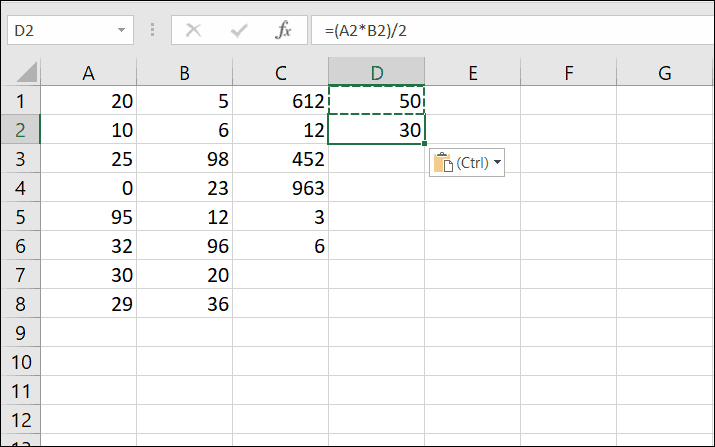
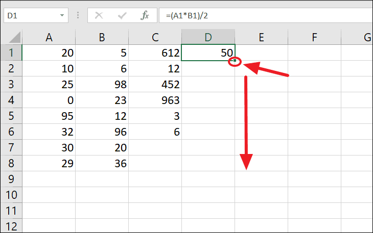
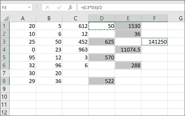
To copy a formula to a column or a row, first, enter a formula in a cell. Then, select the formula cell (D1), and hover your cursor over a small green square at the lower right corner of the cell. As you hover, the cursor will change to a black plus sign (+), which is called the Fill Handle. Click and hold that fill handle, and drag it in any direction you want (column or row) over the cells to copy the formula.

When you copy a formula to a range of cells, cell references of the formula will automatically adjust based on the relative location of rows and columns and the formula will perform calculations based on the values in those cell references (See below).

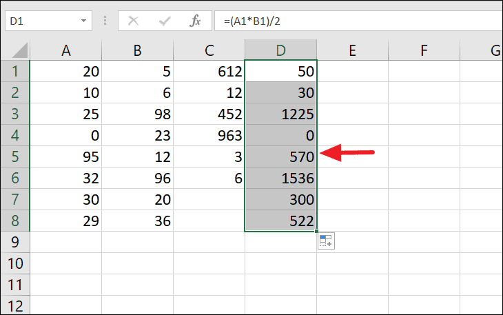
In the above example, when formula in D1 (=A1*B1)/2) copied to cell D2, the relative reference changes bases on it’s location (=A2*B2)/2) and so on.

In the same way, you can drag the formula into adjacent cells to the left, to the right, or upwards.

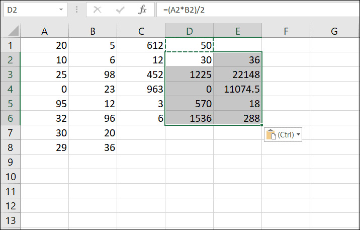
Another way to copy the formula to an entire column is by double-clicking the fill handle instead of dragging it. When you double-click the fill handle, it immediately applies the formula as far as there is any data to the adjacent cell.

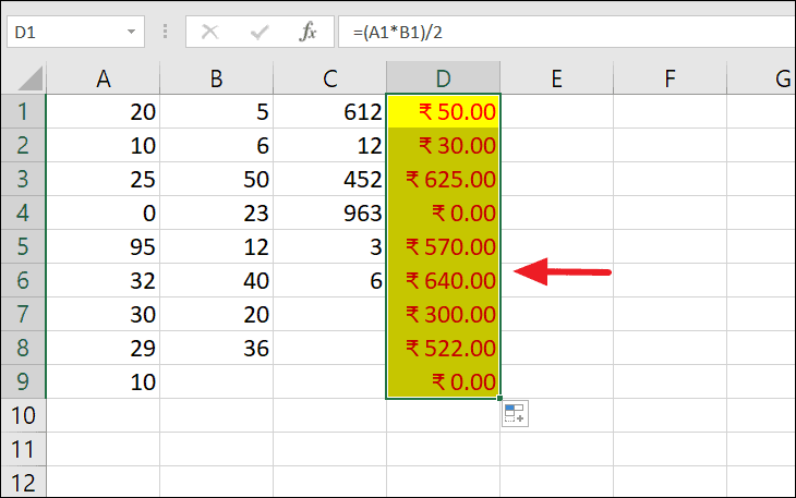
Copy a Formula to a Range Without Copying Formatting

When you copy a formula to a range of cells with the fill handle, it copies the source cell’s formatting too, such as font color or background color, currency, percentage, time, etc (as shown below).

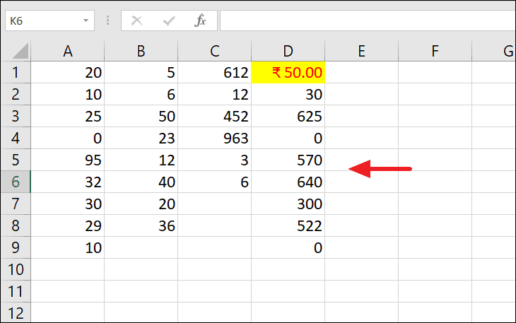
To prevent copying the cell formatting, drag the fill handle and click the ‘Auto Fill Options’ at the lower right-hand corner of the last cell. Then, in the drop-down menu, select ‘Fill Without Formatting’.

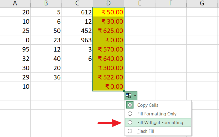
The result:

Copy an Excel Formula with Only Number Formatting

If you want to copy the formula with only the formula and the formatting such as percentage format, decimal points, etc.

Copy the formula and select all the cells to which you want to copy the formula. On the ‘Home’ tab, click the arrow below the ‘Paste’ button on the ribbon. Then, click the ‘Formulas & Number Formatting’ icon (the icon with % fx) from the drop-down to paste only the formula and the number formatting.

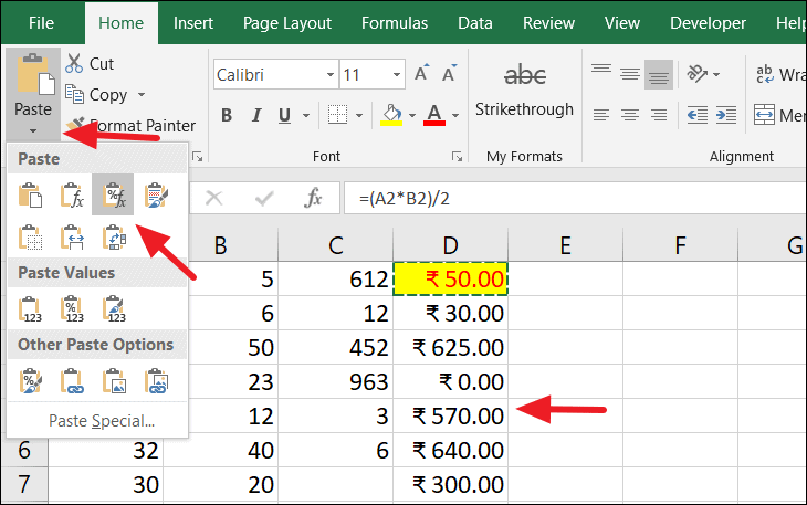
This option only copies formula and number formatting but ignores all other cell formattings like background color, font color, etc.

Copy a Formula to Non-Adjacent/Non-Contiguous Cells

If you want to copy a formula to non-adjacent cells or non-adjacent ranges, you can do that with the help of Ctrl key.

Select the cell with the formula and press Ctrl + C to copy it. Then, select non-adjacent cells/ranges while pressing and holding the Ctrl key. Then, press Ctrl + V to paste the formula and hit Enter to complete.

Copying Formulas Without Changing Cell References in Excel

When a formula is copied to another cell, Excel automatically changes the cell references to match its new location. These cell references use the relative location of a cell address, hence they are called relative cell reference (without $). For example, if you have the formula ‘=A1*B1’ in cell C1, and you copy this formula to cell C2, the formula will change to ‘=A2*B2’. All the methods we discussed above use relative references.

When you copy a formula with relative cell references, it automatically changes references so that the formula refers to the corresponding rows and columns. If you use absolute references in a formula, then the same formula gets copied without changing the cell references.

When you put a dollar sign ($) in front of the column letter and row number of a cell (For example $A$1), it turns the cell into an absolute cell. Now no matter where you copy the formula that contains the absolute cell reference, the formula will never. But if you have relative or mixed cell reference in a formula, use any of these following methods to copy without changing cell references.

Copy Formula with Absolute Cell Reference Using Copy-Paste Method

Occasionally, you may need to copy/apply the exact formula down the column, without changing the cell references. If you want to copy or move an exact formula with absolute reference, then do this:

First, select the cell with the formula you want to copy. Then, click on the formula bar, select the formula using the mouse, and press Ctrl + C to copy it. If you want to move the formula, press Ctrl + X to cut it. Next, hit the Esc key to leave the formula bar.

Alternatively, select the cell with the formula and hit F2 key or double-click the cell. This will put the selected cell into edit mode. Then, select the formula in the cell and hit Ctrl + C to copy the formula in the cell as text.

Then, select the destination cell and press Ctrl + V to paste the formula.

Now the exact formula gets copied into the destination cell without any cell reference changes.

Copy Formulas with Absolute or Mixed Cell References

If you’d like to move or copy exact formulas without changing cell references, you should change cell relative references to absolute references. For example, adding ($) sign to relative cell reference (B1) makes it an absolute reference ($B$1), so it remains static no matter where the formula is copied or moved.

But sometimes, you may need to use mixed cell references ($B1 or B$1) by adding a dollar ($) sign in front of the column letter or the row number to lock either a row or a column in place.

Let us explain with an example. Suppose you have this table that calculates the monthly savings by subtracting rent (B9) from earnings (in column B) every month.

In the example below, the formula uses an absolute cell reference ($B$9) to lock the rent amount to cell B9, and a relative cell reference to cell B2 because it needs to be adjusted for each row to match each month. B9 is made absolute cell reference ($B$9) because you want to subtract the same rent amount from each month’s earnings.

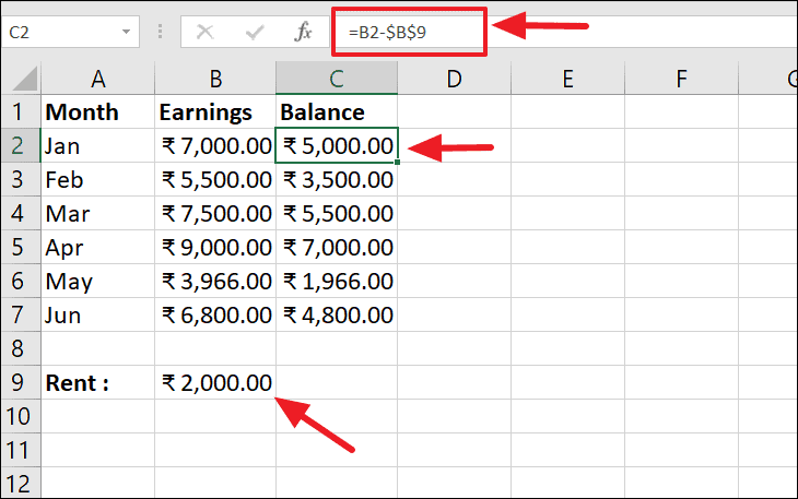
Let’s say you want to move the balances from column C to column E. If you copy the formula (by usual copy/paste method) from cell C2 (=B2-$B$9) will change to =D2-$B$9 when pasted in cell E2, making your calculations all wrong!

In that case, change the relative cell reference (B2) to a mixed cell reference ($B2) by adding the ‘$’ sign in front of the column letter of the formula entered in the cell C2.

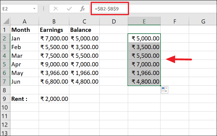
And now, if you copy or move the formula from cell C2 to E2, or any other cell, and apply formula down the column, the column reference will remain the same while the row number will be adjusted for each cell.

Copy Paste Excel Formulas Without Changing References Using Notepad

You can see every formula in your Excel spreadsheet by using Show Formula options. To do that go to the ‘Formulas’ tab and select ‘Show Formulas’.

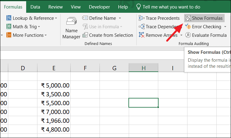
Alternatively, you can enter the formula view mode by pressing the Ctrl + ` shortcut, which displays every formula in your worksheet. You can find the grave accent key (`) at the top left corner of your keyboard on the row with the number keys (below the ESC key and before the number 1 key).

Select all the cells with the formulas you want to copy and press Ctrl + C to copy them, or Ctrl + X to cut them. Then open Notepad and press Ctrl + V to paste the formulas in the notepad.

Next, select the formula and copy(Ctrl + C) it from the notepad, and paste it(Ctrl + V) in the cell where you want the exact formula copied. You can copy and paste them one by one or all at once.

After pasting the formulas, turn off the formula view mode by pressing Ctrl + ` or again go to ‘Formulas’ –> ‘Show formulas’.

Copy the Exact Formulas Using Excel’s Find and Replace

If you want to copy a range of Exact formulas, you can also use Excel’s Find and Replace tool to do so.

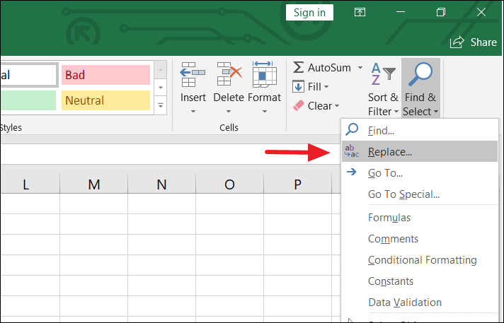
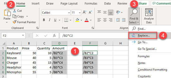
Select all the cells that have the formulas that you want to copy. Then go to the ‘Home’ tab, click ‘Find & Select’ on the Editing group, and select the ‘Replace’ option, Or simply press Ctrl + H to open the Find & Replace dialog box.

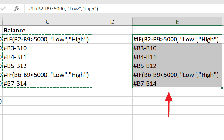
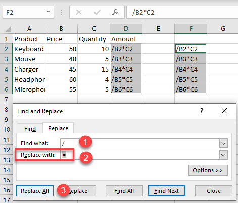
In the Find and Replace dialog box, enter the equal sign (=) in the ‘Find what’ field. In the ‘Replace with’ field, enter a symbol or character that is not already part of your formulas, like #, or , etc. Then, click the ‘Replace All’ button.

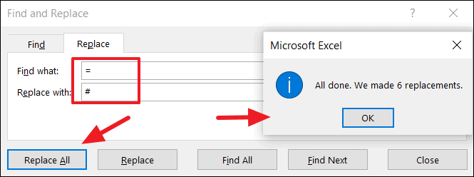
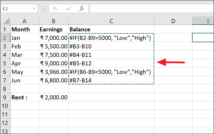
You’ll get a prompt message box saying ‘We made 6 replacements’ (because we selected 6 cells with formulas). Then click ‘OK’ and ‘Close’ to close both dialogs. Doing this replaces all equal to (=) signs with hash (#) signs, and turns formulas into text strings. Now the cell references of the formulas won’t be changed when copied.

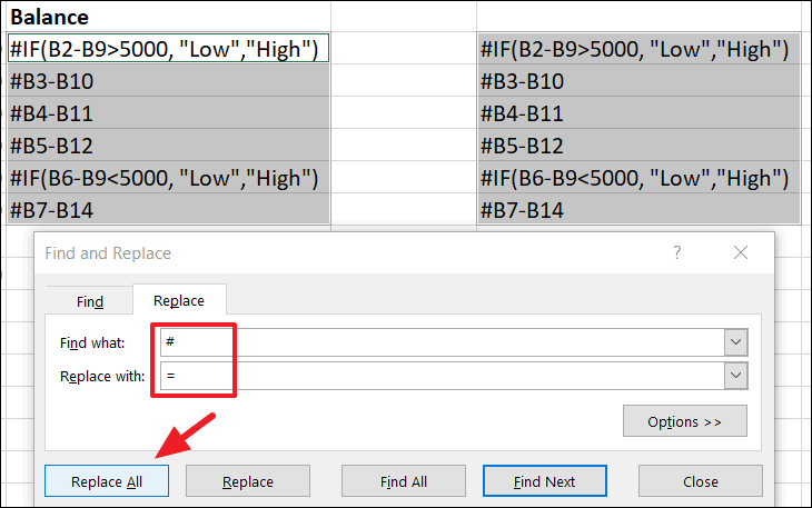
Now, you can select these cells, press Ctrl + C to copy them, and paste them into destination cells with Ctrl + V.

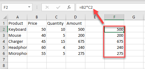
Finally, you need to change the (#) signs back to (=) signs. To do that, select both ranges (original and copied range) and press Ctrl + H to open the Find & Replace dialog box. This time, type the hash (#) sign in the ‘Find what’ field, and equal to (=) sign in the ‘Replace with’ field, and click the ‘Replace All’ button. Click ‘Close’ to close the dialog.

Now, the text strings are converted back to the formulas and you will get this result:

Done!

Источник

In this article we’ll learn how to copy formulas in Excel without changing the cell reference or in simple words we can say that how to copy exact formula from one cell to another cell.

There are two ways which you can follow to copy formulas from a range of cells without changing the Absolute reference or Relative reference in Microsoft Excel.

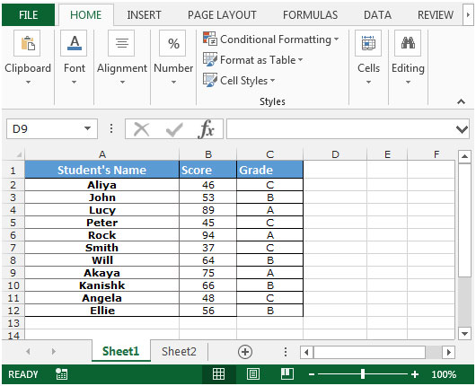
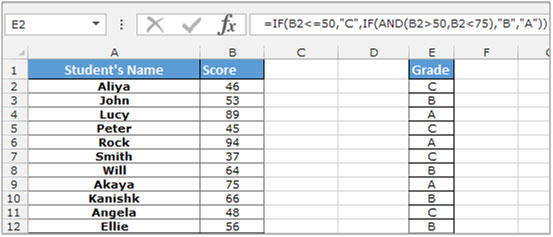
Let’s take an example to copy the formula from a range without changing the cell reference. We have a score card, in which column A contains Student’s name, column B contains scores and column C contains the formula for grades as per the criteria.

Now we need the grade to be copied to another location instead of column C, along with the formulae.

Follow the below given steps to copy the formula to another location: —

Select the range of cells containing the formulas and press “CTRL+H”.
In the Find what box, type the = sign.
In the Replace with box, type the # sign (to change the formulae to text).
Click Replace All, and then click on Close.
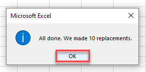
You will get a popup saying “All done. We made 22 replacements”.
Click on Ok.

Copy and paste these cells to a new location by pressing the keys “CTRL + C” to copy and then “CTRL+V” to paste it.
Select the new range containing the formulae and press Ctrl+H.
In the Find what box, type the # sign.
In the Replace with box, type the = sign (to change the text to formula).
Click on Replace All and then click on Close.
You will get a popup “All done. We made 22 replacements”.
Click on Ok.

You can then revert the column C to its original formulae instead of text, by replacing the “#” to “=” following the above steps.

Incase you want to move the formula to another location, you can follow the below given steps –

Select the range of cells containing the formulas and cut the formula by pressing the key “CTRL+X” on your keyboard.
Paste the range to the new location by pressing the key “CTRL+V”.

To remove the formula from data we can use the “Paste Special” option:-

Select the range E2:E12, copy by pressing the key “CTRL + C” on your keyboard.
Right click on the mouse and select “Paste Special”.
In the dialog box select values and click OK.
The formula will be replaced by its values.

If you liked our blogs, share it with your friends on Facebook. And also you can follow us on Twitter and Facebook.
We would love to hear from you, do let us know how we can improve, complement or innovate our work and make it better for you. Write us at info@exceltip.com

Источник

When you copy a formula, Excel automatically adjusts the cell references for each new cell the formula is copied to.

Copy 101

Simply use CTRL + c and CTRL + v to copy and paste a formula in Excel.

1. For example, to copy a formula, select cell A3 below and press CTRL + c.

2. To paste this formula, select cell B3 and press CTRL + v.

3. Click in the formula bar to clearly see that the formula references the values in column B.

Fill Handle

Use the fill handle in Excel to quickly copy a formula to other cells.

1. For example, select cell A3 below, click on the lower right corner of cell A3 (the fill handle) and drag it across to cell F3.

Result.

You can also use the fill handle to quickly copy a formula down a column.

2. For example, select cell C1 below, click on the lower right corner of cell C1 (the fill handle) and drag it down to cell C6.

Result.

Tip: instead of dragging the fill handle down, simply select cell C1 and double click the fill handle. If you have hundreds of rows of data, this can save time!

Absolute Reference

Create an absolute reference to fix the reference to a cell or range of cells. When you copy a formula, an absolute reference never changes.

1. For example, fix the reference to cell E2 below by placing a $ symbol in front of the column letter and row number.

2. Select cell C2, click on the lower right corner of cell C2 and drag it down to cell C7.

Check:

Explanation: the absolute reference ($E$2) stays the same, while the relative reference (B2) changes to B3, B4, B5, B6 and B7. Visit our page about absolute reference to learn more about this topic.

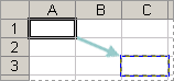
Move a Formula

To move a formula in Excel, simply use cut (CTRL + x) and paste (CTRL + v). Excel pros use the following trick to move a formula.

1. Select a cell with a formula.

2. Hover over the border of the selection. A four-sided arrow appears.

3. Click and hold the left mouse button.

4. Move the formula to the new position.

5. Release the left mouse button.

Exact Copy

To make an exact copy of a formula, without changing the cell references, execute the following easy steps.

1. Click in the formula bar and select the formula.

2. Press CTRL + c and press Enter.

3. Select another cell and press CTRL + v.

Result:

Conclusion: cell A3 and cell B3 contain the exact same formula.

Copy Magic

To make an exact copy of multiple formulas, repeat the previous steps for each formula. You can also use the following magic trick.

1. Select multiple formulas.

2. Replace all equal signs with xxx.

Result.

3. Use CTRL + c and CTRL + v to copy and paste the text strings.

4. Select the range B6:B10, hold down CTRL, select the range E6:E10 and replace all occurrences of ‘xxx’ with equal signs (the exact opposite of step 2).

Result.

Conclusion: cell B6 and cell E6 contain the exact same formula, cell B7 and cell E7 contain the exact same formula, etc.

Источник

See all How-To Articles

This tutorial demonstrates how to copy and paste exact formulas in Excel and Google Sheets.

Copy and Paste Exact Formula – Find & Replace Feature

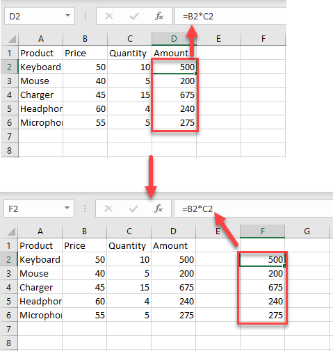
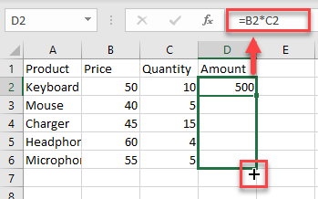
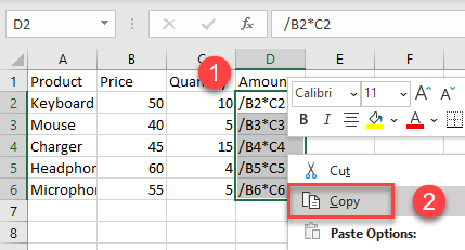
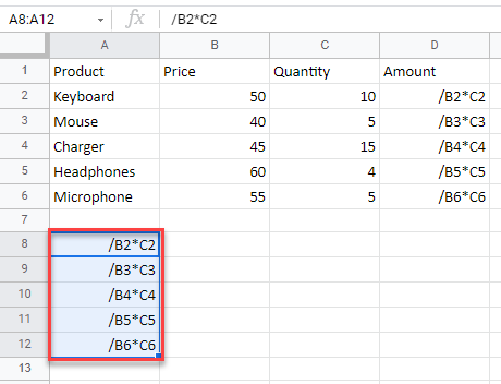
In the example below, you have an amount in Column D that is the product of values in Columns B and C. Now, say you want to copy the range (D2:D6) to another location, keeping the formulas, and without changing the cell references.

In cell D2, enter the formula:

=B2*C2

and drag it to the end of the range (D6).

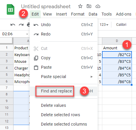
To copy and paste the exact formula without changing the cell references to another place in your sheet, you need to convert the formulas to text and then copy them. To do that, select the range with formulas you want to copy. Then, in the Ribbon, go to Home > Editing > Find & Select > Replace.

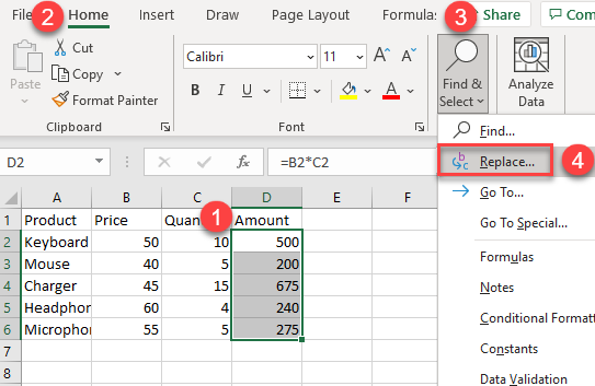
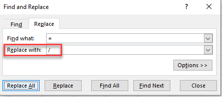
The Find and Replace dialog box will appear. In the Replace with: box, type any symbol that you want to use instead of = (equal sign). Then click on the Replace All button.

As a result, all the equal signs in the range you selected are replaced with the chosen symbol. Since the content in each cell no longer starts with “=”, it will be in text form.
Now, select that range, right-click it, and from the drop-down menu, choose Copy (or use the CTRL + C shortcut).

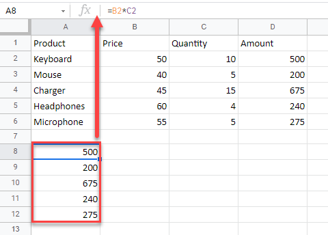
Then, select the place where you want to paste the range, right-click it, and under Paste Options click on the Paste icon (or you could use the CTRL + V shortcut).

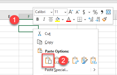
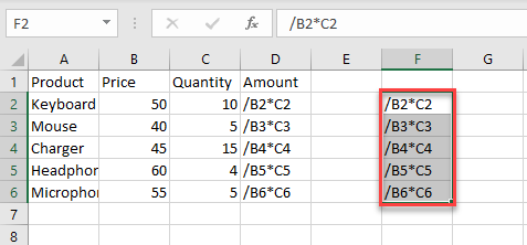
This pastes the range in Column F.

To convert the copied and pasted ranges back to formulas, select both ranges and in the Ribbon, go to Home > Find & Replace > Replace.

In the Find and Replace dialog box, (1) under Find what: enter the symbol you chose in Step 3, and (2) under Replace with: enter = (an equal sign). Then, (3) click the Replace All button.

After that, an information window will appear to inform you that all the replacements were made. To finish, just click OK.

As a result of Steps 1–9, you have the exact formula, copied from Column D and pasted to Column F, without changing cell references.

You can also use a macro to copy and paste the exact formula in Excel.

Copy and Paste Exact Formula – Absolute References

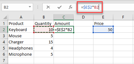
Another way to copy and paste a formula without changing references is to use absolute cell references. If you want a formula to consistently refer to a particular cell, regardless of where you copy or move that formula in the worksheet, you should use absolute cell references, which do not change when copied.

First, click on the cell where you want to enter a formula and type = (an equal sign) to begin. Then, select the cell you want to make an absolute reference and press F4:

=$E$2*B2

When done with the formula, press ENTER.

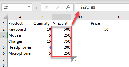
Then, copy the formula by dragging it down the column.

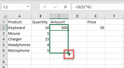
As a result, the formula is copied down the column, and the reference to cell E2 does not change.

Copy and Paste Exact Formula in Google Sheets

In Google Sheets, you can copy and paste the exact formula using absolute references and dragging by performing the same steps shown above for Excel (or copy from Excel).

To copy the exact formula with the Find and Replace feature, the steps are a bit different.

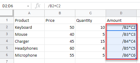
In the cell D3, enter the formula:

=B2*C2

and drag the fill handle down the cells you want to fill with formulas (D2:D6).

After that, (1) select the range and in the Menu, (2) click on Edit. From the drop-down menu, (3) choose to Find and replace.

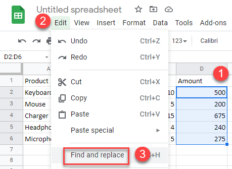
The Find and Replace dialog box will appear. (1) In the Find box, type = (an equal sign); and (2) in the Replace with box, type the symbol you want to replace “=” with. (3) Then indicate the specific range where you want to do the replacement, and (4) check the box next to the Also search within formulas. Finally, (5) click the Replace all button and (6) click Done.

As a result, all the = (equal signs) are replaced with the symbol you chose, and the range will no longer be read as formulas.

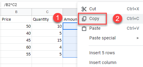
Now, select that range (D2:D6), right-click it, and click on Copy (or use the CTRL + C shortcut).

Select the place where you want to paste the range, right-click it and click on Paste (or use the CTRL + V shortcut).

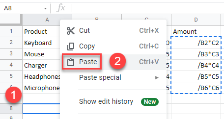
This pastes the (text) range in A8:A12.

To convert both the copied and pasted ranges back to formulas, , (1) select them and in the Menu, (2) click on Edit and (3) choose to Find and replace.

The Find and replace window will appear. (1) In the Find box, type the symbol you used in Step 3 (in this example, slash). (2) In the Replace with box, type = (an equal sign). (3) Then, specify the scope for the replacement (in this example, “This sheet”), and (4) check the box next to Also search within formulas. Finally, (5) click the Replace all button and (6) click Done.

As a result, you have the exact formula copied without changing cell references.

Источник

One of the great things about working digitally is that it can cut down on a lot of unnecessarily repetitive work. For example, if you must fill the same content into multiple cells in a spreadsheet, you can just copy and paste the values to save time.

Although, this can get a little tricky if you need to copy formulas. Luckily, Excel has several ways to copy and paste formulas. But, there are a couple of things you need to keep in mind when doing so.

Relative Cell References

Before we can jump into copying formulas, you need to know a little bit about how Excel references cells. Excel tracks the relation between the cells in the formula, not the actual cells.

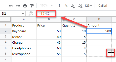
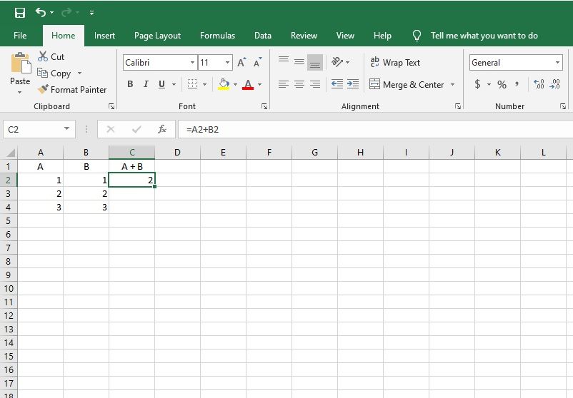
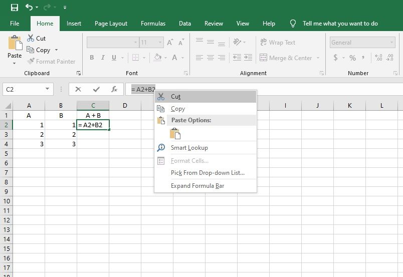
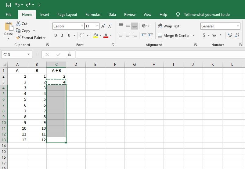
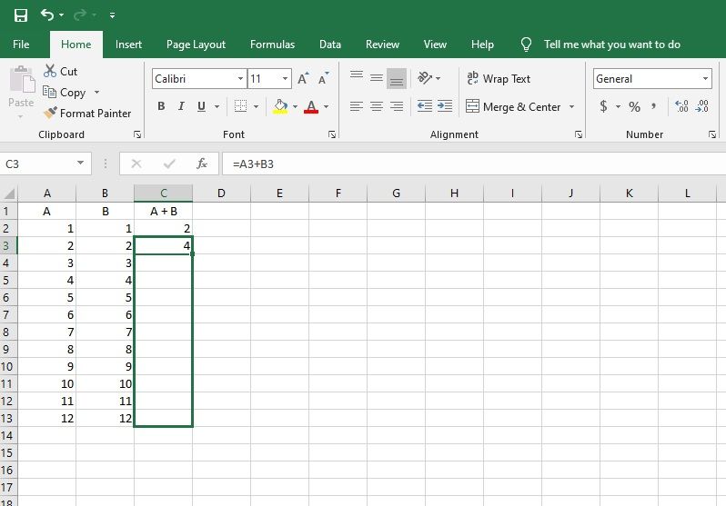
For example, in the image below, cell C2 contains the formula A2 + B2. But thanks to relative cell references, Excel reads this as: add the cell that is two places to the left to the cell that is one place to the left.

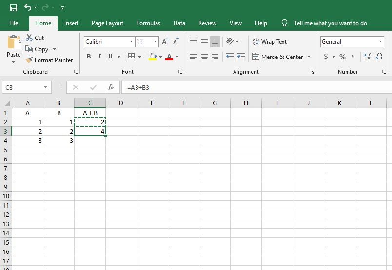
These relative cell references can be very handy. If you want to add the values on row 3 and 4 in the same way you did for row 2, all you have to do is copy the formula down without worrying about changing the rows yourself. Excel updates the rows in each formula so that the cells to the left of that add together.

However, sometimes you don’t want a cell’s location to change when you copy a formula.

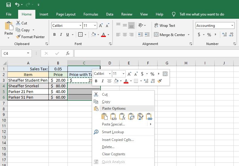
For example, let’s say you want to work out the sales tax on a series of products, as we’ve done below. If you add the sales tax to one cell, you want that cell to remain the same in the formula for each product. To do this, you need to tell that Excel the location of that cell is fixed, not relational. You do this with a $ sign in front of the row, column, or both.

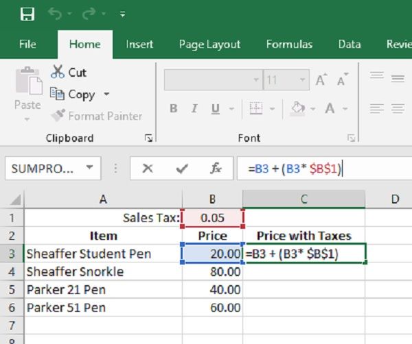
Adding the $ before the B tells Excel that no matter where we paste the formula, we want to look at the B column. To stop the row from changing, we also added a $ before the 1. Now, no matter where we paste the formula, it will always reference B1 for the tax value.

As we copy the formula down the column, the price location updates, but the sales tax location stays the same.

Using the F4 Keyboard Shortcut

There is a keyboard shortcut to toggle through a cell’s reference options. When you’re writing a formula and click on a cell, hit F4 to fix that cell. For example, if you click on B1 and press F4, it changes the reference to $B$1. If you press F4 again, the cell reference changes to B$1, then to $B1, and finally back to B1.

Copying and Pasting a Formula Manually

The most familiar way to copy and paste a formula is to copy and paste the formula text inside a cell. This is similar to how you would copy and paste text in Word.

Copy the text by selecting the cell and right-clicking the formula at the top of the screen. This brings up a popup with various options, select Copy. You can also use the copy button in the ribbon, which is located in the Clipboard section of the Home tab.

Then unselect the text by pressing the Return key. Finally, right-click the new cell you want to paste into and click on the clipboard icon or use the Paste button in the ribbon. You can also use the keyboard shortcut, Ctrl + C, to copy the highlighted text and Ctrl + V to paste it once you select a new cell.

This method is familiar, but not one of the best ways to copy a formula. If you had to copy a formula to multiple cells it would be time-consuming. This method also copies your exact text, so you don’t get the benefits of relative cell references we talked about above.

You should only use this method if you only need to copy the formula to a couple of places and you want the cells to remain exactly the same each time.

A Better Way to Copy a Formula in Excel

An easier way to copy the formula is to use copy and paste on the entire cell instead of just the text inside it. Click on the cell with the formula you wish to copy. Then copy it by either right-clicking on the cell, or using the keyboard shortcut Ctrl + C.

Once you copy the cell, it will have a dashed green border to show that you are currently copying it. Next, select the cell you want to paste the formula to. Then paste the formula by either right-clicking on the cell, or using the keyboard shortcut Ctrl + V.

This time, you’ll notice the formula uses relative cell references. Instead of A2 + B2, a formula on the row beneath becomes A3 + B3. Similarly, if you pasted the formula in the next column in the row beneath, it would update to B3 + C3.

How to Drag a Formula Down a Column or Across a Row

The method above can still be too time-consuming if you need to paste the same formula to multiple rows or columns. Luckily, there are two even quicker ways to do this.

First, you can copy the formula as you did above, but instead of pasting it to one cell, you can click and drag to select multiple cells and paste the formula to all of them by right-clicking any the cell or using the keyboard shortcut Ctrl + V.

The second way to paste the same formula to multiple rows is to drag it. At the bottom-right corner of a selected cell, you’ll see a green square. Click on that square and drag it over the cells you wish to copy the formula to. This is probably the quickest way to copy an Excel formula down a column or across a row.

Again, you’ll see that Excel updates the formula to use relative cell references for each row or column that changes.

Paste Special

One problem you may have when pasting a formula is that it also pastes any styling to the selected cells. Styling includes elements like the font size, cell outline, colors, or bold settings. Pasting the styling is inconvenient if you use alternate line colors or if you outlined your table.

To solve this, Excel introduced Paste Special.

Use Paste Special to paste just the formula without any of the styles that were added to the cell. To use Paste Special, right-click and select Paste Special from the popup menu.

A Recap of How to Copy and Paste Excel Formulas

Excel is optimized to reduce the number of repetitive tasks that you need to complete. Adding the same formula to multiple cells is quick and easy to do in Excel. You can copy and paste formula text, much like you would in a Word document. But if you want to take advantage of relative cell references, you’re better off using different methods.

A good way to copy a formula is by selecting the entire cell with the formula and copying that. If you need to copy a formula down a column or across a row, you can also drag the cell across the area you want to copy it to, which is much quicker.

Both methods allow you to copy a formula to multiple cells quickly. Next time you create a spreadsheet, remember to try it out and save yourself some precious time.

Источник