
Excel for Microsoft 365 for Mac Excel 2021 for Mac Excel 2019 for Mac Excel 2016 for Mac Excel for Mac 2011 More…Less
You can copy and paste specific cell contents or attributes (such as formulas, formats, comments, and validation). By default, if you use the Copy  and Paste
  icons (or
  + C and + V), all attributes are copied. To pick a specific paste option, you can either use a Paste menu option or select Paste Special, and pick an option from the Paste Special box. Attributes other than what you select are excluded when you paste.

Paste menu options
-
Select the cells that contain the data or other attributes that you want to copy.
-
On the Home tab, click Copy
 .
. -
Click the first cell in the area where you want to paste what you copied.
-
On the Home tab, click the arrow next to Paste, and then do any of the following. The options on the Paste menu will depend on the type of data in the selected cells:
|
Select |
To paste |
|---|---|
|
Paste |
All cell contents and formatting, including linked data. |
|
Formulas |
Only the formulas. |
|
Formulas & Number Formatting |
Only formulas and number formatting options. |
|
Keep Source Formatting |
All cell contents and formatting. |
|
No Borders |
All cell contents and formatting except cell borders. |
|
Keep Source Column Widths |
Only column widths. |
|
Transpose |
Reorients the content of copied cells when pasting. Data in rows is pasted into columns and vice versa. |
|
Paste Values |
Only the values as displayed in the cells. |
|
Values & Number Formatting |
Only the values and number formatting. |
|
Values & Source Formatting |
Only the values and number color and font size formatting. |
|
Formatting |
All cell formatting, including number and source formatting. |
|
Paste Link |
Link the pasted data to the original data. When you paste a link to the data that you copied, Excel enters an absolute reference to the copied cell or range of cells in the new location. |
|
Paste as Picture |
A copy of the image. |
|
Linked Picture |
A copy of the image with a link to the original cells (if you make any changes to the original cells those changes are reflected in the pasted image). |
|
Column widths |
Paste the width of one column or range of columns to another column or range of columns. |
|
Merge conditional formatting |
Combine conditional formatting from the copied cells with conditional formatting present in the paste area. |
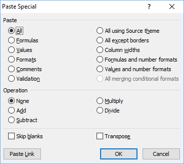
Paste Special options
-
Select the cells that contain the data or other attributes that you want to copy.
-
On the Home tab, click Copy
. -
Click the first cell in the area where you want to paste what you copied.
-
On the Home tab, click the arrow next to Paste, and then select Paste Special.
-
Select the options you want.
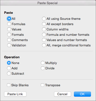
Paste options
|
Select |
To paste |
|---|---|
|
All |
All cell contents and formatting, including linked data. |
|
Formulas |
Only the formulas. |
|
Values |
Only the values as displayed in the cells. |
|
Formats |
Cell contents and formatting. |
|
Comments |
Only comments attached to the cell. |
|
Validation |
Only data validation rules. |
|
All using Source theme |
All cell contents and formatting using the theme that was applied to the source data. |
|
All except borders |
Cell contents and formatting except cell borders. |
|
Column widths |
The width of one column or range of columns to another column or range of columns. |
|
Formulas and number formats |
Only formulas and number formatting. |
|
Values and number formats |
Only values and number formatting options from the selected cells. |
|
All, merge conditional formats |
Combine conditional formatting from the copied cells with conditional formatting present in the paste area. |
Operation options
The Operation options mathematically combine values between the copy and paste areas.
|
Click |
To |
|---|---|
|
None |
Paste the contents of the copy area without a mathematical operation. |
|
Add |
Add the values in the copy area to the values in the paste area. |
|
Subtract |
Subtract the values in the copy area from the values in the paste area. |
|
Multiply |
Multiply the values in the paste area by the values in the copy area. |
|
Divide |
Divide the values in the paste area by the values in the copy area. |
Other options
|
Click |
To |
|
Skip Blanks |
Avoid replacing values or attributes in your paste area when blank cells occur in the copy area. |
|
Transpose |
Reorients the content of copied cells when pasting. Data in rows is pasted into columns and vice versa. |
|
Paste Link |
If data is a picture, links to the source picture. If the source picture is changed, this one will change too. |
Tip: Some options are available both on the Paste menu and in the Paste Special dialog box. The option names might vary a bit but the results are the same.
-
Select the cells that contain the data or other attributes that you want to copy.
-
On the Standard toolbar, click Copy
. -
Click the first cell in the area where you want to paste what you copied.
-
On the Home tab, under Edit, click Paste, and then click Paste Special.
-
On the Paste Special dialog, under Paste, do any of the following:
Click
To
All
Paste all cell contents and formatting, including linked data.
Formulas
Paste only the formulas as entered in the formula bar.
Values
Paste only the values as displayed in the cells.
Formats
Paste only cell formatting.
Comments
Paste only comments attached to the cell.
Validation
Paste data validation rules for the copied cells to the paste area.
All using Source theme
Paste all cell contents and formatting using the theme that was applied to the source data.
All except borders
Paste all cell contents and formatting except cell borders.
Column widths
Paste the width of one column or range of columns to another column or range of columns.
Formulas and number formats
Paste only formulas and number formatting options from the selected cells.
Values and number formats
Paste only values and number formatting options from the selected cells.
Merge conditional formatting
Combine conditional formatting from the copied cells with conditional formatting present in the paste area.
To mathematically combine values between the copy and paste areas, in the Paste Special dialog box, under Operation, click the mathematical operation that you want to apply to the data that you copied.
Click
To
None
Paste the contents of the copy area without a mathematical operation.
Add
Add the values in the copy area to the values in the paste area.
Subtract
Subtract the values in the copy area from the values in the paste area.
Multiply
Multiply the values in the paste area by the values in the copy area.
Divide
Divide the values in the paste area by the values in the copy area.
Additional options determine how blank cells are handled when pasted, whether copied data is pasted as rows or columns, and linking the pasted data to the copied data.
Click
To
Skip blanks
Avoid replacing values in your paste area when blank cells occur in the copy area.
Transpose
Change columns of copied data to rows, or vice versa.
Paste Link
Link the pasted data to the original data. When you paste a link to the data that you copied, Excel enters an absolute reference to the copied cell or range of cells in the new location.
Note: This option is available only when you select All or All except borders under Paste in the Paste Special dialog box
 .
.
Tip: In Excel for Mac version 16.33 or higher, the «paste formatting», «paste formulas», and «paste values» actions can be added to your quick-access toolbar (QAT) or assigned to custom key combinations. For the keyboard shortcuts, you’ll need to assign a key combination that isn’t already being used to open the Paste Special dialog.
See Also
Move or copy a sheet
Move or copy cells, rows, or columns
Customize the Ribbon and toolbars in Office for Mac
Create a custom keyboard shortcut for Office for Mac
Need more help?
I’m trying to copy the cell contents into the clipboard.
I’ve read and tried the exact example provided in the Excel 2007 Help file. However for some reason the DataObject object is not valid. So the example:
Dim MyData As DataObject

Private Sub CommandButton1_Click()
    Set MyData = New DataObject

    MyData.SetText TextBox1.Text
    MyData.PutInClipboard

    TextBox2.Paste
End Sub

Private Sub UserForm_Initialize()
    TextBox1.Text = "Move this data to a " _
        & "DataObject, to the Clipboard, then to " _
        & "TextBox2!"
End Sub
Does not work in my case. I’ve searched for a good while now and I can not find an answer to why the DataObject object is not available.
Here is my code:
Dim MyData As DataObject

Private Sub Worksheet_Change(ByVal Target As Range)
    If ActiveCell.Column = 3 Then
        Set MyData = New DataObject
        MyData.SetText ActiveCell.Offset(-1, -1).Text
        MyData.PutInclipboard
    End If
End Sub
Error on Compile is: «User-Defined type not defined» and it highlights the «MyData As DataObject» line.
Is there another method to simply copying the text in a cell to the clipboard?
One of the most common tasks in Excel is to copy a cell. To copy a cell, as we all know, use the command CTRL+C or by right-clicking on it and selecting Copy. But when you need to do cell copying more often, it wastes a lot of time. We can create a shortcut for copying the cells using the VB code. The shortcut will be to copy the cell with a single click.
This tutorial will help you understand how we can automatically copy a cell to the clipboard with a single click in Excel.
Automatically Copy a Cell to Clipboard with a Single Click
Here we will insert the VBA code for the sheet, then return to the sheet to complete our task. Let us see a straightforward process to see how we can automatically copy a cell to the clipboard with a single click in Excel.
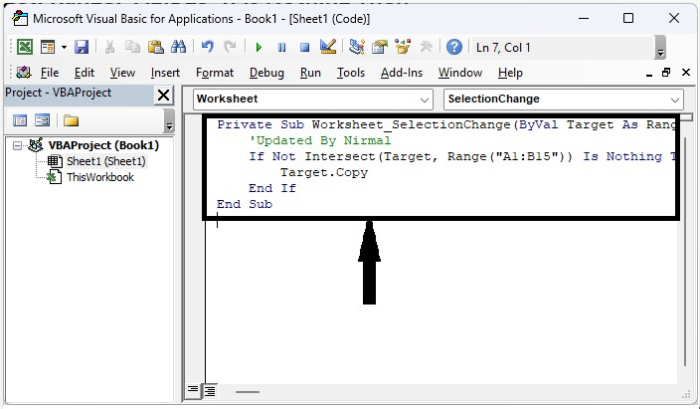
Step 1
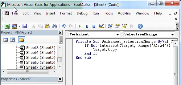
Let us consider a new Excel sheet and use the command «Alt + F11» to open the vba application, then type the below-mentioned programme into the text box as shown in the below image.
Example
Private Sub Worksheet_SelectionChange(ByVal Target As Range)
   'Updated By Nirmal
   If Not Intersect(Target, Range("A1:B15")) Is Nothing Then
      Target.Copy
   End If
End Sub
In the code, the range A1:B15 is the range of cells where our code will work. We can use this code to copy one cell or multiple cells at once.
Step 2
Now save the workbook as a macro-enabled workbook and close the vba application using the command «Alt + Q». From now on, every time we click on a cell that is mentioned in the range of code, the data in that cell will be copied automatically. When we select any cell in the range, then it will be copied automatically.
Conclusion
In this tutorial, we used a simple example to demonstrate how we can automatically copy a cell to the clipboard with a single click in Excel.
This post will teach you how to use the Excel VBA macro code to copy a Cell to clipboard with only single click in Excel. How do I automatically copy the content of cell to Clipboard while clicking on the Cell or just single click on the cell in Microsoft Excel 2016, 2013 and older versions.
Normally, to copy a cell to the clipboard, you need to select a Cell firstly, press Ctrl + C shortcut to copy the content into clipboard. Whether there is any other ways to omit one or two steps to copy a cell to clipboard. Of course yes, you can try to write an Excel Macro code to copy cell content into clipboard while you click on that cell.
Let’s see the below detailed steps:
1# open your worksheet contain cells that you want to copy them to clipboard.
2# right click on the sheet tab, then select View Code menu from the pop-up menu list.
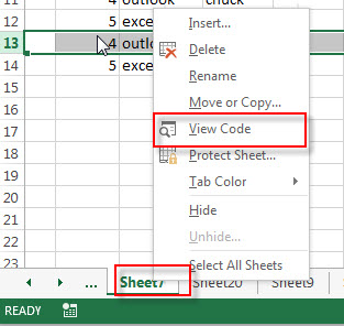
3# then the “Visual Basic Editor” window will appear
4# paste the below VBA code into the code window. Then clicking “Save” button.
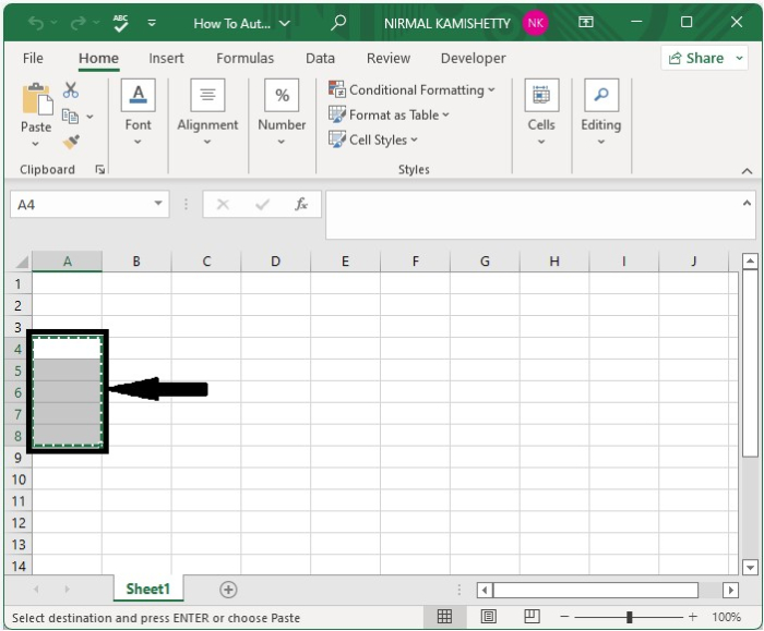
Private Sub Worksheet_SelectionChange(ByVal Target As Range)
    If Not Intersect(Target, Range("A1:A4")) Is Nothing Then
        Target.Copy
    End If
End Sub
5# try to click cell A1 to A4, you will see that all Cell that you clicked are copied to clipboard automatically.
If you want to use this VBA macro code, just need to update the Range as you need.
Speed Up Copying and Pasting Using These Great Tricks and Shortcuts in Microsoft Excel
by Avantix Learning Team | Updated April 10, 2021
Applies to: Microsoft® Excel® 2013, 2016, 2019 and 365 (Windows)
It’s surprising how much time you can save with a few tricks and shortcuts for copying and pasting in Microsoft Excel. Here are 10 useful copy and paste shortcuts for Excel users.
Recommended article: 10 Excel Data Entry Tricks and Shortcuts Every User Should Know
Do you want to learn more about Excel? Check out our virtual classroom or live classroom Excel courses >
For the following examples, if you are dragging, clicking or double-clicking, use the left mouse button.
1. Copying and pasting using Ctrl + C and Ctrl + V
The most popular shortcut for copying and pasting can be used in Excel and other programs as well. In Excel, select the cells you want to copy and press Ctrl + C. Click the top left cell where you wish to paste and press Ctrl + V. The copied selection is saved in the Clipboard so you can continue pressing Ctrl + V in different locations if you want to make multiple copies of the selection.
2. Copying and pasting using Paste Special
Paste Special is a very useful tool in Excel. Many options from Paste Special appear when you copy and then right-click a cell (such as values). However, you can also access Paste Special using your keyboard.
Select the cells you want to copy and press Ctrl + C. Click the top left cell where you wish to paste and press Ctrl + Alt + V. The Paste Special dialog box appears. Select an option (such as Values) and click OK.
3. Copying formulas down quickly
Instead of dragging the Fill handle on the bottom right corner of a cell to copy a formula down, select the cell with the formula you want to copy and double-click the handle on the bottom right corner. Excel will copy the formula down as long as there is data on the left.
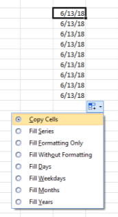
4. Copying a date
It’s common for Excel users to drag the Fill handle on the bottom right corner of a cell to copy a date. However, if you drag the Fill handle of a cell containing a date, Excel assumes you want to generate a date series. If this occurs and you want to copy the date, click the Smart Tag that appears after you drag the Fill handle and select Copy Cells from the menu.
5. Copying using Drag and Drop
You can use Excel’s Drag and Drop pointer to copy a cell or range of cells. Simply select a cell or a range of cells and point to the border of the cell or range (not the corner). The pointer changes to the Drag and Drop pointer. Press Ctrl and drag the border of the cell or range to a new location. Release the mouse button and then release Ctrl. Excel will create a copy in the new location.
You can also use the Drag and Drop pointer to copy to another sheet. Select a cell or a range of cells and point to the border of the cell or range. The pointer changes to the Drag and Drop pointer. Press Ctrl + Alt and drag the border of the cell or range to a sheet tab to activate the sheet and then drag to a new location. Release the mouse button and then release Ctrl + Alt. Excel will create a copy in the new location on the other sheet.
6. Copying from the cell above
To copy the data or formula from the cell above, click the cell below the cell you want to copy and press Ctrl + ‘ (apostrophe) or Ctrl + D.
7. Copying the value only from the cell above
To copy the value only (not the formula) from the cell above, click the cell below the cell you want to copy and press Ctrl + Shift + ‘ (apostrophe).
8. Copying from the cell to the left
To copy the data or formula from the cell to the left, click in the cell to the right of the cell and you want to copy and press Ctrl + R.
9. Copying formatting
To copy formatting from one cell to another:
- Click the cell with the formatting you want to copy.
- Click the Home tab in the Ribbon.
- Click the Format Painter in the Clipboard group.
- Click the cell to which you want to copy the formatting.
The Format Painter appears on the left in the Home tab in the Ribbon:
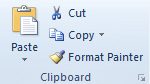
To copy formatting from one cell to many other cells:
- Click the cell with the formatting you want to copy.
- Click the Home tab in the Ribbon.
- Double-click the Format Painter in the Clipboard group.
- Click the cells to which you want to copy the formatting.
- Press ESC or click the Format Painter to turn it off.
10. Copying a sheet
To quickly copy a sheet, point to the sheet tab you want to copy and then press Ctrl and drag the sheet to the right or left of the sheet tab. A sheet icon with a plus sign appears. Release the mouse button and then release Ctrl when the copy is in the desired location.
Subscribe to get more articles like this one
Did you find this article helpful? If you would like to receive new articles, join our email list.
More resources
How to Quickly Delete Blank Rows in Excel (5 Ways)
How to Fill or Replace Blank Cells in Excel with a Value from a Cell Above
How to Use Flash Fill in Excel to Clean or Extract Data (Beginner’s Guide)
How to Use Conditional Formatting in Excel to Highlight Dates Before Today (3 Ways)
Related courses
Microsoft Excel: Intermediate / Advanced
Microsoft Excel: Data Analysis with Functions, Dashboards and What-If Analysis Tools
Microsoft Excel: Introduction to Visual Basic for Applications (VBA)
VIEW MORE COURSES >
Our instructor-led courses are delivered in virtual classroom format or at our downtown Toronto location at 18 King Street East, Suite 1400, Toronto, Ontario, Canada (some in-person classroom courses may also be delivered at an alternate downtown Toronto location). Contact us at info@avantixlearning.ca if you’d like to arrange custom instructor-led virtual classroom or onsite training on a date that’s convenient for you.
Copyright 2023 Avantix® Learning
Microsoft, the Microsoft logo, Microsoft Office and related Microsoft applications and logos are registered trademarks of Microsoft Corporation in Canada, US and other countries. All other trademarks are the property of the registered owners.
Avantix Learning |18 King Street East, Suite 1400, Toronto, Ontario, Canada M5C 1C4 | Contact us at info@avantixlearning.ca
Обычно при копировании ячейки в буфер обмена вам нужно сначала выбрать ячейку, а затем нажать кнопку Ctrl + C ключ, чтобы скопировать его. Как автоматически скопировать ячейку, просто щелкнув по ней без нажатия горячих клавиш? Метод, описанный в этой статье, может вам помочь.
Автоматически копировать ячейку в буфер обмена, щелкая с кодом VBA
Автоматически копировать ячейку в буфер обмена, щелкая с кодом VBA
Следующий код VBA поможет скопировать ячейку в буфер обмена, просто щелкнув ее в Excel. Пожалуйста, сделайте следующее.
1. Откройте рабочий лист, ячейки которого нужно автоматически скопировать в буфер обмена, щелкните правой кнопкой мыши вкладку листа и выберите Просмотреть код из контекстного меню. Смотрите скриншот:
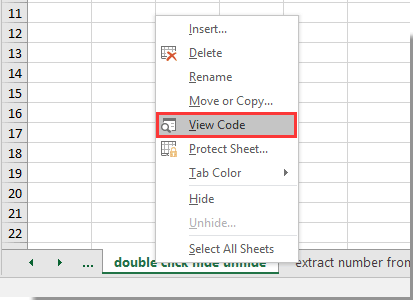
2. В дебюте Microsoft Visual Basic для приложений окна, скопируйте код VBA в окно кода.
Код VBA: автоматическое копирование ячейки в буфер обмена, щелкнув
Private Sub Worksheet_SelectionChange(ByVal Target As Range)
    If Not Intersect(Target, Range("A1:A9")) Is Nothing Then
        Target.Copy
    End If
End SubNote: In the code, A1:A9 is the cells you will copy to clipboard automatically. Please change it based on your need.
3. Press the Alt + Q keys to close the Microsoft Visual Basic for Applications window.
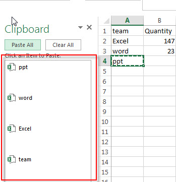
When clicking on any cell of range A1:A9, the cell will be copied automatically to the clipboard as below screenshot shown.

And then, you can select a destination cell and press Enter key to paste the copied contents.
Related articles:
- How to copy cells data with row height and column width in Excel?
- How to auto copy and paste cell in current sheet or from one sheet to another in Excel?
- How to disable cut, copy and paste functions in Excel?
- How to copy only borders of selected range in Excel?
The Best Office Productivity Tools
Kutools for Excel Solves Most of Your Problems, and Increases Your Productivity by 80%
- Reuse: Quickly insert complex formulas, charts and anything that you have used before; Encrypt Cells with password; Create Mailing List and send emails…
- Super Formula Bar (easily edit multiple lines of text and formula); Reading Layout (easily read and edit large numbers of cells); Paste to Filtered Range…
- Merge Cells/Rows/Columns without losing Data; Split Cells Content; Combine Duplicate Rows/Columns… Prevent Duplicate Cells; Compare Ranges…
- Select Duplicate or Unique Rows; Select Blank Rows (all cells are empty); Super Find and Fuzzy Find in Many Workbooks; Random Select…
- Exact Copy Multiple Cells without changing formula reference; Auto Create References to Multiple Sheets; Insert Bullets, Check Boxes and more…
- Extract Text, Add Text, Remove by Position, Remove Space; Create and Print Paging Subtotals; Convert Between Cells Content and Comments…
- Super Filter (save and apply filter schemes to other sheets); Advanced Sort by month/week/day, frequency and more; Special Filter by bold, italic…
- Combine Workbooks and WorkSheets; Merge Tables based on key columns; Split Data into Multiple Sheets; Batch Convert xls, xlsx and PDF…
- More than 300 powerful features. Supports Office / Excel 2007-2021 and 365. Supports all languages. Easy deploying in your enterprise or organization. Full features 30-day free trial. 60-day money back guarantee.
")
Read More… Free Download… Purchase…
Office Tab Brings Tabbed interface to Office, and Make Your Work Much Easier
- Enable tabbed editing and reading in Word, Excel, PowerPoint, Publisher, Access, Visio and Project.
- Open and create multiple documents in new tabs of the same window, rather than in new windows.
- Increases your productivity by 50%, and reduces hundreds of mouse clicks for you every day!
")
Read More… Free Download… Purchase…
Comments (3)
No ratings yet. Be the first to rate!
") Copy and paste are 2 of the most common Excel operations. Copying and pasting a cell range (usually containing data) is an essential skill you’ll need when working with Excel VBA.
Copy and paste are 2 of the most common Excel operations. Copying and pasting a cell range (usually containing data) is an essential skill you’ll need when working with Excel VBA.
You’ve probably copied and pasted many cell ranges manually. The process itself is quite easy.
Well…
You can also copy and paste cells and ranges of cells when working with Visual Basic for Applications. As you learn in this Excel VBA Tutorial, you can easily copy and paste cell ranges using VBA.
However, for purposes of copying and pasting ranges with Visual Basic for Applications, you have a variety of methods to choose from.
My main objective with this Excel tutorial is to introduce to you the most important VBA methods and properties that you can use for purposes of carrying out these copy and paste activities with Visual Basic for Applications in Excel. In addition to explaining everything you need to know in order to start using these different methods and properties to copy and paste cell ranges, I show you 8 different examples of VBA code that you can easily adjust and use immediately for these purposes.
The following table of contents lists the main topics (and VBA methods) that I cover in this blog post. Use the table of contents to navigate to the topic that interests you at the moment, but make sure to read all sections 😉 .
Let’s start by taking a look at some information that will help you to easily modify the source and destination ranges of the sample macros I provide in the sections below (if you need to).
Scope Of Macro Examples In This Tutorial And How To Modify The Source Or Destination Cells
As you’ve seen in the table of contents above, this Excel tutorial covers several different ways of copying and pasting cells ranges using VBA. Each of these different methods is accompanied by, at least, 1 example of VBA code that you can adjust and use immediately.
All of these macro examples assume that the sample workbook is active and the whole operation takes place on the active workbook. Furthermore, they are designed to copy from a particular source worksheet to another destination worksheet within that sample workbook.
You can easily modify these behaviors by adjusting the way in which the object references are built. You can, for example, copy a cell range to a different worksheet or workbook by qualifying the object reference specifying the destination cell range.
Similar comments apply for purposes of modifying the source and destination cell ranges. More precisely, to (i) copy a different range or (ii) copy to a different destination range, simply modify the range references.
For example, in the VBA code examples that I include throughout this Excel tutorial, the cell range where the source data is located is referred to as follows:
Worksheets("Sample Data").Range("B5:M107")
This reference isn’t a fully qualified object reference. More precisely, it assumes that the copying and pasting operations take place in the active workbook.
The following reference is the equivalent of the above, but is fully qualified:
Workbooks("Book1.xlsm").Worksheets("Sample Data").Range("B5:M107")
This fully qualified reference doesn’t assume that Book1.xlsm is the active workbook. Therefore, the reference works appropriately regardless of which Excel workbook is active.
I explain how to work with object references in detail in The Essential Guide To Excel’s VBA Object Model And Object References. Similarly, I explain how to work with cell ranges in Excel’s VBA Range Object And Range Object References: The Tutorial for Beginners. I suggest you refer to these posts if you feel you need to refresh your knowledge about these topics, or if you’re not familiar with them. They will probably help you to better understand this Excel tutorial and how to modify the sample macros I include here.
You’ll also notice that within the VBA code examples that I include in this Excel tutorial, I always qualify the references up to the level of the worksheet. Strictly speaking, this isn’t always necessary. In fact, when implementing similar code in your VBA macros, you may want to modify the references by, for example:
- Using variables.
- Further simplifying the object references (not qualifying them up to the level of the worksheet).
- Using the With… End With statement.
The reason I’ve decided to keep references qualified up to the level of the worksheet is because the focus of this Excel tutorial is on how to copy and paste using VBA. Not on simplifying references or using variables, which are topics I cover in separate blog posts, such as those I link to above (and which I suggest you take a look at).
The Copy Command In Excel’s Ribbon
Before we go into how to copy a range using Visual Basic for Applications, let’s take a quick look at Excel’s ribbon:
Perhaps one of the most common used buttons in the Ribbon is “Copy”, within the Home tab.

When you think about copying ranges in Excel, you’re probably referring to the action carried out by Excel when you press this button: copying the current active cell or range of cells to the Clipboard.
You may have noticed, however, that the Copy button isn’t just a simple button. It’s actually a split button:
I explain how you can automate the functions of both of these commands in this Excel tutorial. More precisely:
- If you want to work with the regular Copy command, you’ll want to read more about the Range.Copy method, which I explain in the following section.
- If you want to use the Copy as Picture command, you’ll be interested in the Range.CopyPicture method, which I cover below.
Let’s start by taking a look at…
Excel VBA Copy Paste With The Range.Copy Method
The main purpose of the Range.Copy VBA method is to copy a particular range.
When you copy a range of cells manually by, for example, using the “Ctrl + C” keyboard shortcut, the range of cells is copied to the Clipboard. You can use the Range.Copy method to achieve the same thing.
However, the Copy method provides an additional option:
Copying the selected range to another range. You can achieve this by appropriately using the Destination parameter, which I explain in the following section.
In other words, you can use Range.Copy for copying a range to either of the following:
- The Clipboard.
- A certain range.
The Range.Copy VBA Method: Syntax And Parameters
The basic syntax of the Range.Copy method is as follows:
expression.Copy(Destination)
“expression” is the placeholder for the variable representing the Range object that you want to copy.
The only parameter of the Copy VBA method is Destination. This parameter is optional, and allows you to specify the range to which you want to copy the copied range. If you omit the Destination parameter, the copied range is simply copied to the Clipboard.
This means that the appropriate syntax you should use for the Copy method (depending on your purpose) is as follows:
- To copy a Range object to the Clipboard, omit the Destination parameter. In such a case, use the following syntax:
expression.Copy
- To copy the Range object to another (the destination) range, use the Destination parameter to specify the destination range. This means that you should use the following syntax:
expression.Copy(Destination)
Let’s take a look at how you can use the Range.Copy method to copy and paste a range of cells in Excel:
Macro Examples #1 And #2: The VBA Range.Copy Method
This Excel VBA Copy Paste Tutorial is accompanied by an Excel workbook containing the data and macros I use. You can get immediate free access to this workbook by clicking the button below.

For this particular example, I’ve created the following table. This table displays the sales of certain items (A, B, C, D and E) made by 100 different sales managers in terms of units and total Dollar value. The first row (above the main table), displays the unit price for each item. The last column displays the total value of the sales made by each manager.

Macro Example #1: Copy A Cell Range To The Clipboard
First, let’s take a look at how you can copy all of the items within the sample worksheet (table and unit prices) to the Clipboard. The following simple macro (called “Copy_to_Clipboard”) achieves this:

This particular Sub procedure is made out of the following single statement:
Worksheets("Sample Data").Range("B5:M107").Copy
This statement is made up by the following 2 items:
Let’s take a look at this macro in action. Notice how, once I execute the Copy_to_Clipboard macro, the copied range of cells is surrounded by the usual dashed border that indicates that the range is available for pasting.
After executing the macro, I go to another worksheet and paste all manually. As a last step, I autofit the column width to ensure that all the data is visible.

Even though the sample Copy_to_Clipboard macro does what it’s supposed to do and is a good introduction to the Range.Copy method, it isn’t very powerful. It, literally, simply copies the relevant range to the Clipboard. You don’t really need a macro to do only that.
Fortunately, as explained above, the Range.Copy method has a parameter that allows you to specify the destination of the copied range. Let’s use this to improve the power of the sample macro:
Macro Example #2: Copy A Cell Range To A Destination Range
The following sample Sub procedure (named “Copy_to_Range”) takes the basic Copy_to_Clipboard macro used as example #1 above and adds the Destination parameter.

Even though it isn’t the topic of this Excel tutorial, I include an additional statement that uses the Range.AutoFit method.

Let’s take a closer look at each of the lines of code within this sample macro:
Line #1: Worksheets(“Sample Data”).Range(“B5:M107”).Copy
This is, substantially, the sample “Copy_to_Clipboard” macro which I explain in the section above.
More precisely, this particular line uses the Range.Copy method for purposes of copying the range of cells cells B5 and M107 of the worksheet called “Sample Data”.
However, at this point of the tutorial, our focus isn’t in the Copy method itself but rather in the Destination parameter which appears in…
Line #2: Destination:=Worksheets(“Example 2 – Destination”).Range(“B5:M107”)
You use the Destination parameter of the Range.Copy method for purposes of specifying the destination range in which to which the copied range of cells should be copied. In this particular case, the destination range is cells B5 to M107 of the worksheet named “Example 2 – Destination”, as shown in the image below:

As I explain above, you can easily modify this statement for purposes of specifying a different destination. For example, for purposes of specifying a destination range in a different Excel workbook, you just need to qualify the object reference.
Line #3: Worksheets(“Example 2 – Destination”).Columns(“B:M”).AutoFit
As anticipated above, this statement isn’t absolutely necessary for the sample macro to achieve its main purpose of copying the copied range in the destination range. Its purpose is solely to autofit the column width of the destination range.
For these purposes, I use the Range.Autofit method. The syntax of this method is as follows:
expression.AutoFit
In this particular case, “expression” represents a Range object, and must be either (i) a range of 1 or more rows, or (ii) a range of 1 or more columns. In the Copy_to_Range macro example, the Range object is columns B through M of the worksheet titled “Example 2 – Destination”. The following image shows how this range is specified within the VBA code.

The following image shows the results obtained when executing the Copy_to_Range macro. Notice how this worksheet looks substantially the same as the source worksheet displayed above.

If you were to compare the results obtained when copying a range to the Clipboard (example #1) with the results obtained when copying the range to a destination range (example #2), you may conclude that the general rule is that one should always use the Destination parameter of the Copy method.
To a certain extent, this is generally true and some Excel authorities generally discourage using the Clipboard. However, the choice between copying to the Clipboard or copying to a destination range isn’t always so straightforward. Let’s take a look at why this is the case:
The Range.Copy VBA Method: When To Copy To The Clipboard And When To Use The Destination Parameter
In my opinion, if you can achieve your purposes without copying to the Clipboard, you should simply use the Destination parameter of the Range.Copy method.
Using the Destination parameter is, generally, more efficient that copying to the Clipboard and then using the Range.PasteSpecial method or the Worksheet.Paste method (both of which I explain below). Copying to the Clipboard and pasting (with the Range.PasteSpecial or Worksheet.Paste methods) involves 2 steps:
- Copying.
- Pasting.
This 2-step process (usually):
- Increases the procedure’s memory requirements.
- Results in (slightly) less efficient procedures.
I explain this argument further in example #4 below, which introduces the Worksheet.Paste method. The Worksheet.Paste method is one of the VBA methods you’d use for purposes of pasting the data that you’ve copied to the Clipboard with the Range.Copy method.
Avoiding the Clipboard whenever possible may be a good idea to reduce the risks of data loss or leaks of information whenever another application is using the Clipboard at the same time. Some users report unpredictable Clipboard behavior in certain cases.
Considering this arguments, you probably understand why I say that, if you can avoid the Clipboard, you probably should.
However, using the Range.Copy method with the Destination parameter may not be the most appropriate solution always. For purposes of determining when the Destination parameter allows you to achieve the purpose you want, it’s very important that you’re aware of how the Range.Copy method works, particularly what it can (and can’t do). Let’s see an example of what I mean:
If you go back to the screenshots showing the results of executing the sample macros #1 (Copy_to_Clipboard) and #2 (Copy_to_Range), you’ll notice that the end result is that the destination worksheet looks pretty much the same as the source worksheet.
In other words, Excel copies and pastes all (for ex., values, formulas, formats).
In some cases, this is precisely what you want. However:
In other cases, this is precisely what you don’t want. Take a look, for example, at the following Sub procedure:

At first glance, this is the Copy_to_Range macro that I introduce and explain in the section above. Notice, however, that I’ve changed the Destination parameter. More precisely, in this version of the Copy_to_Range macro, the top-left cell of the destination range is cell B1 (instead of B5, as it was originally) of the “Example 2 – Destination” worksheet.

The following GIF shows what happens when I execute this macro. The worksheet shown is the destination “Example 2 – Destination” worksheet, and I’ve enabled iterative calculations (I explain to you below why I did this).

As you can see immediately, there’s something wrong. The total sales for all items are, clearly, inaccurate.

The reason for this is that, in the original table, I used mixed references in order to refer to the unit prices of the items. Notice, for example, the formula used to calculate the total sales of Item A made by Sarah Butler (the first Sales Manager in the table):

These formulas aren’t a problem as long as the destination cells are exactly the same as the source cells. This is the case in both examples #1 and #2 above where, despite the worksheet changing, the destination continues to be cells B5 to M107. That guarantees that the mixed references continue to point to the right cell.
However, once the destination range changes (as in the example above), the original mixed references wreak havoc on the worksheet. Take a look, for example, at the formula used to calculate the total sales of Item B by Sales Manager Walter Perry (second in the table):

The formula doesn’t use the unit price of Item B (which appears in cell F1) to calculate the sales. Instead, it uses cell F5 as a consequence of the mixed references copied from the source worksheet. This results in (i) the wrong result and (ii) a circular reference.
By the way, if you’re downloading the sample workbook that accompanies this Excel tutorial, it will have circular references.
In such (and other similar) cases, you may not want to rely solely on the Range.Copy method with the Destination parameter. In other words: There are cases where you don’t want to copy and paste all the contents of the source cell range. There are, for example, cases where you may want to:
- Copy a cell range containing formulas; and
- Paste values in the destination cell range.
This is precisely what happens in the case of the example above. In such a situation, you may want to paste only the values (no formulas).
For purposes of controlling what is copied in a particular destination range when working with VBA, you must understand the Range.PasteSpecial method. Let’s take a look at it:
Excel VBA Copy Paste With The Range.PasteSpecial Method
Usually, whenever you want to control what Excel copies in a particular destination range, you rely on the Paste Special options. You can access these options, for example, through the Paste Special dialog box.

When working with Visual Basic for Applications, you usually rely on the Range.PasteSpecial method for purposes of controlling what is copied in the destination range.
Generally speaking, the Range.PasteSpecial method allows you to paste a particular Range object from the Clipboard into the relevant destination range. This, by itself, isn’t particularly exciting.
The power of the Range.PasteSpecial method comes from its parameters, and the ways in which they allow you to further determine the way in which Excel carries out the pasting. Therefore, let’s take a look at…
The Range.PasteSpecial VBA Method: Syntax And Parameters
The basic syntax of the Range.PasteSpecial method is as follows:
expression.PasteSpecial(Paste, Operation, SkipBlanks, Transpose)
“expression” represents a Range object. The PasteSpecial method has 4 optional parameters:
- Parameter #1: Paste.
- Parameter #2: Operation.
- Parameter #3: SkipBlanks.
- Parameter #4: Transpose.
Notice how each of these parameters roughly mimics most of the different sections and options of the Paste Special dialog box shown above. The main exception to this general rule is the Paste Link button.

I explain how you can paste a link below.
For the moment, let’s take a closer look at each of these parameters:
Parameter #1: Paste
The Paste parameter of the PasteSpecial method allows you to specify what is actually pasted. This parameter is the one that, for example, allows you specify that only the values (or the formulas) should be pasted in the destination range.
This is, roughly, the equivalent of the Paste section in the Paste Special dialog box shown below:

The Paste parameter can take any of 12 values that are specified in the XlPasteType enumeration:
Parameter #2: Operation
The Operation parameter of the Range.PasteSpecial method allows you to specify whether a mathematical operation is carried out with the destination cells. This parameter is roughly the equivalent of the Operation section of the Paste Special dialog box.

The Operation parameter can take any of the following values from the XlPasteSpecialOperation enumeration:
Parameter #3: SkipBlanks
You can use the SkipBlanks parameter of the Range.PasteSpecial method to specify whether the blank cells in the copied range should be (or not) pasted in the destination range.

SkipBlanks can be set to True or False, as follows:
- If SkipBlanks is True, the blank cells within the copied range aren’t pasted in the destination range.
- If SkipBlanks is False, those blank cells are pasted.
False is the default value of the SkipBlanks parameter. If you omit SkipBlanks, the blank cells are pasted in the destination range.
Parameter #4: Transpose
The Transpose parameter of the Range.PasteSpecial VBA method allows you to specify whether the rows and columns of the copied range should be transposed (their places exchanged) when pasting.

You can set Transpose to either True or False. The consequences are as follows:
- If Transpose is True, rows and columns are transposed when pasting.
- If Transpose is False, Excel doesn’t transpose anything.
The default value of the Transpose parameter is False. Therefore, if you omit it, Excel doesn’t transpose the rows and columns of the copied range.
Macro Example #3: Copy And Paste Special
Let’s go back once more to the sample macros and see how we can use the Range.PasteSpecial method to copy and paste the sample data.
The following sample Sub procedure, called “Copy_PasteSpecial” shows 1 of the many ways in which you can do this:

When using the Range.Copy method to copy to the Clipboard (as in the case above) you can end the macro with the statement “Application.CutCopyMode = False”, which I explain in more detail towards the end of this blog post. This particular statement cancels Cut or Copy mode and removes the moving border.
Let’s take a look at each of the lines of code to understand how this macro achieves its purpose:
Line #1: Worksheets(“Sample Data”).Range(“B5:M107”).Copy
This statement appears in both of the previous examples.
As explained in those previous sections, its purpose is to copy the range between cells B5 and M107 of the worksheet named “Sample Data” to the Clipboard.
Lines #2 Through #6 Worksheets(“Example 3 – PasteSpecial”).Range(“B5”).PasteSpecial Paste:=xlPasteValuesAndNumberFormats, Operation:=xlPasteSpecialOperationNone, SkipBlanks:=False, Transpose:=True
These lines of code make reference to the Range.PasteSpecial method that I explain in the previous section. In order to take a closer look at it, let’s break down this statement into the following 6 items:

And let’s take a look at each of the items separately:
- Item #1: “Worksheets(“Example 3 – PasteSpecial”).Range(“B5″)”.
- This is a Range object. Within the basic syntax of the PasteSpecial method that I introduce above, this item is the “expression”.
- This range is the destination range, where the contents of the Clipboard are pasted. In this particular case, the range is identified by its worksheet (“Example 3 – PasteSpecial” of the active workbook) and the upper-left cell of the cell range (B5).
- To paste the items that you have in the Clipboard in a different workbook, simply qualify this reference as required and explained above.
- Item #2: “PasteSpecial”.
- This item simply makes reference to the Range.PasteSpecial method.
- Item #3: “Paste:=xlPasteValuesAndNumberFormats”.
- This is the Paste parameter of the PasteSpecial method. In this particular case, the argument is set to equal xlPasteValuesAndNumberFormats. The consequence of this, as explained above, is that only values and number formats are pasted. Other items, such as formulas and borders, aren’t pasted in the destination range.
- Item #4: “Operation:=xlPasteSpecialOperationNone”.
- The line sets the Operation parameter of the Range.PasteSpecial method to be equal to xlPasteSpecialOperationNone. As I mention above, this means that Excel carries out no calculation when pasting the contents of the Clipboard.
- Item #5: “SkipBlanks:=False”.
- This line confirms that the value of the SkipBlanks parameter is False (which is its default value anyway). Therefore, if there were blank cells in the range held by the Clipboard, they would be pasted in the destination.
- Item #6: “Transpose:=True”.
- The final parameter of the Range.PasteSpecial method (Transpose) is set to True by this line. As a consequence of this, rows and columns are transposed upon being pasted.
The purpose of this code example is just to show you some of the possibilities that you have when working with the Range.PasteSpecial VBA method. It doesn’t mean it’s how I would arrange the data it in real life. For example, if I were implementing a similar macro for copying similarly organized data, I wouldn’t transpose the rows and columns (you can see how the transposing looks like in this case further below).
In any case, since the code includes all of the parameters of the Range.PasteSpecial method, and I explain all of those parameters above, you shouldn’t have much problem making any adjustments.
Line #7: Worksheets(“Example 3 – PasteSpecial”).Columns(“B:CZ”).AutoFit
This line is substantially the same as the last line of code within example #2 above (Copy_to_Range). Its purpose is exactly the same:
This line uses the Range.AutoFit method for purposes of autofitting the column width.
The only difference between this statement and that in example #2 above is the column range to which it is applied. In example #2 (Copy_to_Range) above, the autofitted columns are B to M (Range(“B5:M107”)). In this example #3 (Copy_PasteSpecial), the relevant columns are B to CZ (Columns(“B:CZ”)).
The reason why I make this adjustment is the layout of the data and, more precisely, the fact that the Copy_PasteSpecial macro transposes the rows and columns. This results in the table extending further horizontally.
The following screenshot shows the results of executing the Copy_PasteSpecial macro. Notice, among others, how (i) no borders have been pasted (a consequence of setting the Paste parameter to xlPasteValuesAndNumberFormats), and (ii) the rows and columns are transposed (a consequence of setting Transpose to equal True).

If you only need to copy values (the equivalent of setting the Paste parameter to xlPasteValues) or formulas (the equivalent of setting the Paste parameter to xlPasteFormulas), you may prefer to set the values or the formulas of the destination cells to be equal to that of the source cells instead of using the Range.Copy and Range.PasteSpecial methods. I explain how you can do this (alongside an example) below.
As you can see, you can use the PasteSpecial method to replicate all of the options that appear in the Paste Special dialog box, except for the Paste Link button that appears on the lower left corner of the dialog.

Let’s take a look at a VBA method you can use for these purposes:
Excel VBA Copy Paste With The Worksheet.Paste Method
The Worksheet.Paste VBA method (Excel VBA has no Range.Paste method) is, to a certain extent, very similar to the Range.PasteSpecial method that I explain in the previous section. The main purpose of the Paste method is to paste the contents contained by the Clipboard on the relevant worksheet.
However, as the following section makes clear, there are some important differences between both methods, both in terms of syntax and functionality. Let’s take a look at this:
Worksheet.Paste VBA Method: Syntax And Parameters
The basic syntax of the Worksheet.Paste method is:
expression.Paste(Destination, Link)
The first difference between this method and the others that I explain in previous sections is that, in this particular case, “expression” stands for a Worksheet object. In other cases we’ve seen in this Excel tutorial (such as the Range.PasteSpecial method), “expression” is a variable representing a Range object.
The Paste method has the following 2 optional parameters. They have some slightly particular conditions which differ from what we’ve seen previously in this same blog post.
- Destination: Destination is a Range object where the contents of the Clipboard are to be pasted.
- Since the Destination parameter is optional, you can omit it. If you omit Destination, Excel pastes the contents of the Clipboard in the current selection. Therefore, if you omit the argument, you must select the destination range before using the Worksheet.Paste method.
- You can only use the Destination argument if 2 conditions are met: (i) the contents of the Clipboard can be pasted into a range, and (ii) you’re not using the Link parameter.
- Link: You use the Link parameter for purposes of establishing a link to the source of the pasted data. To do this, you set the value to True. The default value of the parameter is False, meaning that no link to the source data is established.
- If you’re using the Destination parameter when working with the Worksheet.Paste method, you can’t use the Link parameter. Macro example #5 below shows how one way in which you can specify the destination for pasting links.
Let’s take a look at 2 examples that show the Worksheet.Paste method working in practice:
Macro Example #4: Copy And Paste
The following sample macro (named “Copy_Paste”) works with exactly the same data as the previous examples. It shows how you can use the Worksheet.Paste method for purposes of copying and pasting data.

Just as with the previous example macro #3, since this particular macro uses the Clipboard, you can add the statement “Application.CutCopyMode = False” at the end of the macro for purposes of cancelling the Cut or Copy mode. I explain this statement in more detail below.
Let’s take a look at each of the lines of code to understand how this sample macro proceeds:
Line #1: Worksheets(“Sample Data”).Range(“B5:M107”).Copy
This statement is the same as the first statement of all the other sample macros that I’ve introduced in this blog post. I explain its different items the first time is used.
Its purpose is to copy the contents within cells B5 to M107 of the “Sample Data” worksheet to the Clipboard.
Lines #2 And #3: Worksheets(“Example 4 – Paste”).Paste Destination:=Worksheets(“Example 4 – Paste”).Range(“B5:M107”)
This statement uses the Worksheet.Paste method for purposes of pasting the contents of the Clipboard (determined by line #1 above) in the destination range of cells.
To be more precise, let’s break down the statement into the following 3 items:

- Item #1: “Worksheets(“Example 4 – Paste”)”.
- This item represents the worksheet named “Example 4 – Paste”. Within the basic syntax of the Worksheet.Paste method that I explain above, this is the expression variable representing a Worksheet object.
- You can easily modify this object reference by, for example, qualifying it as I introduce above. This allows you to, for example, paste the items that are in the Clipboard in a different workbook.
- Item #2: “Paste”.
- This is the Paste method.
- Item #3: “Destination:=Worksheets(“Example 4 – Paste”).Range(“B5:M107″)”.
- The last item within the statement we’re looking at is the Destination parameter of the Worksheet.Paste method. In this particular case, the destination is the range of cells B5 to M107 within the worksheet named “Example 4 – Paste”.
Line #4: Worksheets(“Example 4 – Paste”).Columns(“B:M”).AutoFit
This is an additional line that I’ve added to most of the sample macros within this Excel tutorial for presentation purposes. Its purpose is to autofit the width of the columns within the destination range.
I explain this statement it in more detail above.
The end result of executing the sample macro above (Copy_Paste) is as follows:

These results are substantially the same as those obtained when executing the macro in example #2 above (Copy_to_Range), which only used the Range.Copy method with a Destination parameter. Therefore, you may not find this particular application of the Worksheet.Paste method particularly interesting.
In fact, in such cases, you’re probably better off by using the Range.Copy method with a Destination parameter instead of using the Worksheet.Paste method (as in this example). The main reason for this is that the Range.Copy method is more efficient and faster.
The Worksheet.Paste method pastes the Clipboard contents to a worksheet. You must (therefore) carry out a 2-step process (to copy and paste a cell range):
- Copy a cell range’s contents to the Clipboard.
- Paste the Clipboard’s contents to a worksheet.
If you use the macro recorder for purposes of creating a macro that copies and pastes a range of cells, the recorded code generally uses the Worksheet.Paste method. Recorded code (usually) follows a 3-step process:
- Copy a cell range’s contents to the Clipboard.
- Select the destination cell range.
- Paste the Clipboard’s contents to the selected (destination) cell range.
You can (usually) achieve the same result in a single step by working with the Range.Copy method and its Destination parameter. As a general rule, directly copying to the destination cell range (by using the Range.Copy method with a Destination parameter) is more efficient than both of the following:
- Copying to the Clipboard and pasting from the Clipboard.
- Copying to the Clipboard, selecting the destination cell range, and pasting from the Clipboard.
I provide further reasons why, when possible, you should try to avoid copying to the Clipboard near the beginning of this blog post when answering the question of whether, when working with the Range.Copy method, you should copy to the Clipboard or a Destination. Overall, there seems to be little controversy around the suggestion that (when possible) you should avoid the multi-step process of copying and pasting.
The next example uses the Worksheet.Paste method again, but for purposes of setting up links to the source data.
Macro Example #5: Copy And Paste Links
The following sample macro (Copy_Paste_Link) uses, once more, the Worksheet.Paste method that appears in the previous example. The purpose of using this method is, however, different.
More precisely, this sample macro #5 uses the Worksheet.Paste method for purposes of pasting links to the source data.

As with the other macro examples within this tutorial that use the Clipboard, you may want to use the Application.CutCopyMode property for purposes of cancelling Cut or Copy mode. To do this, add the statement “Application.CutCopyMode = False” at the end of the Sub procedure. I explain this particular topic below.
Let’s take a closer look at each of the lines of code to understand the structure of this macro, which differs from others we’ve previously seen in this Excel tutorial.
Line #1: Worksheets(“Sample Data”).Range(“B5:M107”).Copy
This statement, used in all of the previous sample macros and explained above, copies the range of cells B5 to M107 within the “Sample Data” worksheet to the Clipboard.
Line #2: Worksheets(“Example 4 – Paste”).Activate
This statement uses the Worksheet.Activate method. The main purpose of the Worksheet.Activate VBA method is to activate the relevant worksheet. As explained in the Microsoft Dev Center, it’s “the equivalent to clicking the sheet’s tab”.
The basic syntax of the Worksheet.Activate method is:
expression.Activate[/code]
“expression” is a variable representing a Worksheet object. In this particular macro example, “expression” is “Worksheets(“Example 5 – Paste Link”)”.
You can also activate a worksheet in a different workbook by qualifying the object reference, as I introduce above.
Line #3: ActiveSheet.Range(“B5”).Select
This particular statement uses the Range.Select VBA method. The purpose of this method is to select the relevant range.
The syntax of the Range.Select method is:
expression.Select
In this particular case, “expression” is a variable representing a Range object. In the example we’re looking at, this expression is “ActiveSheet.Range(“B5″)”.
The first item within this expression (“ActiveSheet”) is the Application.ActiveSheet property. This property returns the active sheet in the active workbook. The second item (“Range (“B5″)”) makes reference to cell B5.
As a consequence of the above, this statement selects cell B5 of the “Example 5 – Paste Link” worksheet. This worksheet was activated by the previous line of code.
Lines #4 And #5: ActiveSheet.Paste Link:=True
The use of the Worksheet.Activate method in line #2 and the Range.Select method in line #3 is an important difference between this macro sample #5 and the previous sample macros we’ve seen in this tutorial.
The reason why this particular Sub procedure (Copy_Paste_Link) uses the Worksheet.Activate and Range.Select method is that you can’t use the Destination parameter of the Paste method when using the Link parameter. In the absence of the Destination parameter, the Worksheet.Paste method pastes the contents of the Clipboard on the current selection. That current selection is (in this case) determined by the Worksheet.Activate and Range.Select methods as shown above.
In other words, since cell B5 of the “Example 5 – Paste Link” worksheet is the current selection, this is where the items within the Clipboard are pasted.

This particular statement uses the Worksheet.Paste method alongside with its Link parameter for purposes of only pasting links to the data sources. This is done by setting the Link parameter to True.

Line #5: Worksheets(“Example 5 – Paste Link”).Columns(“B:M”).AutoFit
This line isn’t absolutely necessary for purposes of copying and pasting links. I include it, mainly, for purposes of improving the readability of the destination worksheet (Example 5 – Paste Link).
Since this line repeats itself in other sample macros within this blog post, I explain it in more detail above. For purposes of this section, is enough to know that its purpose is to autofit the width of the destination columns (B through M) of the worksheet where the links are pasted (Example 5 – Paste Link).
The following image shows the results of executing the sample Copy_Paste_Link macro. Notice the effects this has in comparison with other methods used by previous sample macros. In particular, notice how (i) no borders or number formatting has been pasted, and (ii) cells that are blank in the source range result in a 0 being displayed when the link is established.

Excel VBA Copy Paste With The Range.CopyPicture Method
As anticipated above, the Range.CopyPicture VBA method allows you to copy a Range object as a picture.
The object is always copied to the Clipboard. In other words, there’s no Destination parameter that allows you to specify the destination of the copied range.
Range.CopyPicture Method: Syntax And Parameters
The basic syntax of the Range.CopyPicture method is the following:
expression.CopyPicture(Appearance, Format)
“expression” stands for the Range object you want to copy.
The CopyPicture method has 2 optional parameters: Appearance and Format. Notice that these 2 parameters are exactly the same as those that Excel displays in the Copy Picture dialog box.

This Copy Picture dialog box is displayed when you manually execute the Copy as Picture command.
The purpose and values that each of the parameters (Appearance and Format) can take within Visual Basic for Applications reflect the Copy Picture dialog box. Let’s take a look at what this means more precisely:
The Appearance parameter specifies how the copied range is actually copied as a picture. Within VBA, you specify this by using the appropriate value from the XlPictureAppearance enumeration. More precisely:
- xlScreen (or 1) means that the appearance should resemble that displayed on screen as close as possible.
- xlPrinter (or 2) means that the picture is copied as it is shown when printed.
The Format parameter allows you to specify the format of the picture. The enumeration you use to specify the formats is the XlCopyPictureFormat enumeration, which is as follows:
- xlBitmap (or 2) stands for bitmap (.bmp, .jpg or .gif formats).
- xlPicture (or -4147) represents drawn picture (.png, .wmf or .mix) formats.
Let’s take a look at an example which uses the Range.CopyPicture VBA method in practice:
Macro Example #6: Copy As Picture
The following Sub procedure (Copy_Picture) works with the same source data as all of the previous examples. However, in this particular case, the data is copied as a picture thanks to the Range.CopyPicture method.

Let’s go through each of the lines of code separately to understand how the macro works:
Lines #1 To #3: Worksheets(“Sample Data”).Range(“B5:M107”).CopyPicture Appearance:=xlScreen, Format:=xlPicture
Lines #1 through #3 use the Range.CopyPicture VBA method for purposes of copying the relevant range of cells as a picture.
Notice how, this line of code is very similar to, but not the same as, the opening statements in all of the previous sample macros. The reason for this is that, this particular macro example #6 uses the Range.CopyPicture method instead of the Range.Copy method used by the previous macro samples.
Let’s break this statement in the following 4 items in order to understand better how it works and how it differs from the previous macro examples:

- Item #1: “Worksheets(“Sample Data”).Range(“B5:M107″)”.
- This item uses the Worksheet.Range property for purposes of returning the range object that is copied as a picture. More precisely, this Range object that is copied as a picture is made up of cells B5 to 107 within the “Sample Data” worksheet.
- Item #2: “CopyPicture”.
- This makes reference to the Range.CopyPicture method that we’re analyzing.
- Item #3: “Appearance:=xlScreen”.
- This item is the Appearance property of the Range.CopyPicture method. You can use this for purposes of specifying how the copied range is copied as a picture. In this particular case, Excel copies the range in such a way that it resembles how it’s displayed on the screen (as much as possible).
- Item #4: “Format:=xlPicture”.
- This is the Format property of the CopyPicture method. You can use this property to determine the format of the copied picture. In this particular example, the value of xlPicture represents drawn picture (.png, .wmf or .mix) formats.
Lines #5 And #6: Worksheets(“Example 6 – Copy Picture”).Paste Destination:=Worksheets(“Example 6 – Copy Picture”).Range(“B5”)
This statement uses the Worksheets.Paste method that I explain above for purposes of pasting the picture copied using the Range.CopyPicture method above. Notice how this statement is very similar to that which I use in macro example #4 above.
In order to understand in more detail how the statement works, let’s break it into the following 3 items:

- Item #1: “Worksheets(“Example 6 – Copy Picture”)”.
- This item uses the Applications.Worksheets VBA property for purposes of returning the worksheet where the picture that’s been copied previously is pasted. In this particular case, that worksheet is “Example 6 – Copy Picture”.
- If you want to paste the picture in a different workbook, you just need to appropriately qualify the object reference as I explain at the beginning of this Excel tutorial.
- Item #2: “Paste”.
- This makes reference to the Worksheet.Paste method.
- Item #3: “Destination:=Worksheets(“Example 6 – Copy Picture”).Range(“B5″)”.
- This is item sets the Destination parameter of the Worksheet.Paste method. This is the destination where the picture within the Clipboard is pasted. In this particular case, this is set by using the Worksheet.Range property to specify cell B5 of the worksheet “Example 6 – Copy Picture”.
The following screenshot shows the results obtained when executing the sample macro #6 (Copy_Picture). Notice how source data is indeed (now) a picture. Check out, for example, the handles that allow you to rotate and resize the image.

Excel VBA Copy Paste With The Range.Value And Range.Formula Properties
These methods don’t, strictly speaking, copy and paste the contents of a cell range. However, you may find them helpful if all you want to do is copy and paste the (i) values or (ii) the formulas of particular source range in another destination range.
In fact, if you’re only copying and pasting values or formulas, you probably should be using this way of carrying out the task with Visual Basic for Applications instead of relying on the Range.PasteSpecial method I introduce above. The main reason for this is performance and speed: This strategy tends to result in faster VBA code (than working with the Range.Copy method).
In order to achieve your purposes of copying and pasting values or formulas using this faster method, you’ll be using the Range.Value VBA property or the Range.Formula property (depending on the case).
- The Range.Value property returns or sets the value of a particular range.
- The Range.Formula property returns or sets the formula in A1-style notation.
The basic syntax of both properties is similar. In the case of the Range.Value property, this is:
expression.Value(RangeValueDataType)
For the Range.Formula property, the syntax is as follows:
expression.Formula
In both cases, “expression” is a variable representing a Range object.
The only optional parameter of the Range.Value property us RangeValueDataType, which specifies the range value data type by using the values within the xlRangeValueDataType enumeration. However, you can understand how to implement the method I describe here for purposes of copying and pasting values from one range to another without focusing too much on this parameter.
Let’s take a look at how you can use these 2 properties for purposes of copying and pasting values and formulas by checking out some practical examples:
Macro Example #7: Set Value Property Of Destination Range
The following macro (Change_Values) sets the values of cells B5 to M107 of the worksheet “Example 7 – Values” to be equal to the values of cells B5 to M107 of the worksheet “Sample Data”.

For this way of copying and pasting values to work, the size of the source and destination ranges must be the same. The macro example above complies with this condition. Alternatively, you may want to check out the adjustment at thespreadsheetguru.com (by following the link above), which helps you guarantee that the 2 ranges are the same size.
Let’s take a closer at the VBA code row-by-row look:
Line #1: Worksheets(“Example 7 – Values”).Range(“B5:M107”).Value = Worksheets(“Sample Data”).Range(“B5:M107”).Value
This statement sets the Value property of a certain range (cells B5 to M107 of the “Example 7 – Values” worksheet) to be equal to the Value property of another range (cells B5 to M107 of the “Sample Data” worksheet).
I explain how you can set and read object properties in detail in this Excel tutorial. In this particular case, this is done as follows:
Line #2: Worksheets(“Example 7 – Values”).Columns(“B:M”).AutoFit
This statement is used several times in previous macro examples. I explain it in more detail above.
Its main purpose is to autofit the width of the columns where the cells whose values are set by the macro (the destination cells) are located. In this particular example, those are columns B to M of the “Example 7 – Values” worksheet.
The following screenshot shows the results I get when executing the Change_Values macro.

The following example, which sets the Formula property of the destination range, is analogous to this one. Let’s take a look at it:
Macro Example #8: Set Formula Property Of Destination Range
As anticipated, the following macro (Change_Formulas) works in a very similar way to the previous example #7. The main difference is that, in this particular case, the purpose of the Sub procedure is to set formulas, instead of values. More precisely, the macro sets the formulas of cells B5 to M107 of the “Example 8 – Formulas” worksheet to be the same as those of cells B5 to M107 of the “Sample Data” worksheet.

The basic structure of this macro is virtually identical to that of the Change_Values Sub procedure that appears in macro example #7 above. Just as in that case, the source and destination ranges must be of the same size.
Let’s take, anyway, a quick look at each of the lines of code to ensure that we understand every detail:
Line #1: Worksheets(“Example 8 – Formulas”).Range(“B5:M107”).Formula = Worksheets(“Sample Data”).Range(“B5:M107”).Formula
This statement sets the Formula property of cells B5 to M107 of the “Example 8 – Formulas” worksheet to be equal to the Formula property of cells B5 to M107 of the “Sample Data” worksheet.
The basic structure of the statement is exactly the same to that in the previous macro example #7, with the difference that (now) we’re using the Range.Formula property instead of the Range.Value property. More precisely:
Line #2: Worksheets(“Example 8 – Formulas”).Columns(“B:M”).AutoFit
The purpose of this statement is to autofit the width of the columns where the cells whose formulas have changed are located.
The following screenshot shows the results obtained when executing this macro:

Notice the following interesting aspects of how the Range.Formula property works:
- When the cell contains a constant, the Formula property returns a constant. This applies, for example, for (i) the columns that hold the number of units sold, and (ii) the unit prices of Items A, B, C, D and E.

- If a cell is empty, Range.Formula returns an empty string. In the example we’re looking at, this explains the result in the blank cells between the row specifying unit prices and the main table.
- Finally, if a cell contains a formula, the Range.Formula property returns the formula as a string, and includes the equal sign (=) at the beginning. In the sample worksheet, this explains the results obtained in the cells containing total sales (per item and the grand total).


How To Cancel Cut or Copy Mode and Remove the Moving Border
Several of the VBA methods and macro examples included in this Excel tutorial use the Clipboard.
If you must (or choose to) use the Clipboard when copying and pasting cells or cell ranges with Visual Basic for Applications, you may want to cancel Cut or Copy mode prior to the end of your macros. This removes the moving border around the copied cell range.
The following screenshot shows how this moving border looks like in the case of the “Sample Data” worksheet that includes the source cell range that I’ve used in all of the macro examples within this blog post. Notice the dotted moving outline around the copied cell range:

The VBA statement you need to cancel Cut or Copy mode and remove the moving outline (that appears above) is as follows:
Application.CutCopyMode = False
This statement simply sets the Application.CutCopyMode VBA property to False. Including this statement at the end of a macro has the following 2 consequences:
- Effect #1: The Cut or Copy mode is cancelled.
- Effect #2: The moving border is removed.
The following image shows the VBA code of macro example #4 above, with this additional final statement for purposes of cancelling Cut or Copy mode.

If I execute this new version of the Copy_Paste sample macro, Excel automatically removes the moving border around the copied cell range in the “Sample Data” worksheet. Notice how, in the following screenshot, the relevant range isn’t surrounded by the moving border:

Excel VBA Copy Paste: Other VBA Methods You May Want To Explore
The focus of this Excel tutorial is in copying and pasting data in ranges of cells.
You may, however, be interested in learning or exploring about other VBA methods that you can use for pasting other objects or achieve different objectives. If that is the case, perhaps one or more of the methods that I list below may be helpful:
- The Chart.CopyPicture method, which pastes the selected chart object as a picture.
- The Chart.Copy method and the Charts.Copy method, whose purpose is to copy chart sheets to another location.
- The Chart.Paste method, which pastes data into a particular chart.
- The ChartArea.Copy VBA method, whose purpose is to copy the chart area of a chart to the Clipboard.
- The ChartObject.Copy method and the ChartObjects.Copy method, which copy embedded charts to the Clipboard.
- The ChartObject.CopyPicture method and the ChartObjects.CopyPicture VBA method, which you can use to copy embedded charts to the Clipboard as a picture.
- The Floor.Paste VBA method, which pastes a picture that is within the Clipboard on the floor of a particular chart.
- The Point.Copy method, which (when a point in a series in a chart has a picture fill), copies the relevant picture to the Clipboard.
- The Point.Paste method, whose purpose is to paste a picture from the Clipboard as the marker of a particular point in a series in a chart.
- The Range.CopyFromRecordset method, which copies the contents of a Data Access Object (DAO) or an ActiveX Data Object (ADO) Recordset object to a worksheet.
- The Series.Copy method, whose purpose is to copy the picture fill of the marker on a series in a chart (if the series has a picture fill).
- The Series.Paste method, which pastes a picture from the Clipboard as the marker on a particular series in a chart.
- The SeriesCollection.Paste VBA method, whose purpose is to paste the data on the Clipboard into a chart series collection.
- The Shape.CopyPicture method, which copies an object to the Clipboard as a picture.
- The Sheets.Copy method, which copies a sheet to another location.
- The Slicer.Copy VBA method, whose purpose is to copy a slicer to the Clipboard.
- The Walls.Paste method, which pastes a picture from the Clipboard on the walls of a chart.
- The Worksheet.Copy method, which you can use to copy a sheet to another location.
- The Worksheet.PasteSpecial VBA method, which pastes the contents that are within the Clipboard on the worksheet using a specified format. This particular method is commonly used for purposes of pasting (i) data from other applications, or (ii) pasting data in a particular format.
This list doesn’t include absolutely all the VBA methods that copy and paste objects. It covers (mostly) the methods that apply to some of the main objects you’re likely to work with on a consistent basis, such as charts and worksheets.
Conclusion
By completing this Excel tutorial, you’ve covered the most important VBA methods that you can use for purposes of copying and pasting cells and cell ranges in Excel. More precisely, you’ve read about:
- The Range.Copy method.
- The Range.PasteSpecial method.
- The Worksheet.Paste method.
- The Range.CopyPicture method.
- The Range.Value and Range.Formula properties, and how you can use them for purposes of copying values and formulas between cells and cell ranges.
You’ve also seen how to use the Application.CutCopyMode property for purposes of cancelling the Cut or Copy mode, if you decide to use it in your copy-pasting macros.
In addition to covering the basics of each method and property, you’ve seen 8 different examples of VBA code that can be easily adjusted to cover other situations you may encounter.
This Excel VBA Copy Paste Tutorial is accompanied by an Excel workbook containing the data and macros I use in the examples above. You can get immediate free access to this workbook by clicking the button below.
Also, remember that you can easily adjust the source and destination cells in any of those macros by adequately qualifying the object references or modifying the range references.
The knowledge and examples you’ve acquired enables you to immediately start creating your own macros for purposes of copying and pasting cells and cell ranges in Excel.
I’m aware that, in some situations, you’ll want to copy and paste other objects (not cell ranges) with VBA. For those purposes, you can refer to the list of similar VBA methods that I’ve not covered in this Excel VBA tutorial.
The Excel Clipboard is an extremely useful tool that’s very well hidden.
Most of us are familiar with being able to paste the last item copied as many times as we like until we press ESC, or copy something else. But few of us know that you can actually access the last 24 items copied and use them again and again.
And these copied items are collated from your operating system which means you can access a raft of items from different programs all from within Excel.
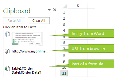
Tip: This clipboard is actually available in all of your Office programs.
Opening the Excel Clipboard
So where is this elusive clipboard you ask? All you need to do is click on the arrow in the Clipboard group on the home tab:
This will open the Clipboard pane to the left of the worksheet.
You can move, size and close it in the top right of the Clipboard pane:
Pasting from the Clipboard
To paste an item from the clipboard simply click on it, or hover your mouse over the item to reveal the down arrow where you can select ‘Paste’:
Deleting Items from the Clipboard
You can clear the entire Clipboard by clicking the ‘Clear All’ button* at the top, or click on the down arrow beside an item to delete items one by one:
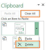
Note: *Clear All will clear all Clipboards since the Clipboard is actually shared amongst all of your Office programs.
Clipboard Settings
You can access the settings via the Options button at the bottom of the Clipboard:
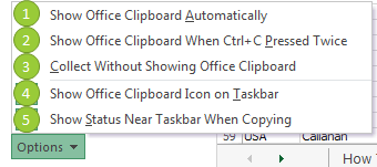
- Automatically displays the Office Clipboard when copying items.
- Automatically displays the Office Clipboard when you press CTRL+C twice.
- Automatically copies items to the Office Clipboard without displaying the Clipboard task pane.
- Displays the Office Clipboard icon in the status area of the system taskbar when the Office Clipboard is active. This option is turned on by default.
- Displays the collected item message when copying items to the Office Clipboard. This option is turned on by default but only displays when the Clipboard pane is open.

- Copying Formulas: Copying a cell containing a formula will copy the result as a value. If you want to copy the actual formula you must edit the cell (F2), then select the formula, or select it from the Formula bar and press CTRL+C to copy (see image below). You can press ESC to close the cell editing and the formula will still be available on the Clipboard.
Tip: You can copy parts of formulas you might want to reuse in other formulas and then paste them into your new formula as required.
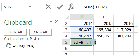
- Copying Formatted Text: If you want the formatting to remain when pasting make sure you copy the cell, as opposed to editing the cell and copying the text as per tip 1 above. In the image below you can see I’ve selected cell H6 and copied that to the Clipboard:
This will retain the red font formatting applied to ‘special’ when pasting from the Clipboard.
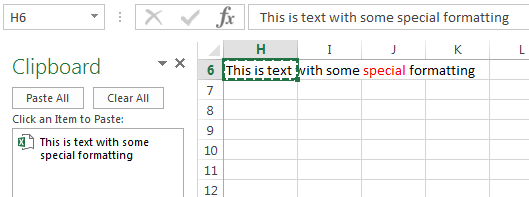
- Copying Values Only: If you don’t want to retain the formatting then edit the cell (F2) and select the text you want to copy and press CTRL+C to copy it to the Clipboard.
For a definitive guide on the Office Clipboard for all Office programs click here.