Copy and pasting cells in excel - Word и Excel - помощь в работе с программами

Move or copy cells and cell contents

Use Cut, Copy, and Paste to move or copy cell contents. Or copy specific contents or attributes from the cells. For example, copy the resulting value of a formula without copying the formula, or copy only the formula.

When you move or copy a cell, Excel moves or copies the cell, including formulas and their resulting values, cell formats, and comments.

You can move cells in Excel by drag and dropping or using the Cut and Paste commands.

Move cells by drag and dropping

Select the cells or range of cells that you want to move or copy.
Point to the border of the selection.
When the pointer becomes a move pointer , drag the cell or range of cells to another location.

Move cells by using Cut and Paste

Select a cell or a cell range.
Select Home > Cut or press Ctrl + X.
Select a cell where you want to move the data.
Select Home > Paste or press Ctrl + V.

Copy cells by using Copy and Paste

Select the cell or range of cells.
Select Copy or press Ctrl + C.
Select Paste or press Ctrl + V.

Need more help?

You can always ask an expert in the Excel Tech Community or get support in the Answers community.

Copy and Paste Multiple Adjacent Cells

Let’s start with the easy scenario.

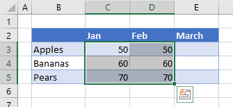
Suppose you have a range of cells (that are adjacent) as shown below and you want to copy it to some other location in the same worksheet or some other worksheet/workbook.

Below are the steps to do this:

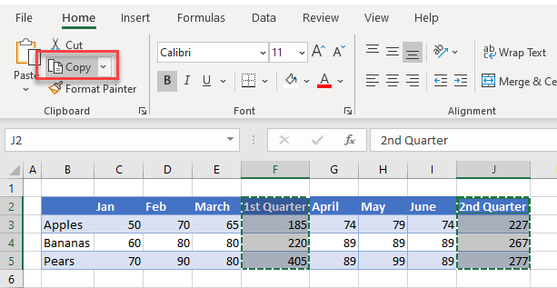
Select the range of cells that you want to copy

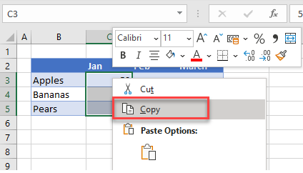
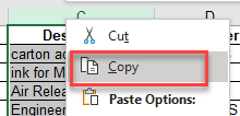
Right-click on the selection
Click on Copy

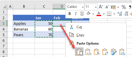
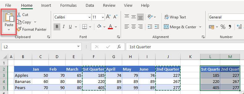
Right-click on the destination cell (E1 in this example)
Click on the Paste icon

Right click on destination cell and click on paste icon

The above steps would copy all the cells in the selected range and paste them into the destination range.

In case you already have something in the destination range, it would be overwritten.

Excel also gives you the flexibility to choose what you want to paste. For example, you can choose to only copy and paste the values, or the formatting, or the formulas, etc.

These options are available to you when you right-click on the destination cell (the icons below the paste special option).

Or you can click on the Paste Special option and then choose what you want to paste using the options in the dialog box.

Useful Keyboard Shortcuts for Copy Paste

In case you prefer using the keyboard while working with Excel, you can use the below shortcut:

Control + C (Windows) or Command + C (Mac) – to copy range of cells
Control + V (Windows) or Command + V (Mac) – to paste in the destination cells

And below are some advanced copy-paste shortcuts (using the paste special dialog box).

To use this, first copy the cells, then select the destination cell, and then use the below keyboard shortcuts.

To paste only the Values – Control + E + S + V + Enter
To paste only the Formulas – Control + E + S + F + Enter
To paste only the Formatting – Control + E + S + T + Enter
To paste only the Column Width – Control + E + S + W + Enter
To paste only the Comments and notes – Control + E + S + C + Enter

In case you’re using Mac, use Command instead of Control.

Also read: How to Cut a Cell Value in Excel (Keyboard Shortcuts)

Mouse Shortcut for Copy Paste

If you prefer using the mouse instead of the keyboard shortcuts, here is another way you can quickly copy and paste multiple cells in Excel.

Select the cells that you want to copy
Hold the Control key
Place the mouse cursor at the edge of the selection (you will notice that the cursor changes into an arrow with a plus sign)
Left-click and then drag the selection where you want the cells to be pasted

This method is also quite fast but is only useful in case you want to copy and paste the range of cells in the same worksheet somewhere nearby.

If the destination cell is a little far off, you’re better off using the keyboard shortcuts.

Copy and Paste Multiple Non-Adjacent Cells

Copy-pasting multiple cells that are nonadjacent is a bit tricky.

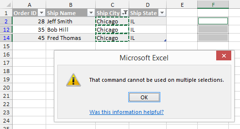
If you select multiple cells that are not adjacent to each other, and you copy these cells, you’ll see a prompt as shown below.

Excel doesnt allow copying non-adjacent cells

This is Excel’s way of telling you that you cannot copy multiple cells that are non-adjacent.

Unfortunately, there’s nothing that you can do about it.

There’s no hack or a workaround, and if you want to copy and paste these nonadjacent cells, you will have to do this one by one.

But there are a few scenarios where you can actually copy and paste non-adjacent cells in Excel.

Let’s have a look at these.

Copy and Paste Multiple Non-Adjacent Cells (that are in the same row/column)

While you can not copy non-adjacent cells in different rows and columns, if you have non-adjacent cells in the same row or column, Excel allows you to copy these.

For example, you can copy cells in the same row (even if these are non-adjacent). Just select the cells and then use Control + C (or Command + C for Mac). You will see the outline (the dancing ants outline).

Excel allows copying non-adjacent cells in the same row

Once you have copied these cells, go to the destination cell and paste these (Control + V or Command + V)

Excel will paste all the copied cells in the destination cell but make these adjacents.

Similarly, you can select multiple nonadjacent cells in one column, copy them, and then paste it into the destination cells.

Copy and Paste Multiple Non-Adjacent Rows/Columns (but adjacent cells)

Another thing Excel allows is to select non-adjacent rows or non-adjacent columns and then copy them.

Now when you paste these in the destination cell, these would be pasted as adjacent rows or columns.

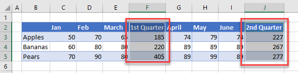
Below is an example where I copied multiple non-adjacent rows from the dataset and pasted these in a different location.

Copy Value From Above in Non-Adjacent Cells

One practical scenario where you may have to copy and paste multiple cells would be when you have gaps in a data set and you want to copy the value from the cell above.

Below I have some dates in column A, and there are some blank cells as well. I want to fill these blank cells with the date in the last filed cell above them.

To do this, I would need to do two things:

Select all the blank cells
Copy the date from the above-filled cell and paste it into these blank cells

Let me show you how to do this.

Select All Blank Cells in the Dataset

Below are the steps to select all the blank cells in column A:

Select the dates in column A, including the blank ones that you want to fill

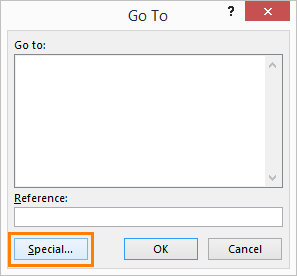
Press the F5 key on your keyboard. This will open the Go To dialog box.
Click the Special button. This will open the Go To Special dialog box.

In the Go To Special dialog box, select Blanks

Select Blanks in the Go To Special dialog box

Click OK

The above steps would select all the blank cells in column A.

Now, we want to somehow copy the value in the above field cell in these blank cells. This cannot be done using any copy-paste method so we will have to use a formula (a very simple one).

Fill Blank Cells with Value Above

This part is really easy.

With the blank cell selected, first hit the equal to key on your keyboard

Now hit the Up arrow key. This will automatically enter the cell reference of the cell that is above the active cell.

Hold the Control key and press the Enter key

The above steps would enter the same formula in all the selected blank cells – which is to refer to the cell above it.

Value from cell above is copied to the blank cells

While this is a formula, the end result is that you have the blank cells filled with the above-filled date in the data set.

Once you have the desired result, you can convert the formula into values if you want (so that the formula doesn’t update the cells in case you change any value in a cell that is being referenced in the formula).

So these are a couple of methods you can use to copy and paste multiple cells (adjacent and non-adjacent cells) in Excel. I am sure using these methods will help you save tons of time in your day-to-day work.

I hope you found this tutorial useful!

Other Excel tutorials you may also like:

How to Copy and Paste Column in Excel? 3 Easy Ways!
How to Copy Excel Table to MS Word (4 Easy Ways)
How to Copy Conditional Formatting to Another Cell in Excel
How to Copy and Paste Formulas in Excel without Changing Cell References
How to Edit Cells in Excel?

Источник

How to Copy and Paste in Excel – Step-By-Step (2023)

Copy/pasting is something we have all known for ages now. But there’s so much more to the dynamic copy-paste tool of Excel than simple copying/pasting of values.

And the guide below will show you how resourceful the copy-and-paste tool of Excel can be. So let’s dive right in👇

Hold on! Download our sample workbook here to tag along with the guide.

How to copy and paste into Excel

Unlike any other spreadsheet program, Excel offers a huge variety of options for copying/pasting data.

You can paste anything – formulas, formatting, values, transposed values, and whatnot🖌

And the best part is that you can access a single option from multiple places, offering extra ease of use. So how do you copy and paste values in Excel? Let’s see below

Generally, there are three 3️⃣ ways in which you can copy/paste your data once you select a cell.

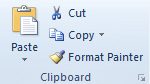
1. The clipboard group

The Clipboard section contains all the functions you need to copy and paste values in Excel. It sits in the Home tab of the ribbon.

The Paste function in Clipboard Section.

You can use the Scissors option to cut data and the Two Sheets option to copy the data✂

The Clipboard icon is the paste button that holds all the copied data. The Paint Brush icon below is known as the Format Painter, which lets you copy the formatting🖌

And the options don’t just end here – Click on the arrow in the bottom right corner to view more copy/paste options.

2. The right-click menu

You can access the context menu by right-clicking the cell you want to copy. The dropdown list will show you a bunch of options.

Choosing the Copy option from Context Menu.

Select Copy to make a copy of the selected cell in the clipboard. Once you copy a cell, a continuously moving border will enclose it.

Pro Tip!

You can also use CTRL + C to copy the data. It is the most common keyboard shortcut used in Excel and is very efficient.

Simply select the cell and press CTRL + C.

Then, select the destined cell and press CTRL + V to paste the copied contents into it 🥂

After you’ve copied the cell, navigate to the destination cell and paste it.

To paste the cell contents, right-click on the destination cell. From the context menu, select the option “Paste”📃

Choosing the Paste option from Context Menu.

3. The CTRL button

This method is quite similar to using CTRL + C, but not many people know it🤔

Select the cell.
Press the CTRL key.
Hover over the cell until the plus sign appears.
Hold and drag the cell to a new location.
You get an exact copy of your original cell in the new location.

How to copy formulas only in Excel

So now we know the basics of copy-pasting in Excel.

But do you know how to copy and paste only formulas in Excel? We do it using a trick.

Let’s see an example below.

The data set we use below shows if the given condition is true or false.

The function running behind these boolean values is the AND function. You can access it from the Formulas Tab 💻

Now let’s say we want to add another row at the bottom and copy the formula above it.

An easy way is to:

Copy the formula above by selecting any cell that contains the formula and press CTRL + C.
Right-click the cell where you want to paste the formula. A dropdown list will appear with the paste section like this ⏬

Click on the Paste Special commands option.
From the Paste Special menu, select the Formulas and Number formatting option (hovering over the icons shows their names).

The formula will be pasted into the new cell, and the cell references will adapt accordingly.

Similarly, if you want to copy the formula to multiple cells, you can do it using the Paste Special dialog box 💭

Launch the Paste Special Dialog box using the shortcut keys Alt + E + S.

Kasper Langmann, Microsoft Office Specialist

Simply select the Paste option you want to apply on the cell while pasting data. And since we are dealing with formulas, we will select the option “Formulas”.

How to make a copy of an Excel sheet

Making a copy of an Excel sheet may seem difficult with no options visible on the face of the worksheet. But believe us, it is just a click away.

Say, we want to make a copy of Sheet 1🧾

There are two ways to do this. First, use the right-click menu, and second, use the CTRL key.

The right-click context menu:

Select the sheet you want to copy.
Right-click the sheet and select the Move or Copy option.

You will see a pop-up asking for the location and whether you want to create a copy.

Check the option to Create a Copy.

What happens if you don’t check the option to create a copy🤔

Excel will remove the sheet from the present workbook. And move it to the destination workbook.

Kasper Langmann, Microsoft Office Specialist

Choose the pasting location from the To Book option.
Click Ok.

The subject worksheet appears in the chosen location💪

Using the CTRL key:

To copy a sheet using the Control key, follow the steps below:

Select the sheet.
Press the CTRL key.
Drag the sheet to a new location to make its copy.

We have created a copy of Sheet 1 in the same book.

A new file, Sheet 1 (2), appears on the Sheet tab.

Copy values not formula

It’s time we see how to copy only the values in Excel and not the underlying formulas.

From the dataset below, let’s copy the cell values only 🔢

To copy cell values, follow the steps below:

Select the cell or the range of cells whose value is to be copied.
Press Ctrl + C to copy the cell values.
Go to the blank cells where you want to paste the selected range.
Right-click the first cell and open the Paste Special dialog box.
From the Paste Special options, select the Values option.

This tells Excel to paste the values of the copied cells only 🌟

Click Okay. And there you go!

Values from the copied range appear in all the cells selected.

Note that Excel has pasted the exact values only. You can select the cell and view the formula bar to see that the values have no formulas to them.

Had you pasted them simply, Excel would have copied and adapted the formula of the copied cells for the destination cells as follows 😵

Shortcut to paste values

Oh, and there’s a very efficient shortcut to paste values in Excel too 💪

Select the values to be copied.
Press CTRL + C to copy them.
Go to the destination cells to paste values. Select the first cell of the destination cell range.
Press CTRL + Alt + V.
Press V.

Select Ok.
You’d have the cell values pasted in Excel without any cursor movement 🖱

How to copy formatting

We have so far seen how to copy and paste formulas and values. Let’s now have a look at the copy-pasting of formatting.

Hint: It’s done the same way as formulas and values are copied/pasted✌

We are using the same data set for this example. And we want to paste the existing formatting to the new cells below.

To do so:

Select the cells with the source formatting (the formatting that you want to copy) to copy them.
Once copied, select the cell (or cells) where you want to paste the cell formatting🖱
You can use the context menu to open the Paste Special dialog box and choose Formatting. Or press CTRL + Alt + V and then T to paste the formatting only.

The results look like this:

Note how Excel has pasted the format (including the font style and the font size) to the destined cells.

There is yet another way to copy cell formatting in Microsoft Excel – by using the Format Painter. We bet you didn’t see that coming😎

All you need to do is select the cells containing the source formatting. And click the Paintbrush icon on the ribbon to activate the Format Painter

Using the Format Painter to paste formatting.

With the format painter activated, select the cells where you want to paste the formatting.

And tada! The new cells are formatted like the source formatting.

Pro Tip!

If you want to paste the formatting to a single cell or a range of adjacent cells only, click on the format painter once. In this case, the format painter will deactivate after painting the format once.

But, if you want to apply the source formatting to multiple non-adjacent cells, double-press the Format Painter icon. Now the format painter will stay active until you manually deactivate it 🎨

That’s it – Now what?

In this article, we learned how to copy and paste values and formulas in Excel. We also saw how we could paste cell formatting to a range of cells in a few easy steps.

And even though this article covers most of the aspects of the copy-paste tool in Excel, there’s still so much to learn.

Like the three most important functions of Excel. The VLOOKUP, IF, and SUMIF functions.

To learn these functions (and more!), enroll in my 30-minute free email course today.

Kasper Langmann2023-01-19T12:05:51+00:00

Page load link

Источник

This tutorial demonstrates how to copy and paste multiple cells in Excel and Google Sheets.

Copy Adjacent Cells

Fill Handle

There are several ways that a range of cells can be copied and pasted in Excel. The simplest way to copy multiple or a range of cells across from one column or row to another is use the mouse to drag the values across from one column or row to the next.

In your worksheet, highlight the cells you wish to copy.

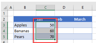
In the bottom-right corner of your selection, position your mouse so that the mouse pointer changes to a small cross.

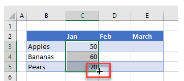
Drag the mouse across to the cells you wish to fill.

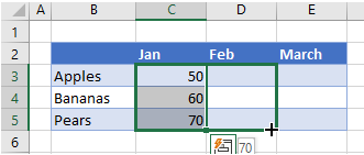
Release the mouse to copy the information into the blank cells.

‘

This method works well for both copying of cells from column across to an adjacent column on the right, or from a row down to the next row.

Quick Menu

In your worksheet, highlight the cells you wish to copy.

Right-click on the cells you wish to copy to view the quick menu and click Copy.

Note that the source cells have small moving lines around them indicating that the information is ready to paste.

Select the first destination cell and then right-click once again and click Paste.
OR Press the ENTER key on the keyboard to paste the cell data.
Note: You do not have to select the entire destination range where you wish to paste the cell information; you only need to select the first cell.

Copy Nonadjacent Cells

In your worksheet, highlight the nonadjacent cells you wish to copy by highlighting the first range of cells, and then holding down the CTRL key, highlight the second range of cells.

Then, in the Ribbon, go to Home > Clipboard > Copy or press CTRL + C on the keyboard. Notice that small little moving lines appear around both selected ranges.

Select the cell where you wish to paste your data and then, in the Ribbon, go to Home > Clipboard > Paste (or press CTRL + V on the keyboard).

When you click Paste on the Ribbon, or type CTRL + V on the keyboard, you are left with the small moving lines around your original cells. This is because the information is still on the clipboard and can be pasted as often as you like by using CTRL + V or clicking Paste in the Ribbon. If you wish to exit this mode you can either use ENTER on the keyboard to paste your data, or, if you have already pasted your data, you can press ESC on the keyboard to remove the small moving lines.

Copy Entire Columns and/or Rows

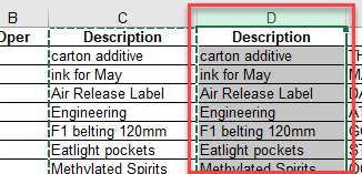
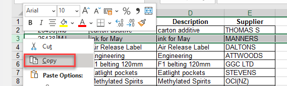
To copy a column, select the entire column using the column header.

Right-click to bring up the quick menu and click Copy.

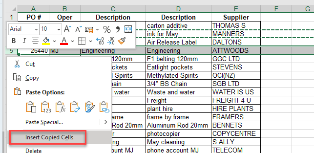
Select the column where you want to paste the copied cells, and right-click on the column header of the destination column. Click Insert Copied Cells.

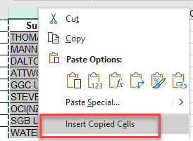
A new column is inserted before the column you selected. This new column will contain the copied cells.

Note: if you have selected a blank column (i.e., no data in any of the cells), you can just press ENTER on the keyboard or choose Paste from the quick menu to paste the copied data into the existing column.

You copy a row in the same way.

Click in the row header of the row you wish to copy to select the row, and then right-click and click Copy.

Right-click on the destination row header and to insert a row with the copied data, click Insert Copied Cells, or click Paste to paste the data into an existing row.

Copy Formulas

If you have a cell with a formula in it, and you wish to use that formula in adjacent, or nonadjacent cells, you can copy the formula in the same way as you would copy cells above.

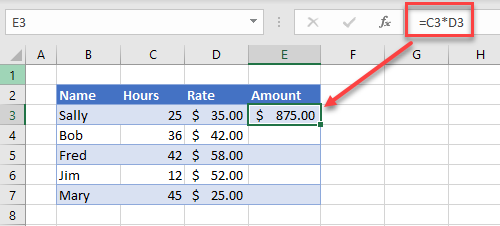
Select the cell that contains the formula, and then either:
Right-click, and then click Copy.
OR Press CTRL + C on the keyboard.
OR In the Ribbon, go to Home > Clipboard > Copy.

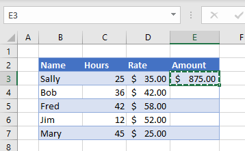
Small moving lines indicate that the cell has been copied.

Select the cells where you want to paste the formula.

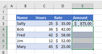
Right-click, and then click Paste.
OR Press CTRL + V or ENTER on the keyboard.
OR In the Ribbon, go to Home > Clipboard > Paste.

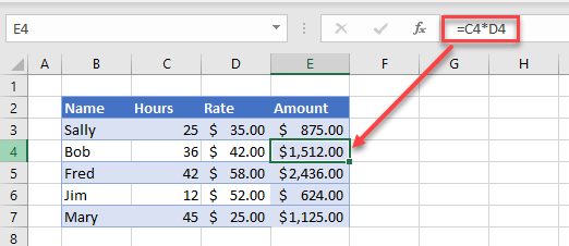
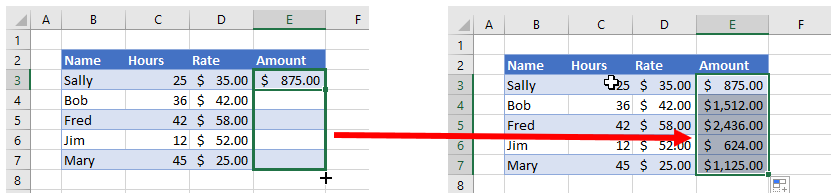
As you look down at the copied formula, you will notice that the formula automatically changes according to the row and column you are copying down or across to.

Note: You can also copy and paste an exact formula so that the row and column information don’t change.

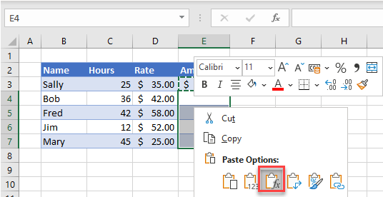
Copy Cell Data or Formula

In the picture above, the formatting from cell E3 was pasted into cells E4:E7 along with the formula. The same thing happens when you copy cell data without a formula. To prevent this from happening, use Paste Options to just paste the formulas without the format.

Copy the cell.
Then, right-click and choose Paste Options > Paste Formulas.

OR
In the Ribbon, go to Home > Clipboard > Paste > Paste Formulas.

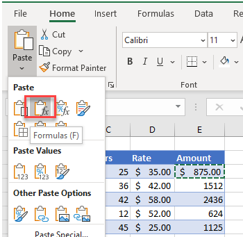
This pastes the formulas into the selected cells without any formatting.

Copy a Formula to Adjacent Cells

You can also drag the formula down to the adjacent cells by using the fill handle.

Notes

Note that this method will also copy the formatting down to the adjacent cells along with the formula.
It’s also possible to use Paste Options to paste the formula as text.

Copy-Paste Multiple Cells in Google Sheets

Copying and pasting in Google Sheets works in much the same way as it does in Excel.

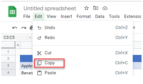
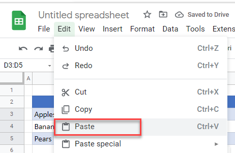
Highlight the cells you wish to copy, and then, on the keyboard press CTRL + C or in the Menu, go to Edit > Copy.

Select the destination cell and press CTRL + V on the keyboard, or in the Menu, go to Edit > Paste.

You may get a message that you need to install an extension to use Edit > Paste.

You can either dismiss the information message and use CTRL + V to paste the cell data, or you can install the extension into your browser to enable you to use Edit > Paste on the menu.
As with Excel, you can use Paste Special to paste only part of the cell contents: formulas, values, format, etc.

In the Menu, go to Edit > Paste special and then select the option required.

Adjacent Cells

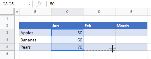
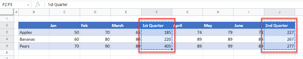
To copy the cell data across to adjacent cells using the mouse, highlight the cells containing the data, and then, drag the mouse pointer across to the desired destination cells.

Nonadjacent Cells

Selecting nonadjacent cell ranges in Google Sheets works the same as in Excel. Select the first range then, holding down the CTRL key, select the second range. Then copy both ranges using CTRL + C or in the Menu, go to Edit > Copy.

Select the destination location and the press CTRL + V or, in the Menu, go to Edit > Paste.

Copy Entire Columns and Rows

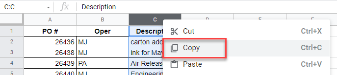
As with Excel, right-click in the header of the column, then click Copy.

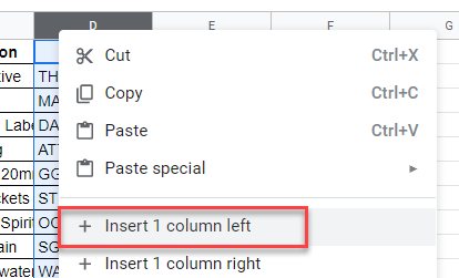
Right-click in the column header of the destination column. Google will not automatically insert a new column so insert a column first if you do not wish to overwrite the data already in the column. Click Insert 1 column left.

Right-click in the new column header and click Paste.

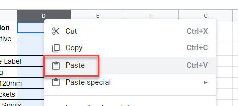
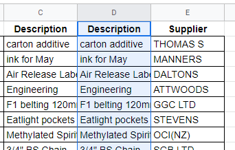
The copied data is pasted into the new column.

Copying an entire row works in the same way; just click the row header instead of the column header!

More Options

For more information on copying and pasting in Excel and Google Sheets, see:

Copy and Paste Exact Formula
Copy and Paste Non-Blank Cells (Skip Blanks)
Copy and Paste Without Borders
Paste Horizontal Data Vertically
Rearrange Columns
Duplicate Rows
VBA Value Paste & Paste Special
VBA – Cut, Copy, Paste from a Macro
VBA Copy / Paste Rows & Columns
Select Nonadjacent Cells or Columns
Copy Cell From Another Sheet

Источник

Working in spreadsheets all day? Check out these 15 copy & paste tricks to save time when you’re copying and pasting cells in Microsoft Excel.

Excel is one of the most intuitive spreadsheet applications to use. But when it comes to copying and pasting data throughout different parts of the spreadsheet, most users don’t realize how many possibilities there are.

Whether you want to copy and paste individual cells, rows or columns, or entire sheets, the following 15 tricks will help you do it faster and more efficiently.

1. Copy Formula Results

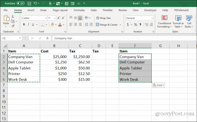
One of the most annoying things about copying and pasting in Excel is when you try to copy and paste the results of Excel formulas. This is because, when you paste formula results, the formula automatically updates relative to the cell you’re pasting it into.

You can prevent this from happening and copy only the actual values using a simple trick.

Select the cells with the values you want to copy. Right-click any of the cells and select Copy from the pop-up menu.

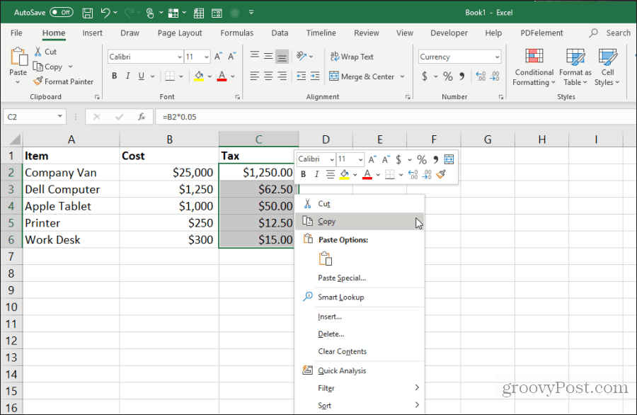
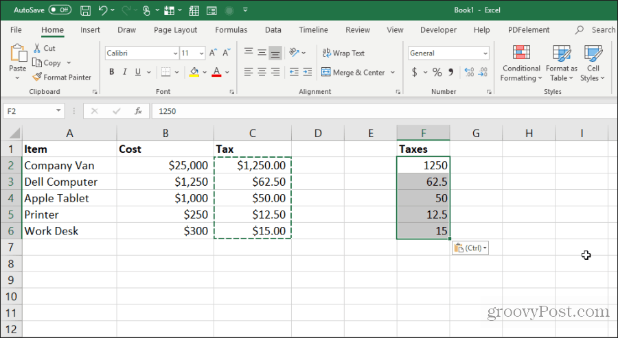
Right-click the first cell in the range where you want to paste the values. Select the Values icon from the pop-up menu.

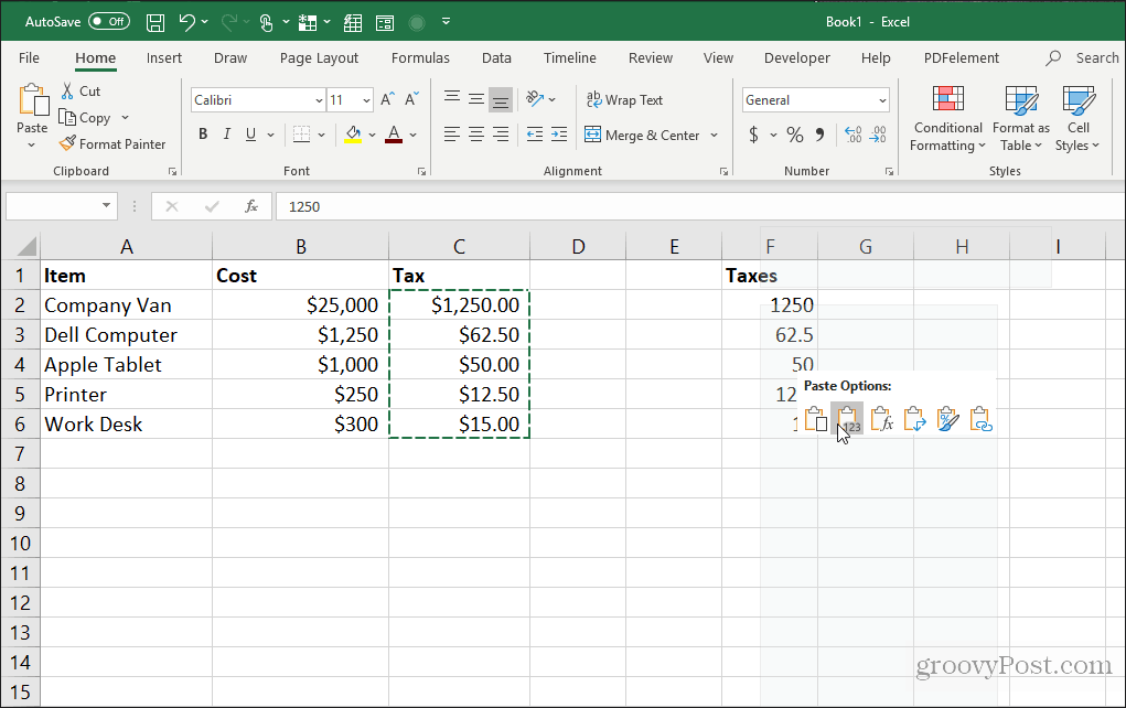
This will paste only the values (not the formulas) into the destination cells.

This removes all of the relative formula complexity when you normally copy and paste formula cells in Excel.

2. Copy Formulas Without Changing References

If you want to copy and paste formula cells but keep the formulas, you can do this as well. The only problem with strictly pasting formulas is that Excel will automatically update all the referenced cells relative to where you’re pasting them.

You can paste the formula cells but keep the original referenced cells in those formulas by following the trick below.

Highlight all of the cells that contain the formulas you want to copy. Select the Home menu, click on the Find & Select icon in the Editing group, and select Replace.

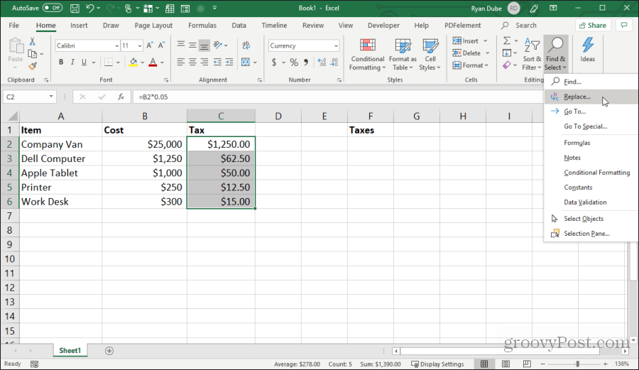
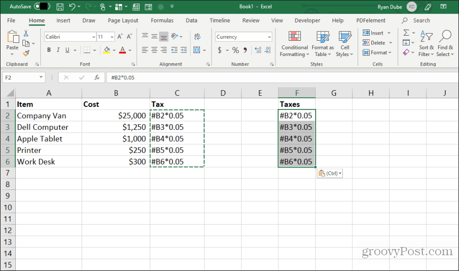
In the Find and Replace window, type = in the Find what field, and # in the Replace with field. Select Replace All. Select Close.

This will convert all formulas to text with the # sign at the front. Copy all of these cells and paste them into the cells where you want to paste them.

Next, highlight all of the cells in both columns. Hold down the Shift key and highlight all cells in one column. Then hold down the Control key and select all of the cells in the pasted column.

With all cells still highlighted, repeat the search and replace procedure above. This time, type # in the Find what field, and = in the Replace with field. Select Replace All. Select Close.

Once the copy and replace are done, both ranges will contain the same formulas without shifting references.

This procedure may seem like a few extra steps, but it’s the easiest to override the updated references in copied formulas.

3. Avoid Copying Hidden Cells

Another common annoyance when copying and pasting in Excel is when hidden cells get in the way when you copy and paste. If you select and paste those cells, you’ll see the hidden cell appear in the range where you paste them.

If you only want to copy and paste the visible cells, select the cells. Then in the Home menu, select Find & Select, and then select Go To Special from the dropdown menu.

In the Go To Special window, enable Visible cells only. Select OK.

Now press Control+C to copy the cells. Click on the first cell where you want to paste, and press Control+V.

This will paste only the visible cells.

Note: Pasting the cells into a column where an entire second row is hidden will actually hide the second visible cell you’ve pasted.

4. Fill to Bottom with Formula

If you’ve entered a formula into a top cell next to a range of cells already filled out, there’s an easy way to paste the same formula into the rest of the cells.

The typical way people do this is to click and hold the handle on the bottom left of the first cell and drag it to the bottom of the range. This will fill in all cells and update cell references in the formulas accordingly.

But if you have thousands of rows, dragging all the way to the bottom can be difficult.

Instead, select the first cell, then hold down the Shift key and hover the house over the lower-right handle on the first cell until you see two parallel lines appear.

Double click on this double-line handle to fill to the bottom of the column with data to the left.

This technique to fill cells down is fast and easy and saves a lot of time when you’re dealing with extensive spreadsheets.

5. Copy Using Drag and Drop

Another neat time-saver is copying a group of cells by dragging and dropping them across the sheet. Many users don’t realize that you can move cells or ranges just by clicking and dragging.

Give this a try by highlighting a group of cells. Then hover the mouse pointer over the edge of the selected cells until it changes to a crosshair.

Left-click and hold the mouse to drag the cells to their new location.

This technique performs the same action as using Control-C and Control-V to cut and paste cells. It’ll save you a few keystrokes.

6. Copy from Cell Above

Another quick trick to save keystrokes is the Control+D command. If you place the cursor under the cell, you want to copy, press Control+D, and the cell above will get copied and pasted into the cell you’ve selected.

Control+Shift+’ performs the same action as well.

7. Copy from Left Cell

If you want to do the same thing but copying from the cell to the left instead, select the cell to the right and press Control+R.

This will copy the cell to the left and paste it in the cell to the right, with just one keystroke!

8. Copy Cell Formatting

Sometimes, you may want to use the same formatting in other cells that you’ve used in an original cell. However, you don’t want to copy the contents.

You can copy just the formatting of a cell by selecting the cell, then type Control+C to copy.

Select the cells you want to format like the original, right-click, and select the formatting icon.

This will paste only the original formatting but not the content.

9. Copy Entire Sheet

If you’ve ever wanted to work with a spreadsheet but didn’t want to mess up the original sheet, copying the sheet is the best approach.

Doing this is easy. Don’t bother to right-click and select Move or Copy. Save a few keystrokes by holding down the Control key, left-click on the sheet tab, and dragging it to the right or the left.

You’ll see a small sheet icon appear with a + symbol. Release the mouse button, and the sheet will copy where you’ve placed the mouse pointer.

10. Repeat Fill

If you have a series of cells that you want to drag down a column and have those cells repeat, doing so is simple.

Just highlight the cells that you want to repeat. Hold down the Control key, left-click the lower right corner of the bottom cell, and drag down the number of cells that you’d like to repeat.

This will fill all of the cells below the copied ones in a repeating pattern.

11. Paste Entire Blank Column or Row

Another trick to save keystrokes is adding blank columns or rows.

The typical method users use to do this is right-clicking the row or column where they want a blank and selecting Insert from the menu.

A faster way is to highlight the cells that make up the row or column of data where you need the blank.

Holding down the Shift key, left-click the bottom right corner of the selection, and drag down (or to the right if you selected a column range).

Release the mouse key before you release Shift.

This will insert blanks.

12. Paste Multiples of a Single Cell

If you have a single cell of data that you want to replicate over many cells, you can copy the individual cell and paste it over as many cells as you like. Select the cell you want to copy and press Control+C to copy.

Then choose any range of cells where you want to copy the data.

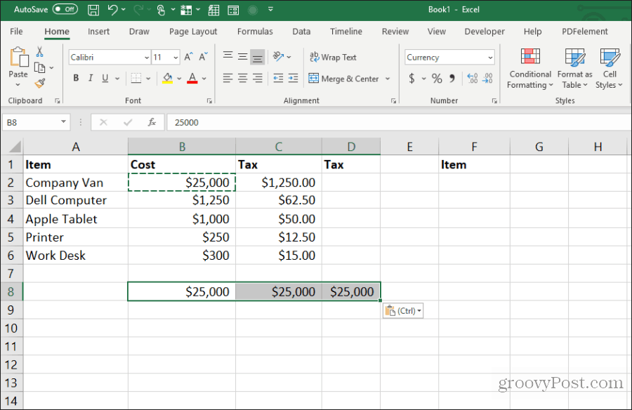
This will replicate that cell across as many cells as you like.

13. Copy Column Width

When copying and pasting a column of cells and you want the destination to be the same width as the original, there’s a trick to that as well.

Just copy the original column of cells as you normally would using the Control-C keys. Right-click the first cell in the destination and press Control-V to paste.

Now, select the original column of cells again and press Control-C. Right-click the first cell in the column you previously pasted and choose Paste Special.

In the Paste Special window, enable Column widths and select OK.

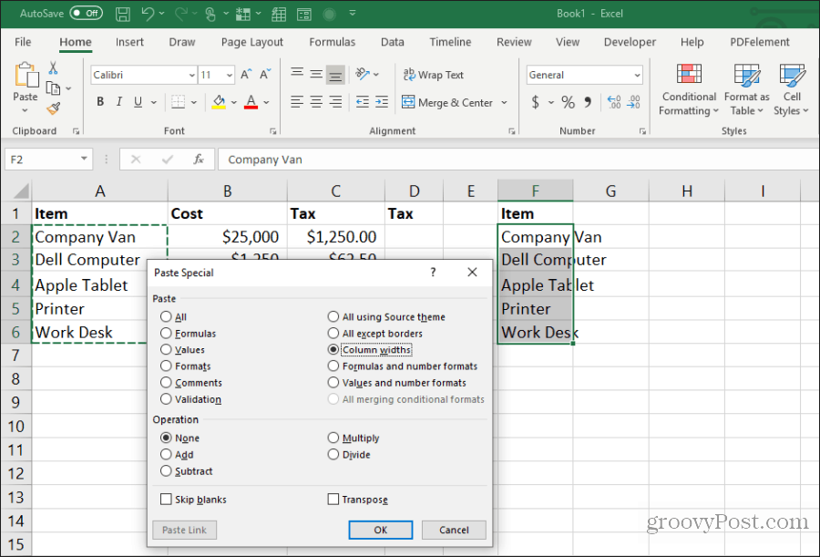
This will automatically adjust the column width to match the original widths as well.

It might be easier to adjust the column width with your mouse, but if you’re adjusting the width of multiple columns at once on a huge sheet, this trick will save you a lot of time.

14. Paste with Calculation

Have you ever wanted to copy a number to a new cell but perform a calculation on it simultaneously? Most people will copy the number to a new cell and then type a formula to perform the calculation.

You can save that extra step by performing the calculation during the paste process.

Starting with a sheet containing the numbers you want to calculate, first select all of the original cells and press Control+C to copy. Paste those cells into the destination column where you want the results.

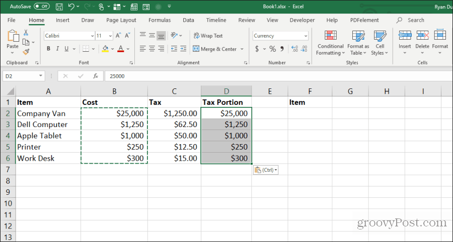
Next, select the second range of cells you want to calculate and press Control+C to copy. Select the destination range again, right-click, and choose Paste Special.

In the Paste Special window, under Operation, select the operation you want to perform on the two numbers. Select OK, and the results will appear in the destination cells.

This is a fast and easy way to perform quick calculations in a spreadsheet without using extra cells to do quick calculations.

15. Transpose Column to Row

The most useful paste trick of all is transposing a column into a row. This is especially useful when you have one sheet with items vertically along a column that you want to use as headers in a new sheet.

First, highlight and copy (using Control+C) the column of cells you want to transpose as a row in your new sheet.

Switch to a new sheet and select the first cell. Right-click and select the transpose icon under Paste Options.

This pastes the original column into the new sheet as a row.

It’s fast and easy and saves the trouble of copying and pasting all of the individual cells.

Use all of the 15 tips and tricks above to save yourself a lot of time the next time you’re working with your Excel worksheets.

Источник

Learn how to copy and paste excluding hidden columns or rows in Excel.

Ever tried to copy and paste data thinking you will be pasting, excluding the hidden columns or rows only to have the hidden data copied too?

Copying a data range that contains hidden data can be challenging when the hidden data travels with the copied range.

In this post I’ll explain how to copy and paste the visible cells only – hidden cells are excluded.

This blog includes step-by-step help on the following:

Why does Copy and Paste include hidden data in Excel?
Copying and pasting visible cells only in Excel (excluding hidden cells)
Excel Shortcuts for Copying and Pasting visible cells only (excluding hidden cells)

Why does Copy and Paste include hidden data in Excel?

Let’s look at what happens when we try to copy and paste a range with hidden data. In the example below we have an Excel spreadsheet with information on sales.

Excel Sales spreadsheet with information on sales made over the past year. Information includes Invoice # (Column A), Date (Column B), Customer Name (Column C), Product Name (Column D), Product Type (Column E), UOM (Column F), Cost Price (Column G), RRP (Column H), Sales Price (Column I), Quantity sold (Column J), Total Sales $ (Column K and Salesperson (Column L).

In this example, we are wanting to hide rows 6-9 and copy and paste the information in this data set without these rows included.

To follow along, rows 6-9 have been highlighted in yellow so that they are easily identified as we continue through the steps.

Excel Sales spreadsheet with columns 6-9 highlighted in yellow

To hide these rows, we will do the following.

Step 1: Select the rows we want hidden by clicking and dragging over the row numbers. In our example, this is rows 6-9.

Excel Sales spreadsheet with rows 6-9 highlighted and selected

Step 2: Right-click the selected rows and then select Hide from the menu.

List from right clicking with multiple options and mouse hovering over the Hide option

The rows we have selected will now be hidden.

You can see in our example, rows 6-9 are hidden. We can easily identify this as the highlighted rows are now hidden and the row numbers jump from 5 to 10.

Excel Sales spreadsheet with rows 6-9 hidden and a red box on the row tabs showing that they are hidden

Copying data that has hidden rows

Now let’s try copying the first 3 columns of data in this table to another worksheet. We are assuming that the hidden data will not copy because it is hidden.

Step 1: We will select the data range that we want to copy, including the hidden rows. In this example, we want to copy the Invoice number, Date and Customer Name columns.

Sales spreadsheet with columns Invoice # (Column A), Date (Column B) and Customer Name (Column C) are selected

Step 2: To copy the range we’ve selected, we will right-click the selected range and select Copy from the shortcut menu (or press Ctrl + C).

Shortcut menu with the mouse hovering over the Copy option

Step 3: We will now go to where we want to paste the data and select the cell that will be the top, left cell of the pasted range. In our example, we created a new sheet and are now wanting to paste the copied data into cell A3. The name of our new sheet is Sheet1 as this was the default name given to the sheet by Excel.

Sheet1 in the workbook with cell A3 selected

Step 4: We will now paste the copied data by doing a right-click and selecting Paste from the shortcut menu (or we can press Ctrl + V).

Shortcut menu with the mouse hovering over the paste option

Step 5: Unfortunately, we can see that the hidden data has been copied and included when we paste. This is easily identifiable as you can see the rows we highlighted in yellow, prior to doing the copy, have also copied over.

Sheet1 with pasted information and rows 6-9 are highlighted in yellow

This is because when we selected the data to be copied in Step 1, we are actually selecting both visible AND hidden data.

Therefore, when we copied we are copied ALL the data, not just the visible cells.

Most of the time this is not ideal, and you don’t want these hidden rows to travel over with the data you are copying and pasting.

The following steps will teach you how to paste visible cells only in Excel, excluding any hidden rows or columns.

Copying and pasting visible cells only in Excel (excluding hidden cells)

Step 1: Start by selecting the area you want to copy. In our example we will select the Invoice, Date and Customer Name columns. The highlighted rows 6 to 9 are hidden.

Sales spreadsheet with columns Invoice # (column A), Sale (Column B) and Customer Name (Column C) all highlighted

Step 2: From the Home tab, select Find & Select.

Home tab in Excel with a red box showing where Find & Select is

Step 3: Select Go To Special.

Find & Select is selected with the mouse hovering over the Go To Special option

The Go To Special dialogue box will appear.

Go To Special Dialogue box with Notes selected

Step 4: Select Visible cells only. This ensures only the visible cells are included in your selection. The hidden cells are excluded.

Go To Special dialogue box with Visible cells only selected

Step 5: Click OK.

Go To Special dialogue box with Visible cells only selected and the mouse over OK

You will now see that the visible cells have been selected and the hidden cells are excluded. A small line within the selected area shows this .

A red box showing where there is a small line indicating that there are rows hidden in this area. The line is between rows 5 and 10

Step 6: Now Copy the selected cells by right-clicking over the selected area and selecting Copy from the shortcut menu (or press Ctrl + C).

Columns A B and C are selected with shortcut menu and mouse over the option Copy

Step 7: Go to where you want to paste the data and select the cell that will be the top, left cell of the pasted range. In our example, we created a new sheet called Sheet 1 as this is the default name given by Excel and we selected cell A3.

Sheet1 with cell A3 selected

Step 8:
Paste by doing a right-click and selecting Paste from the shortcut menu (or press Ctrl + V).

Shortcut menu with the mouse over the Paste option

Super Tip: If you want to paste your cells with the exact same column widths as the sheet they were copied from, when you go to paste do a right-click and select Paste Special. From there, select Keep Source Column Widths (W).

Only the visible cells will be pasted.

In this example, we can easily tell that only the visible cells have been pasted as the hidden rows were highlighted in yellow and they have not appeared.

Sheet1 in the workbook with Invoice # information starting in cell A3, Date information starting in cell B3 and Customer Name information starting in tow C3

Excel Shortcuts for Copying and Pasting visible cells only (excluding hidden cells)

1. Select the range to be copied, including the hidden data.

2. Press ALT + ; (ALT + semicolon to select only visible data and exclude any hidden data)

3. Press Ctrl + C (to copy)

4. Go to where you want to paste the data and select the cell that will be the top, left cell of the pasted range.

5. Press Ctrl + V (to paste the data).

To Sum up

The trick is to ensure you are only selecting visible cells prior to doing your Copy.

Once you have this mastered you can easily control your data and copy visible cells only.

Was this blog helpful? We’d love to know. If you’re a beginner or if you use Excel every day please let us know if we helped in some way by leaving a Comment below.

Instructions

Copying and pasting visible cells only in Excel (excluding hidden cells)

Select the area you want to copy.
From the Home tab, select Find & Select.
Select Go To Special. The Go To Special dialogue box will appear.
Select Visible cells only. This ensures only the visible cells are included in your selection. The hidden cells are excluded.
Click OK. You will now see that the visible cells have been selected and the hidden cells are excluded. A small line within the selected area shows this.
Now Copy the selected cells by right-clicking over the selected area and selecting Copy from the shortcut menu (or press Ctrl + C).
Go to where you want to paste the data and select the cell that will be the top, left cell of the pasted range.
Paste by doing a right-click and selecting Paste from the shortcut menu (or press Ctrl + V).

Excel Shortcuts for Copying and Pasting visible cells only (excluding hidden cells)

Select the range to be copied, including the hidden data.
Press ALT + ; (ALT + semicolon to select only visible data and exclude any hidden data)
Press Ctrl + C (to copy)
Go to where you want to paste the data and select the cell that will be the top, left cell of the pasted range.
Press Ctrl + V (to paste the data).

Notes

Why does Copy and Paste include hidden data in Excel?

When you select a range that has hidden data, you are also selecting that hidden data. This means that when you copy and paste the data, the hidden data will be copied and pasted with it. If you want to copy and paste visible cells only, the trick is to ensure you are only selecting visible cells prior to doing your Copy.

Copying and pasting visible cells only in Excel (excluding hidden cells)

If you enjoyed this post check out the related posts below.

Elevate your Excel game and become a pro with our exclusive Insider Group.

Be the first to know about new tutorials, videos, and tips for Microsoft 365 products. Join us now and claim your exclusive bonus today!

Источник

Copying and pasting is a very frequently performed action when working on a computer. This is also true in Excel.

It’s so common that almost everyone knows the keyboard shortcuts to copy Ctrl + C and paste Ctrl + V.

When using this in Excel, it will copy everything including values, formulas, formatting, comments/notes, and data validation.

This can be frustrating as sometimes you’ll only want the values to copy and not any of the other stuff in the cells.

In this post, you’ll learn all the ways to copy and paste only the values from your Excel data.

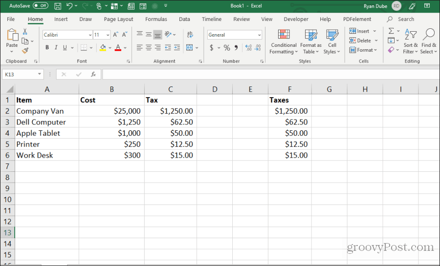
Example Data

The example data used in this post contains various formatting.

Cell formatting such as font color, fill color, number formatting, and borders.
Notes.
SUM formula.
A data validation dropdown list.

Paste Special Keyboard Shortcut

If you want to copy and paste anything other than an exact copy, then you’re going to need to become familiar with paste special.

A favorite method to use this is with a keyboard shortcut.

To use the paste special keyboard shortcut.

Copy the data you want to paste as values into your clipboard.
Choose a new location in your workbook to paste the values into.
Press Ctrl + Alt + V on your keyboard to open up the Paste Special menu.
Select Values from the Paste option or press V on your keyboard.
Press the OK button.

This will paste your data without any formatting, formulas, comments/notes, or data validation. Nothing but the values will be there.

Paste Special Legacy Keyboard Shortcut

This keyboard shortcut is a legacy shortcut from before the Excel ribbon command existed and it’s still usable.

In fact, when you try and use this you’ll be greeted with the above warning to let you know this is from an earlier version of Microsoft Office.

When you have a range of data copied to your clipboard, you can open up the Paste Special menu by pressing Alt + E + S on your keyboard.

Once the Paste Special menu is open you can then press V for Values.

One advantage the legacy shortcut has is it can easily be performed with one hand!

Paste Special Values Keyboard Shortcut

Pasting as values is a very common activity in Excel. Because of this, a new keyboard shortcut was introduced to Microsoft 365 users for this exact purpose.

Press Ctrl + Shift + V on your keyboard to paste the last item in your clipboard as values.

This is the most useful new shortcut as it bypasses the paste special menu entirely.

Paste Special from the Home Tab

If you’re not a keyboard person and prefer using the mouse, then you can access the Paste Values command from the ribbon commands.

Here’s how to use Paste Values from the ribbon.

Select and copy the data you want to paste into your clipboard.
Select the cell you want to copy the values into.
Go to the Home tab.
Click on the lower part of the Paste button in the clipboard section.
Select the Values clipboard icon from the paste options.

The cool thing about this menu is before you click on any of the commands you will see a preview of the data you’re about to paste. This makes it easy to ensure you’re selecting the right option.

Paste Values with Hotkey Shortcuts

Since the paste values command is in the ribbon, that also means you can access it with the Alt hotkeys.

Notice when you press the Alt key, the ribbon lights up with all the accelerator keys available.

Pressing Alt ➜ H ➜ V ➜ V will activate the paste values command.

Paste Values from Right Click Menu

Paste Values is also available from the right-click menu.

Copy the range of cells you want to paste as values ➜ right click ➜ select the paste values clipboard icon.

Paste Values with Quick Access Toolbar Command

If it’s a command you use quite frequently, then why not put it in the quick access toolbar?

This way it’s only a click away at all times!

Depending on where in the quick access toolbar you place it, it will also get its own easy to use Alt hotkey shortcut too.

Check out this post for details on how to add commands to the quick access toolbar, or this post on other interesting commands you can add to the quick access toolbar.

You can add the paste values command from the Excel Options screen.

Select All Commands from the dropdown list.
Locate and select Paste Values from the options. You can press P on your keyboard to quickly navigate to commands starting with P.
Press the Add button.
Use the Up and Down arrows to change the ordering of commands in your toolbar.
Press the OK button.

The command will now be in your quick access toolbar!

If you place it in the 4th position like in this Example, then you can you Alt + 4 to access it with a keyboard shortcut.

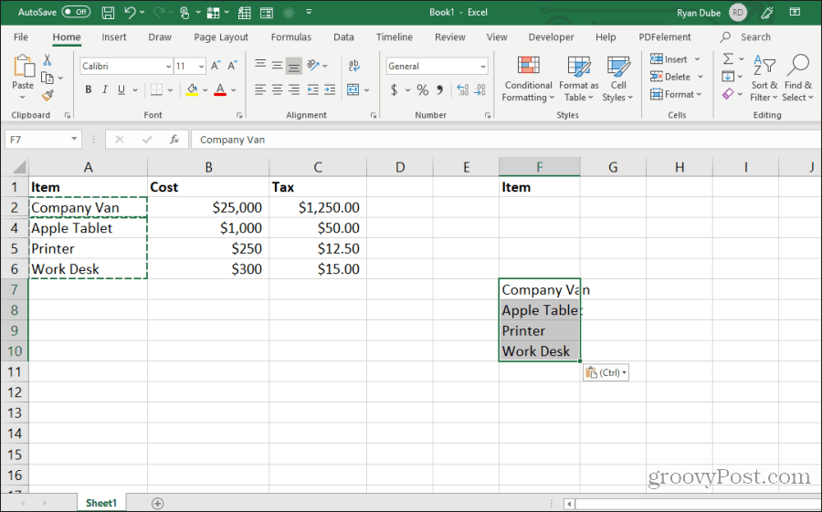
Paste Values Mouse Trick

There’s a mouse option you can use to copy as values which most people don’t know about.

Select the range of cells to copy.
Hover the mouse over the active range border until the cursor turns into a four directional arrow.
Right-click and drag the range to a new location.
When you release the right click, a menu will pop up.
Select Copy Here as Values Only from the menu.

This is such a neat way, and there are a few other options in this hidden menu that are worth exploring.

Paste Values with Paste Options

There’s another sneaky method to paste values.

When you do a regular copy and paste, a small icon will appear in the bottom right corner of the pasted range. It will remain there until you interact with something else in your spreadsheet.

These are the paste options and you can click on it or press Ctrl to expand the options menu.

When you open the menu, you can then either click on the Values icon or press V to change the range into values only.

Paste Values and Formulas with Text to Columns

I don’t really recommend using this method, but I’m going to add it just for fun.

A few caveats with this method.

You can only copy and paste one column of data.
It will keep any formulas.
It will remove the formatting, comments, notes, and data validation.

If that’s exactly what you’re looking for, then this method might be of interest.

Select a single column of data ➜ go to the Data tab ➜ select the Text to Column command.

This will open up the Convert Text to Column Wizard. In the first step, you can select Delimited and press the Next button.

You can also select Fixed width as we won’t be using the text to column functionality it doesn’t really matter.

In the next step, remove any selected delimiters and press the Next button.

In the last step, select the destination cell for the output and press the Finish button.

You can see the results have all the formatting gone but any formulas still remain.

Paste Values with Advanced Filters

This one is another not-quite paste values option and is listed for fun as well.

It will remove any formulas, comments, notes, and data validation but will leave all cell formatting.

With your data selected go to the Data tab then select the Advanced command in the Sort and Filter section.

From the Advanced Filter Menu.

Select Copy to another location.
Leave the Criteria range empty.
Select a location to place the copied data.
Press the OK button.

This will create a copy of the data as values and remove any formulas, comments, notes, and data validation.

You can then remove the cell formatting that’s left by going to the Home tab ➜ Clear ➜ and selecting the Clear Formats option.

Conclusions

Wow! That’s a lot of different ways to paste data as values in Excel.

It’s understandable there are so many options given it’s an essential action to avoid carrying over unwanted formatting.

You’re eventually going to need to do this and there are quite a few ways to get this done.

What’s your favorite way? Did I miss any methods you use? Let me know in the comments!

About the Author

John MacDougall

John is a Microsoft MVP and qualified actuary with over 15 years of experience. He has worked in a variety of industries, including insurance, ad tech, and most recently Power Platform consulting. He is a keen problem solver and has a passion for using technology to make businesses more efficient.

Источник

Have you ever tried to copy and paste a range with hidden rows or columns and didn’t get the results you expected? This problem can be frustrating and time consuming! In this post and video I will explain how to solve this problem with a very simple shortcut to select the visible cells only.

Have you ever tried to copy and paste a range with hidden rows or columns and didn’t get the results you expected?

This problem can be frustrating and time consuming! In this post and video I will explain how to solve this problem with a very simple shortcut. The shortcut will select the visible cells only in a range, ignoring the hidden rows and columns.

Please leave a comment below with any questions.

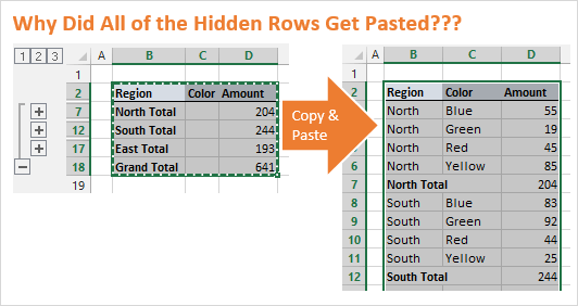
Why Are My Hidden Rows & Columns Being Pasted?

When you copy a range of cells that contains hidden rows or columns, Excel includes ALL of the selected rows. It does not matter if they are visible or hidden. When you go to paste the range, all the cells in the selection will be pasted.

This is actually a nice feature, but it’s not always what we are expecting to happen. Sometimes we only want to copy and paste the visible cells, and exclude the hidden rows & columns.

This commonly happens when you are working with a range that has filters applied to it. Or when you have hidden rows or columns from a collapsed group in an outline. The Subtotals feature automatically creates row groupings that can cause rows to be hidden, as shown in the example above.

Select the Visible Cells Only

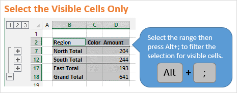
Excel gives us an option to select the visible cells only using the keyboard shortcut Alt+; (hold down the Alt key, then press the semi-colon key). The Mac shortcut is Cmd+Shift+Z.

This shortcut will exclude all the hidden rows and columns from the selection.

Copy & Paste Visible Cells

Here are instructions on how to copy and paste visible cells only (please see the video above for details):

Select the entire range you want to copy.
Press Alt+; to select the visible cells only. You will notice that the selection is cut up to skip the hidden rows and columns.
Copy the range – Press Ctrl+C or Right-click>Copy
Select the cell or range that you want to paste to
Paste the range – Press Ctrl+V or Right-click>Paste

Alternatives to Alt+;

If you don’t use this shortcut often then it might be hard to remember the keyboard shortcut. Here are a few alternatives for selecting visible cells.

Add a Button to the Quick Access Toolbar (QAT)

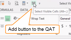
Please see the video for step-by-step instructions on how to add this button to the QAT. Pressing the button will select visible cells only. It also shows the keyboard shortcut when you hover your mouse over the button.

The Go To Special Menu

You can also find the Select Visible Cells Only option on the Go To Special menu.

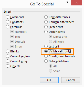
This can be a very useful menu for selecting other types of cells besides just visible cells. As you can see in the image above there are a lot of options for different types of cells you can select.

There are a few different ways to open the Go To Special menu.

1. On the Home Tab of the Ribbon, press the Find & Select button on the far right side. Then choose Go To Special…

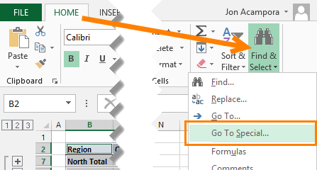
2. Press Ctrl+G or the F5 key on the keyboard from anywhere in a worksheet. Then press the Special button.

So Many Different Ways to Select Visible Cells

As you can see, there are a lot of different ways to select the visible cells in Excel. For me, the keyboard shortcut (Alt+;) is by far the fastest. If you don’t think you’ll remember it then put the button on the QAT. 🙂

Either way, this is one shortcut that should help save you a lot of time!

Paste to the Visible Cells Only

If you have ever received the following error message in Excel, “The command cannot be used on multiple selections”, then you know that you cannot paste to the visible cells in range that contains hidden rows or columns. This is a limitation of Excel, and it can be frustrating.

The video below explains two workarounds for this.

Click the following link to learn more about the Paste Visible feature and download a free trial of the Paste Buddy add-in.

Click here to get Paste Buddy

Copy Visible Cells to Outlook Email

Mandy asked a great question in the comments below about how to paste the visible cells to an email in Outlook. The following screencast animation shows how to do this.

Here are the steps to copy the visible cells to an email :

Select visible cells in Excel – Alt+;
Copy the range – Ctrl+C
Open an email in Outlook
Choose from the Paste Options on the Message tab

The Paste button on the Message tab of the Ribbon contains a small drop-down arrow underneath it. Click this arrow to see the Paste Options. You can hover over each of the options to get a preview of what the paste will look like in the email.

When copying and pasting from Excel to Outlook, I usually use either the “Picture” or “Keep Text Only” options. If I know the user will be copying the data out of Outlook, then it’s best to give them the text. If I know the user will only be looking at the data, then I will paste a picture because I know the formatting will remain in tact.

Please leave a comment below with any questions.

Источник

Speed Up Copying and Pasting Using These Great Tricks and Shortcuts in Microsoft Excel

by Avantix Learning Team | Updated April 10, 2021

Applies to: Microsoft^® Excel^® 2013, 2016, 2019 and 365 (Windows)

It’s surprising how much time you can save with a few tricks and shortcuts for copying and pasting in Microsoft Excel. Here are 10 useful copy and paste shortcuts for Excel users.

Recommended article: 10 Excel Data Entry Tricks and Shortcuts Every User Should Know

Do you want to learn more about Excel? Check out our virtual classroom or live classroom Excel courses >

For the following examples, if you are dragging, clicking or double-clicking, use the left mouse button.

1. Copying and pasting using Ctrl + C and Ctrl + V

The most popular shortcut for copying and pasting can be used in Excel and other programs as well. In Excel, select the cells you want to copy and press Ctrl + C. Click the top left cell where you wish to paste and press Ctrl + V. The copied selection is saved in the Clipboard so you can continue pressing Ctrl + V in different locations if you want to make multiple copies of the selection.

2. Copying and pasting using Paste Special

Paste Special is a very useful tool in Excel. Many options from Paste Special appear when you copy and then right-click a cell (such as values). However, you can also access Paste Special using your keyboard.

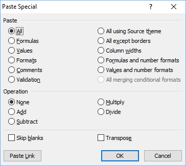
Select the cells you want to copy and press Ctrl + C. Click the top left cell where you wish to paste and press Ctrl + Alt + V. The Paste Special dialog box appears. Select an option (such as Values) and click OK.

3. Copying formulas down quickly

Instead of dragging the Fill handle on the bottom right corner of a cell to copy a formula down, select the cell with the formula you want to copy and double-click the handle on the bottom right corner. Excel will copy the formula down as long as there is data on the left.

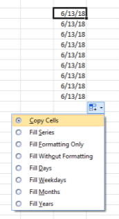
4. Copying a date

It’s common for Excel users to drag the Fill handle on the bottom right corner of a cell to copy a date. However, if you drag the Fill handle of a cell containing a date, Excel assumes you want to generate a date series. If this occurs and you want to copy the date, click the Smart Tag that appears after you drag the Fill handle and select Copy Cells from the menu.

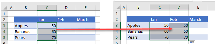
5. Copying using Drag and Drop

You can use Excel’s Drag and Drop pointer to copy a cell or range of cells. Simply select a cell or a range of cells and point to the border of the cell or range (not the corner). The pointer changes to the Drag and Drop pointer. Press Ctrl and drag the border of the cell or range to a new location. Release the mouse button and then release Ctrl. Excel will create a copy in the new location.

You can also use the Drag and Drop pointer to copy to another sheet. Select a cell or a range of cells and point to the border of the cell or range. The pointer changes to the Drag and Drop pointer. Press Ctrl + Alt and drag the border of the cell or range to a sheet tab to activate the sheet and then drag to a new location. Release the mouse button and then release Ctrl + Alt. Excel will create a copy in the new location on the other sheet.

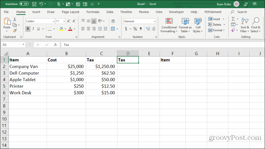
6. Copying from the cell above

To copy the data or formula from the cell above, click the cell below the cell you want to copy and press Ctrl + ‘ (apostrophe) or Ctrl + D.

7. Copying the value only from the cell above

To copy the value only (not the formula) from the cell above, click the cell below the cell you want to copy and press Ctrl + Shift + ‘ (apostrophe).

8. Copying from the cell to the left

To copy the data or formula from the cell to the left, click in the cell to the right of the cell and you want to copy and press Ctrl + R.

9. Copying formatting

To copy formatting from one cell to another:

Click the cell with the formatting you want to copy.
Click the Home tab in the Ribbon.
Click the Format Painter in the Clipboard group.
Click the cell to which you want to copy the formatting.

The Format Painter appears on the left in the Home tab in the Ribbon:

To copy formatting from one cell to many other cells:

Click the cell with the formatting you want to copy.
Click the Home tab in the Ribbon.
Double-click the Format Painter in the Clipboard group.
Click the cells to which you want to copy the formatting.
Press ESC or click the Format Painter to turn it off.

10. Copying a sheet

To quickly copy a sheet, point to the sheet tab you want to copy and then press Ctrl and drag the sheet to the right or left of the sheet tab. A sheet icon with a plus sign appears. Release the mouse button and then release Ctrl when the copy is in the desired location.

Subscribe to get more articles like this one

Did you find this article helpful? If you would like to receive new articles, join our email list.

More resources

How to Quickly Delete Blank Rows in Excel (5 Ways)

How to Fill or Replace Blank Cells in Excel with a Value from a Cell Above

How to Use Flash Fill in Excel to Clean or Extract Data (Beginner’s Guide)

How to Use Conditional Formatting in Excel to Highlight Dates Before Today (3 Ways)

Related courses

Microsoft Excel: Intermediate / Advanced

Microsoft Excel: Data Analysis with Functions, Dashboards and What-If Analysis Tools

Microsoft Excel: Introduction to Visual Basic for Applications (VBA)

VIEW MORE COURSES >

Our instructor-led courses are delivered in virtual classroom format or at our downtown Toronto location at 18 King Street East, Suite 1400, Toronto, Ontario, Canada (some in-person classroom courses may also be delivered at an alternate downtown Toronto location). Contact us at info@avantixlearning.ca if you’d like to arrange custom instructor-led virtual classroom or onsite training on a date that’s convenient for you.

Microsoft, the Microsoft logo, Microsoft Office and related Microsoft applications and logos are registered trademarks of Microsoft Corporation in Canada, US and other countries. All other trademarks are the property of the registered owners.

Avantix Learning |18 King Street East, Suite 1400, Toronto, Ontario, Canada M5C 1C4 | Contact us at info@avantixlearning.ca

Источник

Need more help?

See Also

Need more help?

Want more options?

Copy and Paste Multiple Adjacent Cells

Useful Keyboard Shortcuts for Copy Paste

Mouse Shortcut for Copy Paste

Copy and Paste Multiple Non-Adjacent Cells

Copy and Paste Multiple Non-Adjacent Cells (that are in the same row/column)

Copy and Paste Multiple Non-Adjacent Rows/Columns (but adjacent cells)

Copy Value From Above in Non-Adjacent Cells

Select All Blank Cells in the Dataset

Fill Blank Cells with Value Above

How to Copy and Paste in Excel – Step-By-Step (2023)

How to copy and paste into Excel

1. The clipboard group

2. The right-click menu

3. The CTRL button

How to copy formulas only in Excel

How to make a copy of an Excel sheet

The right-click context menu:

Using the CTRL key:

Copy values not formula

Shortcut to paste values

How to copy formatting

That’s it – Now what?

Copy Adjacent Cells

Fill Handle

Quick Menu

Copy Nonadjacent Cells

Copy Entire Columns and/or Rows

Copy Formulas

Copy Cell Data or Formula

Copy a Formula to Adjacent Cells

Notes

Copy-Paste Multiple Cells in Google Sheets

Adjacent Cells

Nonadjacent Cells

Copy Entire Columns and Rows

More Options

1. Copy Formula Results

2. Copy Formulas Without Changing References

3. Avoid Copying Hidden Cells

4. Fill to Bottom with Formula

5. Copy Using Drag and Drop

6. Copy from Cell Above

7. Copy from Left Cell

8. Copy Cell Formatting

9. Copy Entire Sheet

10. Repeat Fill

11. Paste Entire Blank Column or Row

12. Paste Multiples of a Single Cell

13. Copy Column Width

14. Paste with Calculation

15. Transpose Column to Row

Why does Copy and Paste include hidden data in Excel?

Copying data that has hidden rows

Copying and pasting visible cells only in Excel (excluding hidden cells)

Excel Shortcuts for Copying and Pasting visible cells only (excluding hidden cells)

To Sum up

Instructions

Copying and pasting visible cells only in Excel (excluding hidden cells)

Excel Shortcuts for Copying and Pasting visible cells only (excluding hidden cells)

Notes

Why does Copy and Paste include hidden data in Excel?

Copying and pasting visible cells only in Excel (excluding hidden cells)

Elevate your Excel game and become a pro with our exclusive Insider Group.

Example Data

Paste Special Keyboard Shortcut

Paste Special Legacy Keyboard Shortcut

Paste Special Values Keyboard Shortcut

Paste Special from the Home Tab

Paste Values with Hotkey Shortcuts

Paste Values from Right Click Menu

Paste Values with Quick Access Toolbar Command

Paste Values Mouse Trick

Paste Values with Paste Options

Paste Values and Formulas with Text to Columns

Paste Values with Advanced Filters

Conclusions