Copy all visible cells excel - Word и Excel - помощь в работе с программами

If some cells, rows, or columns on a worksheet do not appear, you have the option of copying all cells—or only the visible cells. By default, Excel copies hidden or filtered cells in addition to visible cells. If this is not what you want, follow the steps in this article to copy visible cells only. For example, you can choose to copy only the summary data from an outlined worksheet.

Follow these steps:

Select the cells that you want to copy For more information, see Select cells, ranges, rows, or columns on a worksheet.

Tip: To cancel a selection of cells, click any cell in the worksheet.
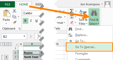
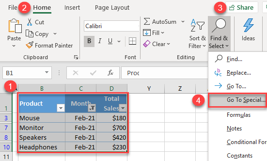
Click Home > Find & Select, and pick Go To Special.
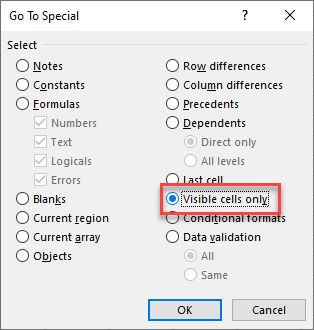
Click Visible cells only > OK.
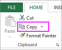
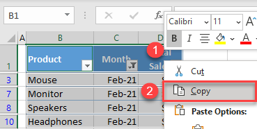
Click Copy (or press Ctrl+C).
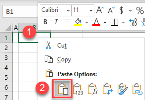
Select the upper-left cell of the paste area and click Paste (or press Ctrl+V).

Tip: To copy a selection to a different worksheet or workbook, click another worksheet tab or switch to another workbook, and then select the upper-left cell of the paste area.

Note: Excel pastes the copied data into consecutive rows or columns. If the paste area contains hidden rows or columns, you might have to unhide the paste area to see all of the copied cells.

When you copy and paste visible cells in a range of data that has hidden cells or filtering applied, you’ll notice that the hidden cells are pasted along with the visible ones. Unfortunately, you can’t change this when you copy and paste a range of cells in Excel for the web because the option to paste only visible cells isn’t available.

However, if the data is formatted as a table with filtering applied, you can copy and paste only the visible cells.

If you don’t want to format the data as a table and if you have the Excel desktop application, you can open your workbook to copy and paste the visible cells there. To do that, click Open in Excel and follow the steps in Copy and paste visible cells only.

Источник

Learn how to copy and paste excluding hidden columns or rows in Excel.

Ever tried to copy and paste data thinking you will be pasting, excluding the hidden columns or rows only to have the hidden data copied too?

Copying a data range that contains hidden data can be challenging when the hidden data travels with the copied range.

In this post I’ll explain how to copy and paste the visible cells only – hidden cells are excluded.

This blog includes step-by-step help on the following:

Why does Copy and Paste include hidden data in Excel?
Copying and pasting visible cells only in Excel (excluding hidden cells)
Excel Shortcuts for Copying and Pasting visible cells only (excluding hidden cells)

Why does Copy and Paste include hidden data in Excel?

Let’s look at what happens when we try to copy and paste a range with hidden data. In the example below we have an Excel spreadsheet with information on sales.

Excel Sales spreadsheet with information on sales made over the past year. Information includes Invoice # (Column A), Date (Column B), Customer Name (Column C), Product Name (Column D), Product Type (Column E), UOM (Column F), Cost Price (Column G), RRP (Column H), Sales Price (Column I), Quantity sold (Column J), Total Sales $ (Column K and Salesperson (Column L).

In this example, we are wanting to hide rows 6-9 and copy and paste the information in this data set without these rows included.

To follow along, rows 6-9 have been highlighted in yellow so that they are easily identified as we continue through the steps.

Excel Sales spreadsheet with columns 6-9 highlighted in yellow

To hide these rows, we will do the following.

Step 1: Select the rows we want hidden by clicking and dragging over the row numbers. In our example, this is rows 6-9.

Excel Sales spreadsheet with rows 6-9 highlighted and selected

Step 2: Right-click the selected rows and then select Hide from the menu.

List from right clicking with multiple options and mouse hovering over the Hide option

The rows we have selected will now be hidden.

You can see in our example, rows 6-9 are hidden. We can easily identify this as the highlighted rows are now hidden and the row numbers jump from 5 to 10.

Excel Sales spreadsheet with rows 6-9 hidden and a red box on the row tabs showing that they are hidden

Copying data that has hidden rows

Now let’s try copying the first 3 columns of data in this table to another worksheet. We are assuming that the hidden data will not copy because it is hidden.

Step 1: We will select the data range that we want to copy, including the hidden rows. In this example, we want to copy the Invoice number, Date and Customer Name columns.

Sales spreadsheet with columns Invoice # (Column A), Date (Column B) and Customer Name (Column C) are selected

Step 2: To copy the range we’ve selected, we will right-click the selected range and select Copy from the shortcut menu (or press Ctrl + C).

Shortcut menu with the mouse hovering over the Copy option

Step 3: We will now go to where we want to paste the data and select the cell that will be the top, left cell of the pasted range. In our example, we created a new sheet and are now wanting to paste the copied data into cell A3. The name of our new sheet is Sheet1 as this was the default name given to the sheet by Excel.

Sheet1 in the workbook with cell A3 selected

Step 4: We will now paste the copied data by doing a right-click and selecting Paste from the shortcut menu (or we can press Ctrl + V).

Shortcut menu with the mouse hovering over the paste option

Step 5: Unfortunately, we can see that the hidden data has been copied and included when we paste. This is easily identifiable as you can see the rows we highlighted in yellow, prior to doing the copy, have also copied over.

Sheet1 with pasted information and rows 6-9 are highlighted in yellow

This is because when we selected the data to be copied in Step 1, we are actually selecting both visible AND hidden data.

Therefore, when we copied we are copied ALL the data, not just the visible cells.

Most of the time this is not ideal, and you don’t want these hidden rows to travel over with the data you are copying and pasting.

The following steps will teach you how to paste visible cells only in Excel, excluding any hidden rows or columns.

Copying and pasting visible cells only in Excel (excluding hidden cells)

Step 1: Start by selecting the area you want to copy. In our example we will select the Invoice, Date and Customer Name columns. The highlighted rows 6 to 9 are hidden.

Sales spreadsheet with columns Invoice # (column A), Sale (Column B) and Customer Name (Column C) all highlighted

Step 2: From the Home tab, select Find & Select.

Home tab in Excel with a red box showing where Find & Select is

Step 3: Select Go To Special.

Find & Select is selected with the mouse hovering over the Go To Special option

The Go To Special dialogue box will appear.

Go To Special Dialogue box with Notes selected

Step 4: Select Visible cells only. This ensures only the visible cells are included in your selection. The hidden cells are excluded.

Go To Special dialogue box with Visible cells only selected

Step 5: Click OK.

Go To Special dialogue box with Visible cells only selected and the mouse over OK

You will now see that the visible cells have been selected and the hidden cells are excluded. A small line within the selected area shows this .

A red box showing where there is a small line indicating that there are rows hidden in this area. The line is between rows 5 and 10

Step 6: Now Copy the selected cells by right-clicking over the selected area and selecting Copy from the shortcut menu (or press Ctrl + C).

Columns A B and C are selected with shortcut menu and mouse over the option Copy

Step 7: Go to where you want to paste the data and select the cell that will be the top, left cell of the pasted range. In our example, we created a new sheet called Sheet 1 as this is the default name given by Excel and we selected cell A3.

Sheet1 with cell A3 selected

Step 8:
Paste by doing a right-click and selecting Paste from the shortcut menu (or press Ctrl + V).

Shortcut menu with the mouse over the Paste option

Super Tip: If you want to paste your cells with the exact same column widths as the sheet they were copied from, when you go to paste do a right-click and select Paste Special. From there, select Keep Source Column Widths (W).

Only the visible cells will be pasted.

In this example, we can easily tell that only the visible cells have been pasted as the hidden rows were highlighted in yellow and they have not appeared.

Sheet1 in the workbook with Invoice # information starting in cell A3, Date information starting in cell B3 and Customer Name information starting in tow C3

Excel Shortcuts for Copying and Pasting visible cells only (excluding hidden cells)

1. Select the range to be copied, including the hidden data.

2. Press ALT + ; (ALT + semicolon to select only visible data and exclude any hidden data)

3. Press Ctrl + C (to copy)

4. Go to where you want to paste the data and select the cell that will be the top, left cell of the pasted range.

5. Press Ctrl + V (to paste the data).

To Sum up

The trick is to ensure you are only selecting visible cells prior to doing your Copy.

Once you have this mastered you can easily control your data and copy visible cells only.

Was this blog helpful? We’d love to know. If you’re a beginner or if you use Excel every day please let us know if we helped in some way by leaving a Comment below.

Instructions

Copying and pasting visible cells only in Excel (excluding hidden cells)

Select the area you want to copy.
From the Home tab, select Find & Select.
Select Go To Special. The Go To Special dialogue box will appear.
Select Visible cells only. This ensures only the visible cells are included in your selection. The hidden cells are excluded.
Click OK. You will now see that the visible cells have been selected and the hidden cells are excluded. A small line within the selected area shows this.
Now Copy the selected cells by right-clicking over the selected area and selecting Copy from the shortcut menu (or press Ctrl + C).
Go to where you want to paste the data and select the cell that will be the top, left cell of the pasted range.
Paste by doing a right-click and selecting Paste from the shortcut menu (or press Ctrl + V).

Excel Shortcuts for Copying and Pasting visible cells only (excluding hidden cells)

Select the range to be copied, including the hidden data.
Press ALT + ; (ALT + semicolon to select only visible data and exclude any hidden data)
Press Ctrl + C (to copy)
Go to where you want to paste the data and select the cell that will be the top, left cell of the pasted range.
Press Ctrl + V (to paste the data).

Notes

Why does Copy and Paste include hidden data in Excel?

When you select a range that has hidden data, you are also selecting that hidden data. This means that when you copy and paste the data, the hidden data will be copied and pasted with it. If you want to copy and paste visible cells only, the trick is to ensure you are only selecting visible cells prior to doing your Copy.

Copying and pasting visible cells only in Excel (excluding hidden cells)

If you enjoyed this post check out the related posts below.

Elevate your Excel game and become a pro with our exclusive Insider Group.

Be the first to know about new tutorials, videos, and tips for Microsoft 365 products. Join us now and claim your exclusive bonus today!

Источник

Have you ever tried to copy and paste a range with hidden rows or columns and didn’t get the results you expected? This problem can be frustrating and time consuming! In this post and video I will explain how to solve this problem with a very simple shortcut to select the visible cells only.

Have you ever tried to copy and paste a range with hidden rows or columns and didn’t get the results you expected?

This problem can be frustrating and time consuming! In this post and video I will explain how to solve this problem with a very simple shortcut. The shortcut will select the visible cells only in a range, ignoring the hidden rows and columns.

Please leave a comment below with any questions.

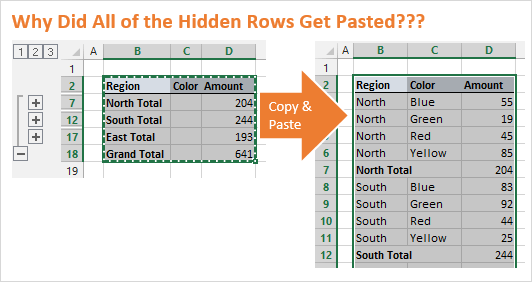
Why Are My Hidden Rows & Columns Being Pasted?

When you copy a range of cells that contains hidden rows or columns, Excel includes ALL of the selected rows. It does not matter if they are visible or hidden. When you go to paste the range, all the cells in the selection will be pasted.

This is actually a nice feature, but it’s not always what we are expecting to happen. Sometimes we only want to copy and paste the visible cells, and exclude the hidden rows & columns.

This commonly happens when you are working with a range that has filters applied to it. Or when you have hidden rows or columns from a collapsed group in an outline. The Subtotals feature automatically creates row groupings that can cause rows to be hidden, as shown in the example above.

Select the Visible Cells Only

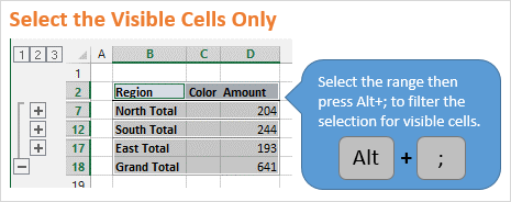
Excel gives us an option to select the visible cells only using the keyboard shortcut Alt+; (hold down the Alt key, then press the semi-colon key). The Mac shortcut is Cmd+Shift+Z.

This shortcut will exclude all the hidden rows and columns from the selection.

Copy & Paste Visible Cells

Here are instructions on how to copy and paste visible cells only (please see the video above for details):

Select the entire range you want to copy.
Press Alt+; to select the visible cells only. You will notice that the selection is cut up to skip the hidden rows and columns.
Copy the range – Press Ctrl+C or Right-click>Copy
Select the cell or range that you want to paste to
Paste the range – Press Ctrl+V or Right-click>Paste

Alternatives to Alt+;

If you don’t use this shortcut often then it might be hard to remember the keyboard shortcut. Here are a few alternatives for selecting visible cells.

Add a Button to the Quick Access Toolbar (QAT)

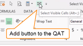
Please see the video for step-by-step instructions on how to add this button to the QAT. Pressing the button will select visible cells only. It also shows the keyboard shortcut when you hover your mouse over the button.

The Go To Special Menu

You can also find the Select Visible Cells Only option on the Go To Special menu.

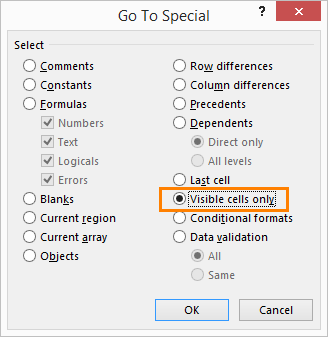
This can be a very useful menu for selecting other types of cells besides just visible cells. As you can see in the image above there are a lot of options for different types of cells you can select.

There are a few different ways to open the Go To Special menu.

1. On the Home Tab of the Ribbon, press the Find & Select button on the far right side. Then choose Go To Special…

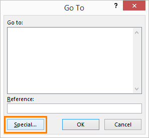
2. Press Ctrl+G or the F5 key on the keyboard from anywhere in a worksheet. Then press the Special button.

So Many Different Ways to Select Visible Cells

As you can see, there are a lot of different ways to select the visible cells in Excel. For me, the keyboard shortcut (Alt+;) is by far the fastest. If you don’t think you’ll remember it then put the button on the QAT. 🙂

Either way, this is one shortcut that should help save you a lot of time!

Paste to the Visible Cells Only

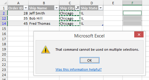
If you have ever received the following error message in Excel, “The command cannot be used on multiple selections”, then you know that you cannot paste to the visible cells in range that contains hidden rows or columns. This is a limitation of Excel, and it can be frustrating.

The video below explains two workarounds for this.

Click the following link to learn more about the Paste Visible feature and download a free trial of the Paste Buddy add-in.

Click here to get Paste Buddy

Copy Visible Cells to Outlook Email

Mandy asked a great question in the comments below about how to paste the visible cells to an email in Outlook. The following screencast animation shows how to do this.

Here are the steps to copy the visible cells to an email :

Select visible cells in Excel – Alt+;
Copy the range – Ctrl+C
Open an email in Outlook
Choose from the Paste Options on the Message tab

The Paste button on the Message tab of the Ribbon contains a small drop-down arrow underneath it. Click this arrow to see the Paste Options. You can hover over each of the options to get a preview of what the paste will look like in the email.

When copying and pasting from Excel to Outlook, I usually use either the “Picture” or “Keep Text Only” options. If I know the user will be copying the data out of Outlook, then it’s best to give them the text. If I know the user will only be looking at the data, then I will paste a picture because I know the formatting will remain in tact.

Please leave a comment below with any questions.

Источник

Содержание

Copy visible cells only
Need more help?
Move or copy cells, rows, and columns
Copy visible cells only
Need more help?
How to copy and paste visible cells in Excel – Excelchat
Steps to copy only visible cells
Instant Connection to an Expert through our Excelchat Service
How to Copy and Paste Only Visible Cells in Microsoft Excel
Default Copy and Paste With Hidden Cells in Excel
Copy Visible Cells Only in Excel

Copy visible cells only

Follow these steps:

Select the cells that you want to copy For more information, see Select cells, ranges, rows, or columns on a worksheet.

Tip: To cancel a selection of cells, click any cell in the worksheet.

Click Home > Find & Select, and pick Go To Special.

Click Visible cells only > OK.

Click Copy (or press Ctrl+C).

Select the upper-left cell of the paste area and click Paste (or press Ctrl+V).

Tip: To copy a selection to a different worksheet or workbook, click another worksheet tab or switch to another workbook, and then select the upper-left cell of the paste area.

Note: Excel pastes the copied data into consecutive rows or columns. If the paste area contains hidden rows or columns, you might have to unhide the paste area to see all of the copied cells.

However, if the data is formatted as a table with filtering applied, you can copy and paste only the visible cells.

If you don’t want to format the data as a table and if you have the Excel desktop application, you can open your workbook to copy and paste the visible cells there. To do that, click Open in Excel and follow the steps in Copy and paste visible cells only.

Need more help?

You can always ask an expert in the Excel Tech Community or get support in the Answers community.

Источник

Move or copy cells, rows, and columns

When you move or copy rows and columns, by default Excel moves or copies all data that they contain, including formulas and their resulting values, comments, cell formats, and hidden cells.

When you copy cells that contain a formula, the relative cell references are not adjusted. Therefore, the contents of cells and of any cells that point to them might display the #REF! error value. If that happens, you can adjust the references manually. For more information, see Detect errors in formulas.

You can use the Cut command or Copy command to move or copy selected cells, rows, and columns, but you can also move or copy them by using the mouse.

By default, Excel displays the Paste Options button. If you need to redisplay it, go to Advanced in Excel Options. For more information, see Advanced options.

Select the cell, row, or column that you want to move or copy.

Do one of the following:

To move rows or columns, on the Home tab, in the Clipboard group, click Cut or press CTRL+X.

To copy rows or columns, on the Home tab, in the Clipboard group, click Copy or press CTRL+C.

Right-click a row or column below or to the right of where you want to move or copy your selection, and then do one of the following:

When you are moving rows or columns, click Insert Cut Cells.

When you are copying rows or columns, click Insert Copied Cells.

Tip: To move or copy a selection to a different worksheet or workbook, click another worksheet tab or switch to another workbook, and then select the upper-left cell of the paste area.

Note: Excel displays an animated moving border around cells that were cut or copied. To cancel a moving border, press Esc.

By default, drag-and-drop editing is turned on so that you can use the mouse to move and copy cells.

Select the row or column that you want to move or copy.

Do one of the following:

Cut and replace Point to the border of the selection. When the pointer becomes a move pointer , drag the rows or columns to another location. Excel warns you if you are going to replace a column. Press Cancel to avoid replacing.

Copy and replace Hold down CTRL while you point to the border of the selection. When the pointer becomes a copy pointer , drag the rows or columns to another location. Excel doesn’t warn you if you are going to replace a column. Press CTRL+Z if you don’t want to replace a row or column.

Cut and insert Hold down SHIFT while you point to the border of the selection. When the pointer becomes a move pointer , drag the rows or columns to another location.

Copy and insert Hold down SHIFT and CTRL while you point to the border of the selection. When the pointer becomes a move pointer , drag the rows or columns to another location.

Note: Make sure that you hold down CTRL or SHIFT during the drag-and-drop operation. If you release CTRL or SHIFT before you release the mouse button, you will move the rows or columns instead of copying them.

Note: You cannot move or copy nonadjacent rows and columns by using the mouse.

Источник

Copy visible cells only

Follow these steps:

Select the cells that you want to copy For more information, see Select cells, ranges, rows, or columns on a worksheet.

Tip: To cancel a selection of cells, click any cell in the worksheet.

Click Home > Find & Select, and pick Go To Special.

Click Visible cells only > OK.

Click Copy (or press Ctrl+C).

Select the upper-left cell of the paste area and click Paste (or press Ctrl+V).

Tip: To copy a selection to a different worksheet or workbook, click another worksheet tab or switch to another workbook, and then select the upper-left cell of the paste area.

Note: Excel pastes the copied data into consecutive rows or columns. If the paste area contains hidden rows or columns, you might have to unhide the paste area to see all of the copied cells.

However, if the data is formatted as a table with filtering applied, you can copy and paste only the visible cells.

Need more help?

You can always ask an expert in the Excel Tech Community or get support in the Answers community.

Источник

How to copy and paste visible cells in Excel – Excelchat

When working on a worksheet, you might encounter a situation where some cells either do not appear or simply not visible. In such a situation, we have the option to select only visible cells . Note that by default, Excel will copy both visible and invisible cells .

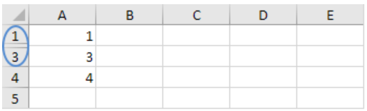Figure 1: Copy paste visible cells

In figure 1 above, we have row 2 invisible or hidden.

If we were to copy and paste the range in the above figure, we shall get result as shown in figure 2 below;

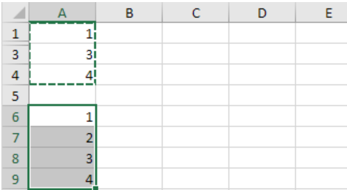Figure 2: Copy paste a range of cells

With this procedure, you might have noticed that we have copy/pasted both hidden as well as visible cells .

But what if we want to copy and paste only visible cells ? Well, we can select visible cells only in Excel 2010 and other versions by following a simple procedure as explained below;

Steps to copy only visible cells

In order to copy visible cells in Excel, follow the steps below;

Step 1: Select the range of visible cells you want to copy . In our example, the range is A1:A4

Step 2: Click Find & Select

To get the Find & Select tab, head to the Home tab, and under the Editing group , click on the Find & Select .

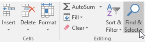Figure 3: Choose Find & Select

Step 3: Clock Go To Special

In the drop-down menu that appear, click “ Go To Special ”

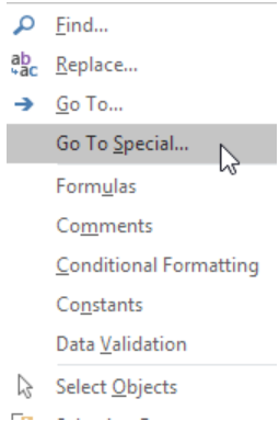Figure 4: Choose Go To Special

Step 4: Select Visible cells only

You will be presented with a window with various Go To Special options. Among the options is Visible cells only . Click on it and the click OK.

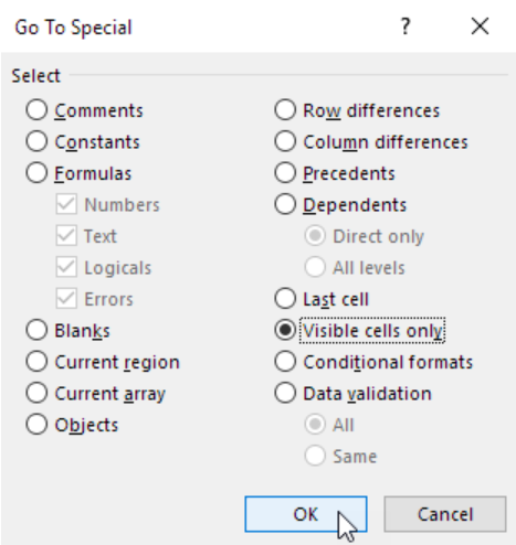Figure 5: Click ok

Step 5: Copy the range

The next thing you have to do is to copy the visible range . To do this, simply press Ctrl + C .

Step 6: Paste the range

Now that we have copied the visible cells , we now have to paste them. Pasting visible cells is actually easy, all we need to do is select where we want to paste them then press Ctrl + V .

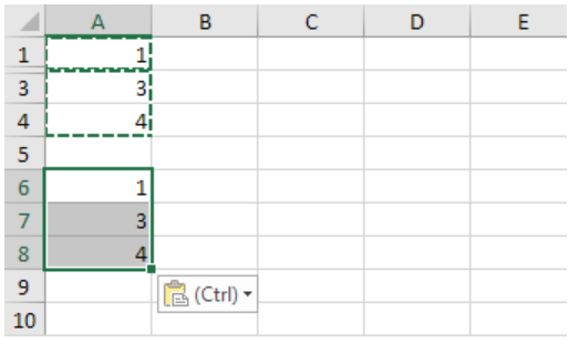Figure 6: Pasting the visible cells

Instant Connection to an Expert through our Excelchat Service

Most of the time, the problem you will need to solve will be more complex than a simple application of a formula or function. If you want to save hours of research and frustration, try our live Excelchat service! Our Excel Experts are available 24/7 to answer any Excel question you may have. We guarantee a connection within 30 seconds and a customized solution within 20 minutes.

Источник

How to Copy and Paste Only Visible Cells in Microsoft Excel

With her B.S. in Information Technology, Sandy worked for many years in the IT industry as a Project Manager, Department Manager, and PMO Lead. She learned how technology can enrich both professional and personal lives by using the right tools. And, she has shared those suggestions and how-tos on many websites over time. With thousands of articles under her belt, Sandy strives to help others use technology to their advantage. Read more.

You may hide columns, rows, or cells in Excel to make data entry or analysis easier. But when you copy and paste a cell range with hidden cells, they suddenly reappear, don’t they?

You might not realize it, but there is a way to copy and paste only the visible cells in Microsoft Excel. It takes nothing more than a few clicks.

By default, when you copy a cell range in Excel that contains hidden cells, those hidden cells display when you paste.

As an example, we’ve hidden rows 3 through 12 (February through November) in the following screenshot.

When we select the visible cell range, use the Copy action, and then Paste, those hidden cells appear.

If this isn’t what you want, read on for how to avoid it.

Copy Visible Cells Only in Excel

This nifty hidden feature is available in Microsoft Excel on both Windows and Mac. And luckily, it works exactly the same way.

Start by selecting the cells you want to copy and paste. Then, head to the Home tab and click the Find & Select (magnifying glass) drop-down arrow. Choose “Go To Special.”

In the window that appears, pick “Visible Cells Only” and click “OK.”

With the cells still selected, use the Copy action. You can press Ctrl+C on Windows, Command+C on Mac, right-click and pick “Copy,” or click “Copy” (two pages icon) in the ribbon on the Home tab.

Now move where you want to paste the cells and use the Paste action. You can press Ctrl+V on Windows, Command+V on Mac, right-click and pick “Paste,” or click “Paste” in the ribbon on the Home tab.

You should then see only the visible cells from your cell selection pasted.

If you perform actions like this in Word often, be sure to check out our how-to for cutting, copying, and pasting in Microsoft Word.

Источник

To dynamically copy visible cells only in Excel 365, we can use a FILTER formula. It has certain advantages compared to manual methods.

Before going to that, let’s go to some non-formula/manual methods which are so popular.

What happens when you usually copy a cell range in Excel 365? To answer that, one must know how you have made some rows hidden in Excel 365.

Filtered Data

If the rows are hidden due to filtering using Data -> Filter, then you can copy visible cells only without any issues. Here is how.

1. Select the cell range.

2. Right-click and copy (Ctrl+C).

3. Then right-click and paste (Ctrl+V) it in the destination cell.

It’s hassle-free. But I don’t advise it as you may make errors if there are manually hidden rows with filtered out data. So better to follow the below steps.

Manually Hidden Rows in Data

When you have manually hidden rows, then to copy visible cells only in Excel 365, you can follow either of the below two methods.

Method 1

1. Select the cell range to copy.

2. In the Home tab, within the Editing group, click Find & Select -> Go To Special (Ctrl+G, Alt+S).

3. Toggle “Visible cells only.”

4. Click “OK.”

5. Then copy and paste as earlier (Ctrl+C, Ctrl+V)

Method 2

Go to the first cell in the top left corner of your cell range to copy.

Press and hold the key Alt+;

Use your mouse to highlight the area to copy.

Then copy-paste (Ctrl+C, Ctrl+V) as earlier.

Pros and Cos of Manually Copying Visible Cells Only In Excel 365

Pros:

1. No formula or coding required. So even a novice Excel 365 user can follow these methods.

2. The copy-pasted values won’t update when you modify the source range.

Cons:

1. Point # 2 is the main drawback of the above method. The above is not a dynamic way.

When you modify the source, you may require to follow the above steps each time.

You can automate this process using a Filter formula. Below you can find the dynamic way to copy visible cells only in Excel 365.

Formula to Copy Visible Cells Only In Excel 365

I have data in A1:C11, and in that, I have hidden some of the rows.

Here visible cells can be the rows left after hiding manually or using the Data -> Filter.

We need to find a way to identify the rows that are hidden manually or using the Data -> Filter.

So that, we can use that as a condition in a FILTER formula.

Here is the syntax of the formula to dynamically copy visible cells only in Excel 365.

=FILTER(cell_range_to_copy,row_id=1)

In the above example, the range to copy is A2:C11. What about row_id?

It’s the below formula.

=SUBTOTAL(103,OFFSET(A2,ROW(A2:A11)-MIN(ROW(A2:A11)),0))

You can find this Excel 365 formula explanation here – How to Exclude Hidden Rows Conditionally in Formulas in Excel 365.

As per the above syntax, we can code the formula below to copy visible cells only in Excel 365.

=FILTER('VR'!A2:C11,SUBTOTAL(103,OFFSET('VR'!A2,ROW('VR'!A2:A11)-MIN(ROW('VR'!A2:A11)),0))=1)

Replace VR in the above Excel formula with the tab name in which your source data resides.

Here are the pros and cons of the above Excel formula approach.

Pros and Cons of Formula Approach

Pros:

1. You can see the changes in the source immediately in the copied range (formula result). It can be the changes in values, hiding more rows, etc.

2. You have the option to always manually copy the formula result to a new range to avoid changes.

3. Very easy to include several rows and columns in the range to copy, excluding hidden cells.

Cons:

1. The above first advantage can be a disadvantage for some users.

I have explained different options to copy visible cells only in Excel 365. Which one do you prefer – the dynamic one or the manual methods?

Excel 365 Filter Resources:

How to Use Wildcards in Filter Function in Excel (Alternatives).
How to Get Title Row with Filter Formula Result in Excel.
Not Equal to in Filter Function in Excel.
Filter Nth Occurrence in Excel 365 (Formula Approach).

Источник

Have you ever wanted to only copy or paste visible cells?

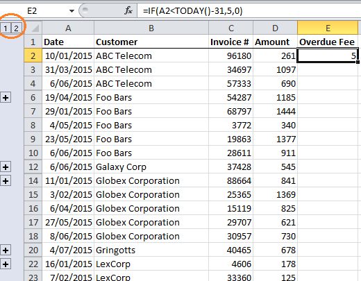
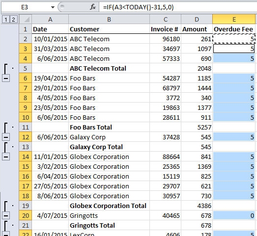
For example, below I have a table containing outstanding customer invoices. I want to insert a formula in column E to insert an overdue fee for invoices outstanding longer than 31 days:

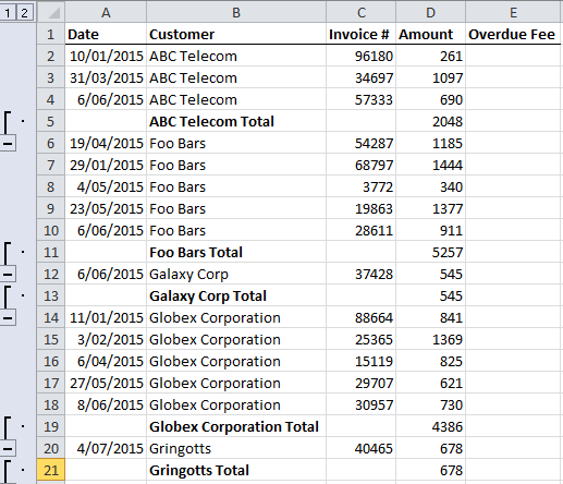
However, I don’t want the formula on the subtotal rows (row 5, 11, 13, 19, 21 etc.)

I can use the Group buttons to quickly hide the subtotal rows. I’ve entered my formula in cell E2 and I just need to copy it down:

Note: The method of hiding the rows doesn’t make any difference to how this technique works. You could use filters, or a regular right-click on the row label > Hide, to hide the Subtotal rows. I used the Group tool on the Data tab of the ribbon so I could easily hide/unhide the rows for the purpose of writing this tutorial quickly.

The problem with a regular copy and paste is Excel will also paste to the hidden cells, so I have to select the visible cells first. I can do this with Go To Special:

Copy cell E2 to the clipboard – just select it and press CTRL+C
Select the range you want to paste to. In my case E3:E51
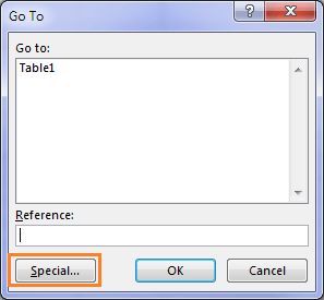
Press CTRL+G to open the Go To dialog box and then click ‘Special’ in the bottom left:
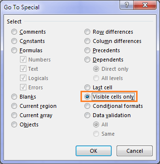
In the Go To Special dialog box select the ‘Visible cells only’ button and click OK.

Notice how each group of cells are individually selected:

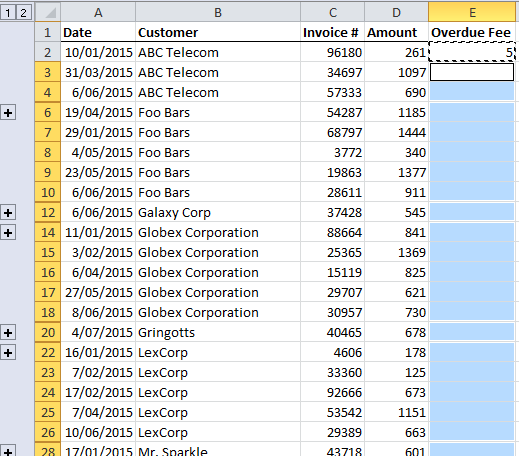
You can go ahead and press CTRL+V to paste the formula into the visible cells. I’ve unhidden the subtotal rows in the image below so you can see the magic:

Tip: Instead of copying and pasting, I could enter the same formula in all the selected visible cells using steps 2 to 4 above, then for step 5: type in the formula and press CTRL+ENTER to enter them all in one go.

Copy Visible Cells Only

Copying cells in a filtered table will only copy the visible cells by default, but if you have hidden rows or columns (as opposed to filtered), then Excel will copy the hidden ones too.

For example, you can see in the data below that row 3 is hidden:

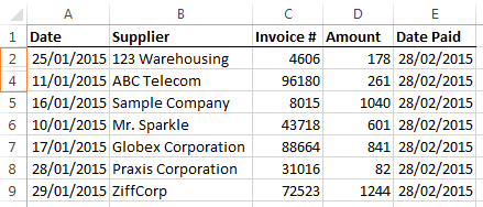
We can use the same technique to only copy visible cells:

Select the range A2:E9
CTRL+G to open the Go To dialog box
Click ‘Special’
Select ‘Visible cells only’

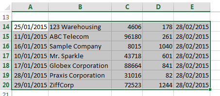
You can see there is a subtle line between rows 2 and 4 indicating row 3 is not selected:

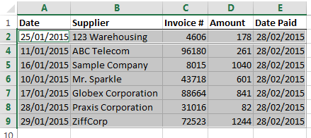
Press CTRL+C to copy and then go ahead and paste the cells where you want. You’ll notice they are pasted as a contiguous range of the 7 copied rows:

Filtered Tables

By default copying and pasting in filtered tables only does so for visible cells, although I have experienced occasions where this didn’t work as it should (but I couldn’t replicate it for this post 🙁 ), so I always use this technique, even in a filtered table.

Источник

See all How-To Articles

This tutorial demonstrates how to copy filtered (visible) data in Excel and Google Sheets.

Copy Filtered Data

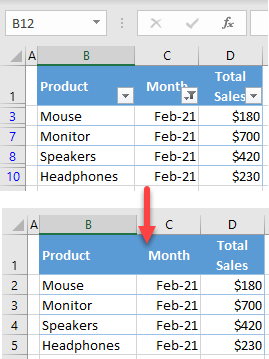
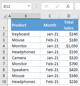
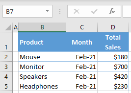
Say you have the following sales dataset and want to filter and copy only rows with Feb-21 in Column C (Month).

First, turn on AutoFilter arrows to be able to filter data.
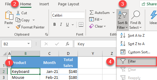
Click anywhere in the data range, and in the Ribbon, go to Home > Sort & Filter > Filter.

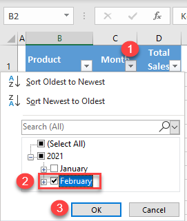
Now, click on the AutoFilter icon in Column C heading, tick February (under 2021), and click OK.

As a result of previous steps, only rows with the month Feb-2021 are filtered. To copy only visible cells, select the data range you want to copy (B1:D10), and in the Ribbon, go to Home > Find & Select > Go To Special…

In the Go To Special dialog box, check Visible cells only and click OK.

1. Now only visible cells (filtered data) are selected. Right-click anywhere in the selected area, and click Copy (or use the keyboard shortcut CTRL + C).

Right-click the cell where you want to paste the data, and choose Paste (or use the keyboard shortcut CTRL + V).

This copies only the filtered data (Feb-21).

Copy Filtered Data in Google Sheets

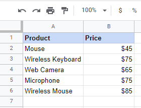
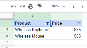
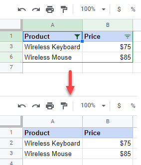
Say you have the following dataset and want to filter and copy only rows with the word Wireless in Column A (Product).

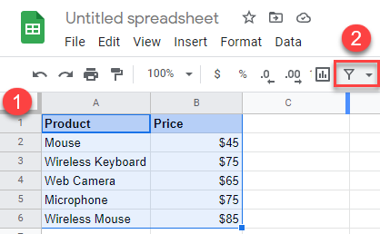
First, turn on filter arrows. Click anywhere in the data range, and in the Toolbar, click the Filter button.

Now, click on the Filter icon in the Column A heading, click on Filter by condition, and choose Text contains.

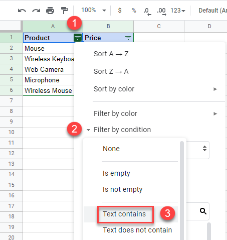
In the box enter the wanted text (in this example Wireless) and press OK.

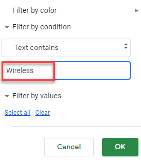
As a result, only rows with the word Wireless are visible.

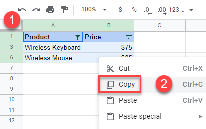
1. To copy only visible cells, select the data range you want to copy (A1:B6), right-click it, and choose Copy (or use the CTRL + C shortcut).

Select the cell where you want to paste the data, then right-click and click Paste.

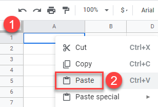
This copies over only filtered data.

Источник

In Microsoft Excel, we can easily copy the range of cells and paste it to some destination.

This can simply be done using the following steps.

Select the range of the cell
Copy the selected range using Ctrl + C command
Paste the copied cell to the destination using Ctrl + V command

But imagine a situation where we have some cells that are hidden in the range (like in the below example).

In the above data, rows 4 to 7 are hidden.

Now, if I copy this data that has hidden rows and paste it a few rows below it, something weird happens.

The hidden rows are also copied and pasted (as shown below)

By default, Excel copies the visible and hidden cells as shown in the above screenshot. So how to overcome this and only select the visible cell?

This tutorial will guide you through all the methods using which you can select the visible cell only in Excel.

Method 1: Keyboard Shortcut to Select Visible Cells Only

This is the easiest method to copy and paste the visible cell only in Excel.

Below is the keyboard shortcut to select the visible cells only:

ALT + ; (for windows)

Cmd + Shift + Z (for mac)

Let me explain it with the help of an example in which I am going to use the below dataset, where we have some Employee records with rows 4-7 hidden.

Let’s see how we can select the visible cell only. To achieve this, follow the below steps

Select the range of data that you want to copy.

Press the shortcut ALT + ; from the keyboard (hold the ALT key and then press the semicolon key). Remember the command for Mac users is Cmd + Shift + Z.

keyboard shortcut to only select visible sense

To copy the visible range, press Ctrl + C from the keyboard. Some dotted lines appear around the selection, as shown below.

Paste the cell to the destination using Ctrl + V command

copy and pasting when only visible cells are selected

This will paste only the visible cells and exclude the hidden cells, as you can see from the above screenshot.

There are other methods to perform this, which are discussed in the below sections.

Also read: How to Select Every Other Row (Alternate Row) in Excel?

Method 2: Select Visible Cells Only Using the Go to Special Dialog Box

Using the shortcut key (Alt + 😉 is a simple and easy way to copy only visible cells in Excel, but if you don’t want to remember the keyboard shortcut, you can do so by using the Go To Special option that is available in the Home tab of the ribbon.

Let me show you with the help of an example where I am going to use the same employee record data where rows 4-7 are hidden, as shown below.

Select the range of cells you want to copy.

Click on the Home tab in the ribbon

In the Home tab, click on the Find & Select option.

click the find and select option in the home tab

From the dropdown that gets open select the Go To Special option

This will open the Go To Special dialog box as shown below

Click on the option Visible cells only

select the visible cells only option in the go to special dialog box

Click on OK.

In this way, Excel will not follow the default copy-paste mechanism but only copy the visible cell.

To copy the selected range press Ctrl + C

Select the cell where you want to paste the range and press Ctrl + V

copy and pasting men only visible cells are selected

In this method, I showed you in great detail how you can use the Go To Special option to copy only visible cells.

There is another way you can do so, which is discussed in the below section.

Method 3: By Adding Select Visible Cells Option to Quick Access Toolbar

The above-discussed methods work perfectly for copying visible cells to the destination, but if you like to make it simpler, you can add the Select Visible Cells option to your Quick Access toolbar.

By doing so, you don’t have to remember the shortcut or the long process discussed in method 2.

In this method, first, I will explain how you can add a Select Visible Cells option to the toolbar, and then I will show you how you can quickly copy only visible cells using this option.

So follow all the steps to get a complete insight into the whole process.

a) Add the Select Visible Cells option to Quick Access Toolbar

Click on the Customizable Quick Access Toolbar option

click on the customizable quick access toolbar icon

From the dropdown that gets open, choose More Commands option

This will open Excel Options as shown below

Click on the ‘Choose commands from’ option

From the drop-down that gets opens, choose the “All Commands” option

select the all commands option from the drop down

This will show all the commands in Excel

Scroll down the command’s list and choose the Select Visible Cells option.

select the select visible cells only option

Click on Add

click on the add button to add the select visible sales icon to the quick access toolbar

Then click on OK

This will add the Select Visible Cells option to the toolbar as shown below

select visible sales icon is added to the quick access toolbar

b) Copy Visible Cell using the Select Visible Cells option

In the first part of this method, I showed you how you could add the Select Visible Cells option to your Quick Access Toolbar.

Now I will show you how you can employ this option to copy only visible cells just in a single click.

I am going to use the same dataset that is used in method 1 and method 2, where rows 4-7 are hidden.

Select the data that you want to copy.

Click on the Select Visible Cells icon in the Quick Access Toolbar (QAT)

click on the select visible sales icon in the quick access toolbar

Copy the data using Ctrl + C

Paste the data to the destination using Ctrl + V

copy and paste when visible cells are selected

This will only paste only the visible cell and exclude the hidden ones as shown in the above screenshot.

Tip: In the first part of this method, I also showed you how you could add the Select Visible Cells command to this Quick Access Toolbar. Similarly, you can also add any other command using the same process. Just look for the required command in the command’s list and add it using the procedure discussed in the above method.

If you’re a heavy Excel user, I am sure you will soon encounter this situation where you only need to select the visible cells (and not the hidden ones).

In this tutorial, I have discussed all the methods you can use to copy visible cells only.

I am personally a big fan of the keyboard shortcut, but in case you don’t want to burden yourself with yet another shortcut, you can add the select visible cells only icon in the Quick Access Toolbar and get this done with a single click.

Other Excel articles you may also like:

How to Select Non-adjacent Cells in Excel?
Select Row (or Rows) in Excel (Shortcut)
How to Select Rows with Specific Text in Excel
How to Select Multiple Items from a Drop Down in Excel?
How to Select Multiple Rows in Excel
How to Select Alternate Columns in Excel (or every Nth Column)
How to Select Every Other Cell in Excel (Or Every Nth Cell)
How to Paste in a Filtered Column Skipping the Hidden Cells

Источник

When working on a worksheet, you might encounter a situation where some cells either do not appear or simply not visible. In such a situation, we have the option to select only visible cells. Note that by default, Excel will copy both visible and invisible cells.

Figure 1: Copy paste visible cells

In figure 1 above, we have row 2 invisible or hidden.

If we were to copy and paste the range in the above figure, we shall get result as shown in figure 2 below;

Figure 2: Copy paste a range of cells

With this procedure, you might have noticed that we have copy/pasted both hidden as well as visible cells.

But what if we want to copy and paste only visible cells? Well, we can select visible cells only in Excel 2010 and other versions by following a simple procedure as explained below;

Steps to copy only visible cells

In order to copy visible cells in Excel, follow the steps below;

Step 1: Select the range of visible cells you want to copy. In our example, the range is A1:A4

Step 2: Click Find & Select

To get the Find & Select tab, head to the Home tab, and under the Editing group, click on the Find & Select.

Figure 3: Choose Find & Select

Step 3: Clock Go To Special

In the drop-down menu that appear, click “Go To Special”

Figure 4: Choose Go To Special

Step 4: Select Visible cells only

You will be presented with a window with various Go To Special options. Among the options is Visible cells only. Click on it and the click OK.

Figure 5: Click ok

Step 5: Copy the range

The next thing you have to do is to copy the visible range. To do this, simply press Ctrl + C.

Step 6: Paste the range

Now that we have copied the visible cells, we now have to paste them. Pasting visible cells is actually easy, all we need to do is select where we want to paste them then press Ctrl + V.

Figure 6: Pasting the visible cells

Instant Connection to an Expert through our Excelchat Service

Источник

After filtering, I want to copy all visible and non-empty cells (the cells which contain text). For some reason, my current code isn’t working. Any help would be greatly appreciated. Thanks!

  Sheets("Sheet1").Range("S2:S5000").SpecialCells(xlCellTypeVisible).SpecialCells(xlCellTypeConstants).Copy

asked Sep 4, 2013 at 23:33

Full admission that I did not try your code, but you can also try the following

With Sheets("Sheet1").Range("S2:S5000")
    Application.Intersect(.SpecialCells(xlCellTypeVisible), _
                       .SpecialCells(xlCellTypeConstants)).Copy
End With

Making the open ended assumption that the reason for copying is to paste somewhere else, you can update the above code by using

With Sheets("Sheet1").Range("S2:S5000")
    Application.Intersect(.SpecialCells(xlCellTypeVisible), _
          .SpecialCells(xlCellTypeConstants)).Copy _
               Destination:= Sheets("destSheet").Range("destRange")
End With

answered Sep 5, 2013 at 2:25

JaycalJaycal

2,0771 gold badge13 silver badges21 bronze badges

i need to copy all not empty, also one if there are not visible, but i find only this tread for. Eventualy is it usefull for someone…

Sub button_Klick()
On Error GoTo wrong
Dim r As Range
Dim sel As Range
'Dim f As Range
Dim text
Set r = Range("e4") 'd9:d1954

Set sel = Range(r)

'sel.SpecialCells(xlCellTypeConstants).Copy 'this will copy all, allso with formula =""

'Set f = Range("d9")'define first for union

For Each cell In sel.Cells
    If cell.Value <> "" Then
       'Set f = Union(f, cell)
       text = text & vbCrLf & cell.Value
    End If
Next cell
'f.Select
'f.Copy 'will copy allso all empty
Clipboard (text)
MsgBox "Ready!" & vbCrLf & "Text is in the clipboard...", vbInformation, "Ready! Text is in the clipboard..."
Exit Sub

wrong:
  
  MsgBox "Error " & vbCrLf & "Number: " & Err.Number & _
  vbCrLf & "Description: " & Err.Description
  'Application.Calculation = xlCalculationAutomatic
        
End Sub

'https://stackoverflow.com/questions/14219455/excel-vba-code-to-copy-a-specific-string-to-clipboard/60896244#60896244
Function Clipboard$(Optional s$)
    Dim v: v = s  'Cast to variant for 64-bit VBA support
    With CreateObject("htmlfile")
    With .parentWindow.clipboardData
        Select Case True
            Case Len(s): .setData "text", v
            Case Else:   Clipboard = .GetData("text")
        End Select
    End With
    End With
End Function

answered Apr 7, 2022 at 9:29

VivilVivil

395 bronze badges

Источник