The TEXT function lets you change the way a number appears by applying formatting to it with format codes. It’s useful in situations where you want to display numbers in a more readable format, or you want to combine numbers with text or symbols.
Note: The TEXT function will convert numbers to text, which may make it difficult to reference in later calculations. It’s best to keep your original value in one cell, then use the TEXT function in another cell. Then, if you need to build other formulas, always reference the original value and not the TEXT function result.
Syntax
TEXT(value, format_text)
The TEXT function syntax has the following arguments:
|
Argument Name |
Description |
|
value |
A numeric value that you want to be converted into text. |
|
format_text |
A text string that defines the formatting that you want to be applied to the supplied value. |
Overview
In its simplest form, the TEXT function says:
-
=TEXT(Value you want to format, «Format code you want to apply»)
Here are some popular examples, which you can copy directly into Excel to experiment with on your own. Notice the format codes within quotation marks.
|
Formula |
Description |
|
=TEXT(1234.567,«$#,##0.00») |
Currency with a thousands separator and 2 decimals, like $1,234.57. Note that Excel rounds the value to 2 decimal places. |
|
=TEXT(TODAY(),«MM/DD/YY») |
Today’s date in MM/DD/YY format, like 03/14/12 |
|
=TEXT(TODAY(),«DDDD») |
Today’s day of the week, like Monday |
|
=TEXT(NOW(),«H:MM AM/PM») |
Current time, like 1:29 PM |
|
=TEXT(0.285,«0.0%») |
Percentage, like 28.5% |
|
=TEXT(4.34 ,«# ?/?») |
Fraction, like 4 1/3 |
|
=TRIM(TEXT(0.34,«# ?/?»)) |
Fraction, like 1/3. Note this uses the TRIM function to remove the leading space with a decimal value. |
|
=TEXT(12200000,«0.00E+00») |
Scientific notation, like 1.22E+07 |
|
=TEXT(1234567898,«[<=9999999]###-####;(###) ###-####») |
Special (Phone number), like (123) 456-7898 |
|
=TEXT(1234,«0000000») |
Add leading zeros (0), like 0001234 |
|
=TEXT(123456,«##0° 00′ 00»») |
Custom — Latitude/Longitude |
Note: Although you can use the TEXT function to change formatting, it’s not the only way. You can change the format without a formula by pressing CTRL+1 (or 
Download our examples
You can download an example workbook with all of the TEXT function examples you’ll find in this article, plus some extras. You can follow along, or create your own TEXT function format codes.
Download Excel TEXT function examples
Other format codes that are available
You can use the Format Cells dialog to find the other available format codes:
-
Press Ctrl+1 (
+1 on the Mac) to bring up the Format Cells dialog.
-
Select the format you want from the Number tab.
-
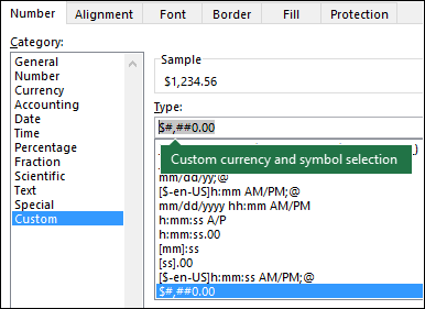
Select the Custom option,
-
The format code you want is now shown in the Type box. In this case, select everything from the Type box except the semicolon (;) and @ symbol. In the example below, we selected and copied just mm/dd/yy.
-
Press Ctrl+C to copy the format code, then press Cancel to dismiss the Format Cells dialog.
-
Now, all you need to do is press Ctrl+V to paste the format code into your TEXT formula, like: =TEXT(B2,»mm/dd/yy«). Make sure that you paste the format code within quotes («format code»), otherwise Excel will throw an error message.
Format codes by category
Following are some examples of how you can apply different number formats to your values by using the Format Cells dialog, then use the Custom option to copy those format codes to your TEXT function.
Why does Excel delete my leading 0’s?
Excel is trained to look for numbers being entered in cells, not numbers that look like text, like part numbers or SKU’s. To retain leading zeros, format the input range as Text before you paste or enter values. Select the column, or range where you’ll be putting the values, then use CTRL+1 to bring up the Format > Cells dialog and on the Number tab select Text. Now Excel will keep your leading 0’s.
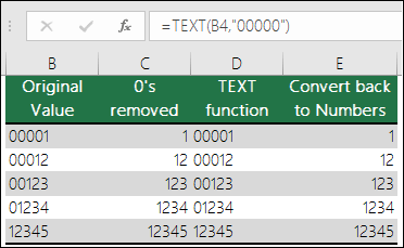
If you’ve already entered data and Excel has removed your leading 0’s, you can use the TEXT function to add them back. You can reference the top cell with the values and use =TEXT(value,»00000″), where the number of 0’s in the formula represents the total number of characters you want, then copy and paste to the rest of your range.
If for some reason you need to convert text values back to numbers you can multiply by 1, like =D4*1, or use the double-unary operator (—), like =—D4.
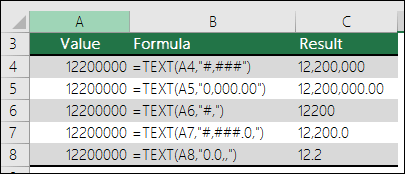
Excel separates thousands by commas if the format contains a comma (,) that is enclosed by number signs (#) or by zeros. For example, if the format string is «#,###», Excel displays the number 12200000 as 12,200,000.
A comma that follows a digit placeholder scales the number by 1,000. For example, if the format string is «#,###.0,», Excel displays the number 12200000 as 12,200.0.
Notes:
-
The thousands separator is dependent on your regional settings. In the US it’s a comma, but in other locales it might be a period (.).
-
The thousands separator is available for the number, currency and accounting formats.
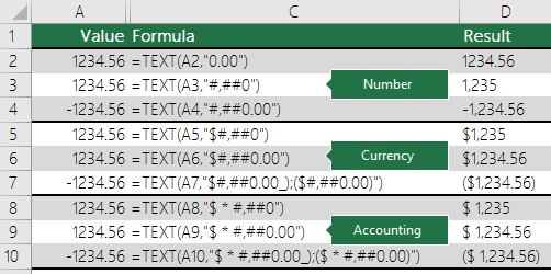
Following are examples of standard number (thousands separator and decimals only), currency and accounting formats. Currency format allows you to insert the currency symbol of your choice and aligns it next to your value, while accounting format will align the currency symbol to the left of the cell and the value to the right. Note the difference between the currency and accounting format codes below, where accounting uses an asterisk (*) to create separation between the symbol and the value.
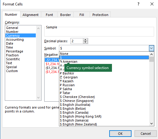
To find the format code for a currency symbol, first press Ctrl+1 (or 
Then click Custom on the left from the Category section, and copy the format code, including the currency symbol.
Note: The TEXT function does not support color formatting, so if you copy a number format code from the Format Cells dialog that includes a color, like this: $#,##0.00_);[Red]($#,##0.00), the TEXT function will accept the format code, but it won’t display the color.
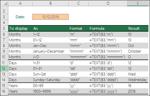
You can alter the way a date displays by using a mix of «M» for month, «D» for days, and «Y» for years.
Format codes in the TEXT function aren’t case sensitive, so you can use either «M» or «m», «D» or «d», «Y» or «y».
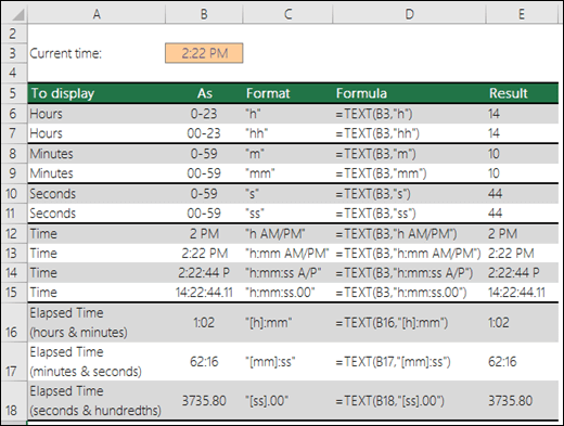
You can alter the way time displays by using a mix of «H» for hours, «M» for minutes, or «S» for seconds, and «AM/PM» for a 12-hour clock.
If you leave out the «AM/PM» or «A/P», then time will display based on a 24-hour clock.
Format codes in the TEXT function aren’t case sensitive, so you can use either «H» or «h», «M» or «m», «S» or «s», «AM/PM» or «am/pm».
You can alter the way decimal values display with percentage (%) formats.
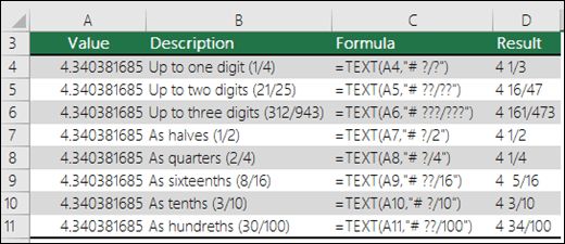
You can alter the way decimal values display with fraction (?/?) formats.
Scientific notation is a way of displaying numbers in terms of a decimal between 1 and 10, multiplied by a power of 10. It is often used to shorten the way that large numbers display.
Excel provides 4 special formats:
-
Zip Code — «00000»
-
Zip Code + 4 — «00000-0000»
-
Phone Number — «[<=9999999]###-####;(###) ###-####»
-
Social Security Number — «000-00-0000»
Special formats will be different depending on locale, but if there aren’t any special formats for your locale, or if these don’t meet your needs then you can create your own through the Format Cells > Custom dialog.
Common scenario
The TEXT function is rarely used by itself, and is most often used in conjunction with something else. Let’s say you want to combine text and a number value, like “Report Printed on: 03/14/12”, or “Weekly Revenue: $66,348.72”. You could type that into Excel manually, but that defeats the purpose of having Excel do it for you. Unfortunately, when you combine text and formatted numbers, like dates, times, currency, etc., Excel doesn’t know how you want to display them, so it drops the number formatting. This is where the TEXT function is invaluable, because it allows you to force Excel to format the values the way you want by using a format code, like «MM/DD/YY» for date format.
In the following example, you’ll see what happens if you try to join text and a number without using the TEXT function. In this case, we’re using the ampersand (&) to concatenate a text string, a space (» «), and a value with =A2&» «&B2.
As you can see, Excel removed the formatting from the date in cell B2. In the next example, you’ll see how the TEXT function lets you apply the format you want.
Our updated formula is:
-
Cell C2:=A2&» «&TEXT(B2,»mm/dd/yy») — Date format
Frequently Asked Questions
Yes, you can use the UPPER, LOWER and PROPER functions. For example, =UPPER(«hello») would return «HELLO».
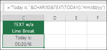
Yes, but it takes a few steps. First, select the cell or cells where you want this to happen and use Ctrl+1 to bring up the Format > Cells dialog, then Alignment > Text control > check the Wrap Text option. Next, adjust your completed TEXT function to include the ASCII function CHAR(10) where you want the line break. You might need to adjust your column width depending on how the final result aligns.
In this case, we used: =»Today is: «&CHAR(10)&TEXT(TODAY(),»mm/dd/yy»)
This is called Scientific Notation, and Excel will automatically convert numbers longer than 12 digits if a cell(s) is formatted as General, and 15 digits if a cell(s) is formatted as a Number. If you need to enter long numeric strings, but don’t want them converted, then format the cells in question as Text before you input or paste your values into Excel.
See Also
Create or delete a custom number format
Convert numbers stored as text to numbers
All Excel functions (by category)
Given an existing Excel 2003 document with cells of any type (integers, text, decimal, etc), how do I convert the contents of every cell to text?
And save all these changes in the same excel document?
asked Apr 13, 2010 at 18:29
Justin TannerJustin Tanner
6353 gold badges11 silver badges18 bronze badges
2
On a different sheet you can enter in cell A1:
="" & OriginalSheet!A1
Copy/Paste that for the full width and length of your original sheet. Then you can Paste Special>Values bock over the originals. That should make everything have your little green patch.
The only caveat is dates. When you apply this formula to a date field it will show the serial number of the date as text. Not the normal formatting you would have applied. To get around this, use this formula instead of the one above for date fields:
=TEXT(A1,"mm/dd/yyyy")
answered Apr 14, 2010 at 13:42
1
Here is the definitive answer:
highlight the numbers and use the Data > Text to Columns command. In Page 1 of the wizard, choose the appropriate type (this will probably be Delimited). In Page 2, remove any column dividers that may have shown up to keep the data in one column. In Page 3, click Text under Column data format to indicate that this column is text.
answered Apr 4, 2012 at 18:39
1
You can select all the fields, right click and copy, then right click and paste special/values. You probably want to copy into a new spreadsheet so you don’t lose your formulas.
Then select all the fields and do as Mark Robinson suggested: click Format Cells and chose text.
This will covert all formulas into the value they represent instead of a formula and then covert the values that are number into text.
answered Apr 13, 2010 at 20:40
Zooks64Zooks64
2,00214 silver badges14 bronze badges
4
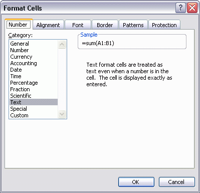
Select all your cells Ctrl+a
Right click on the selected cells and click Format Cells
Under the Number tab select Text as the Category
Text format cells are treated as text
even when a number is in the cell.
The cell is displayed exactly as
entered.
Then save your excel document
answered Apr 13, 2010 at 18:57
MarkMark
4783 silver badges12 bronze badges
1
The only way that I was able to overcome the problem of retaining only text from numbers and texts was to save my file as a .csv then close it and reopen it .. all data is then text and the file can then be saved as a .xlsx or whatever and formulae added. This enabled me to compare data from different sources and return values correctly.
answered Mar 6, 2021 at 18:51
Excel is a great tool which can be used for data entry, as a database, and to analyze data and create dashboards and reports.
While most of the in-built features and default settings are meant to be useful and save time for the users, sometimes, you may want to change things a little.
Converting your numbers into text is one such scenario.
In this tutorial, I will show you some easy ways to quickly convert numbers to text in Excel.
Why Convert Numbers to Text in Excel?
When working with numbers in Excel, it’s best to keep these as numbers only. But in some cases, having a number could actually be a problem.
Lets look at a couple of scenarios where having numbers creates issues for the users.
Keeping Leading Zeros
For example, if you enter 001 in a cell in Excel, you will notice that Excel automatically removes the leading zeros (as it thinks these are unnecessary).
While this is not an issue in most cases (as you wouldn’t leading zeros), in case you do need these then one of the solutions is to convert these numbers to text.
This way, you get exactly what you enter.
One common scenario where you might need this is when you’re working with large numbers – such as SSN or employee ids that have leading zeros.
Entering Large Numeric Values
Do you know that you can only enter a numeric value that is 15 digits long in Excel? If you enter a 16 digit long number, it will change the 16th digit to 0.
So if you are working with SSN, account numbers, or any other type of large numbers, there is a possibility that your input data is automatically being changed by Excel.
And what’s even worse is that you don’t get any prompt or error. It just changes the digits to 0 after the 15th digit.
Again, this is something that is taken care of if you convert the number to text.
Changing Numbers to Dates
This one erk a lot of people (including myself).
Try entering 01-01 in Excel and it will automatically change it to date (01 January of the current year).
So if you enter anything that is a valid date format in Excel, it would be converted to a date.
A lot of people reach out to me for this as they want to enter scores in Excel in this format, but end up getting frustrated when they see dates instead.
Again, changing the format of the cell from number to text will help keep the scores as is.
Now, let’s go ahead and have a look at some of the methods you can use to convert numbers to text in Excel.
Convert Numbers to Text in Excel
In this section, I will cover four different ways you can use to convert numbers to text in Excel.
Not all these methods are the same and some would be more suitable than others depending on your situation.
So let’s dive in!
Adding an Apostrophe
If you manually entering data in Excel and you don’t want your numbers to change the format automatically, here is a simple trick:
Add an apostrophe (‘) before the number
So if you want to enter 001, enter ‘001 (where there is an apostrophe before the number).
And don’t worry, the apostrophe is not visible in the cell. You will only see the number.

When you add an apostrophe before a number, it will change it to text and also add a small green triangle at the top left part of the cell (as shown in th image). It’s Exel way to letting you know that the cell has a number that has been converted to text.
When you add an apostrophe before a number, it tells Excel to consider whatever follows as text.
A quick way to visually confirm whether the cells are formatted as text or not is to see whether the numbers align to the left out to the right. When numbers are formatted as text, they align to the right by default (as they alight to the left)

Even if you add an apostrophe before a number in a cell in Excel, you can still use these as numbers in calculations
Similarly, if you want to enter 01-01, adding an apostrophe would make sure that it doesn’t get changed into a date.
Although this technique works in all cases, it is only useful if you’re manually entering a few numbers in Excel. If you enter a lot of data in a specific range of rows/columns, use the next method.
Converting Cell Format to Text
Another way to make sure that any numeric entry in Excel is considered a text value is by changing the format of the cell.
This way, you don’t have to worry about entering an apostrophe every time you manually enter the data.
You can go ahead entering the data just like you usually do, and Excel would make sure that your numbers are not changed.
Here is how to do this:
- Select the range or rows/column where you would be entering the data
- Click the Home tab

- In the Number group, click on the format drop down

- Select Text from the options that show up

The above steps would change the default formatting of the cells from General to Text.
Now, if you enter any number or any text string in these cells, it would automatically be considered as a text string.
This means that Excel would not automatically change the text you enter (such as truncating the leading zeros or converting entered numbers into dates)
In this example, while I changed the cell formatting first before entering the data, you can also do this with cells that already have data in them.
But remember that if you already had entered numbers that were changed by Excel (such as removing leading zeros or changing text to dates), that won’t come back. You will have to make that data entry again.
Also, keep in mind that cell formatting can change in case you copy and paste some data to these cells. With regular copy-paste, it also copied the formatting from the copied cells. So it’s best to copy and paste values only.
Using the TEXT Function
Excel has an in-built TEXT function that is meant to convert a numeric value to a text value (where you have to specify the format of the text in which you want to get the final result).
This method is useful when you already have a set of numbers and you want to show them in a more readable format or if you want to add some text as suffix or prefix to these numbers.
Suppose you have a set of numbers as shown below, and you want to show all these numbers as five-digit values (which means to add leading zeros to numbers that are less than 5 digits).

While Excel removes any leading zeros in numbers, you can use the below formula to get this:
=TEXT(A2,"00000")

In the above formula, I have used “00000” as the second argument, which tells the formula the format of the output I desire. In this example, 00000 would mean that I need all the numbers to be at least five-digit long.
You can do a lot more with the TEXT function – such as add currency symbol, add prefix or suffix to the numbers, or change the format to have comma or decimals.
Using this method can be useful when you already have the data in Excel and you want to format it in a specific way.
This can also be helpful in saving time when doing manual data entry, where you can quickly enter the data and then use the TEXT function to get it in the desired format.
Using Text to Columns
Another quick way to convert numbers to text in Excel is by using the Text to Columns wizard.
While the purpose of Text to Columns is to split the data into multiple columns, it has a setting that also allows us to quickly select a range of cells and convert all the numbers into text with a few clicks.
Suppose you have a data set is shown below, and you want to convert all the numbers in columns A into text.

Below are the steps to do this:
- Select the numbers in Column A
- Click the Data tab

- Click on the Text to Columns icon in the ribbon. This will open the text to columns wizard this will open the text to column wizard
- In Step 1 of 3, click the Next button
- In Step 2 of 3, click the Next button
- In Step 3 of 3, under the ‘Column data format’ options, select Text

- Click on Finish
The above steps would instantly convert all these numbers in Column A into text. You notice that the numbers would now be aligned to the right (indicating that the cell content is text).

There would also be a small green triangle at the top left part of the cell, which is a way Excel informs you that there are numbers that are stored as text.
So these are four easy ways that you can use to quickly convert numbers to text in Excel.
In case you only want this for a few cells where you would be manually entering the data, I suggest you use the apostrophe method. If you need to do data entry for more than a few cells, you can try changing the format of the cells from General to Text.
And in case you already have the numbers in Excel and you want to convert them to text, you can use the TEXT formula method or the Text to Columns method I covered in this tutorial.
I hope you found this tutorial useful.
Other Excel tutorials you may also like:
- Convert Text to Numbers in Excel
- How to Convert Serial Numbers to Dates in Excel
- Convert Date to Text in Excel – Explained with Examples
- How to Convert Formulas to Values in Excel
- Convert Time to Decimal Number in Excel
- How to Convert Inches to MM, CM, or Feet in Excel?
- Convert Scientific Notation to Number or Text in Excel
- Separate Text and Numbers in Excel
Skip to content
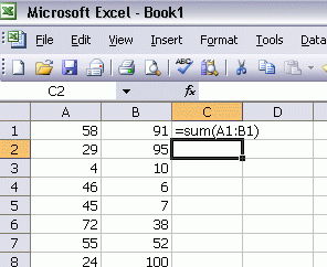
Excel has a Text format that can be applied to cells. When a cell is formatted as Text, anything you type in the cell will appears in the cell. That may seem obvious, but it applies to numbers and formulas too. For instance, if you type a formula in a cell formatted as Text, you see the formula rather than the result.
To remedy this, change the format to General (or something else), go into Edit mode in that cell, then exit the cell. Changing the format alone won’t fix the problem, you have to re-enter the cell. The easiest way to do this is to press F2 then Enter. F2 to edit the cell and Enter to commit the changes, even though you didn’t make any changes. This causes Excel to reevaluate the cell and show the proper result.
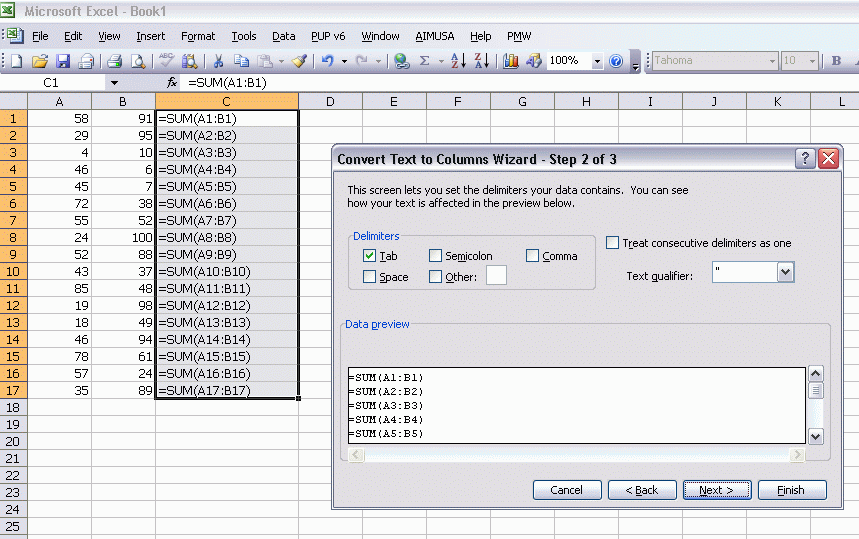
Kathy, however, does it differently. Instead of F2/Enter, she uses Data – Text to Columns, which also causes Excel to reevaluate the cell contents and formatting. When I asked her why, she said that while F2/Enter may be faster for one or two cells, TTC is better for a larger range.
By using Data – Text to Columns and specifying a delimiter that doesn’t exist (in this case, Tab is the delimiter and there are no tabs in the cells), each cell is written back to itself.
If you have a large range of formulas in Text formatted cells, remember the Text to Columns trick.
For converting numbers to text in Excel, there are two different methods:
- Method #1 – Use the “TEXT” function in Excel
- Method #2 – Use the “Format Cells” option
Now, let us discuss each of the methods with an example.
Table of contents
- How to Convert Numbers to Text in Excel?
- #1 Convert Numbers to Text using Excel TEXT Function
- #2 Convert Numbers to Text using Excel Format Cell Option
- Where can you Convert Numbers to Text in Excel?
- Example #1
- Example #2
- Recommended Articles
You can download this Convert Numbers to Text in Excel Template here – Convert Numbers to Text in Excel Template
#1 Convert Numbers to Text using Excel TEXT Function
The TEXT functionTEXT function in excel is a string function used to change a given input to the text provided in a specified number format. It is used when we large data sets from multiple users and the formats are different.read more converts numbers formatted as numbers to text in the specified format in Excel.
TEXT Formula in Excel
Arguments
value: The value for which text formatting is required
format_code: The formatting code is necessary for a number
The value can be any number. It can be entered directly or as a cell reference. It can also be a mathematical operation or a date. You could also specify TODAY() or MONTH() etc. in the value.
There are various format_code available in Excel. The format_code is always given in a double quotation mark. For example, you can use “0” to specify an integer with zero decimal place, “0.000” to specify three decimal places, “0000” to add leading zerosLeading zeros are zeros that are added to figures without altering their mathematical values. This is done to keep a specific format in a sheet or to prevent errors. We may add Leading Zeros in Excel by utilizing the Right, TEXT, and Concatenate Functions.read more, etc. We can also select percentages, scientific notations, currency, degrees, date formats in the TEXT function, such as “0.00%”, “$0”, “##0° 00′ 00″”, “DD/MM/YYYY.”
Returns
The function returns a number as text in the specified format.
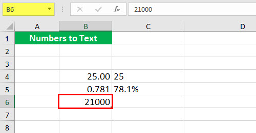
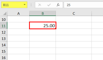
Suppose you have cell B4 containing the number 25.00 and formatted as a number. You want to convert numbers to text format.
You may give the TEXT formula as:
= TEXT (B4, “0”)
It will return the number in text format.
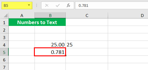
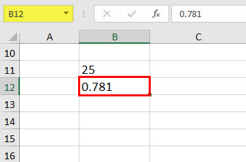
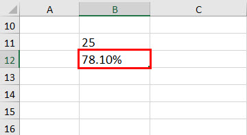
Suppose we have a number as 0.781 in cell B5. We want to convert this number to a percentage.
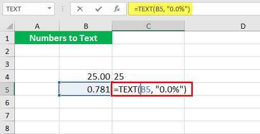
We can use the following TEXT formula:
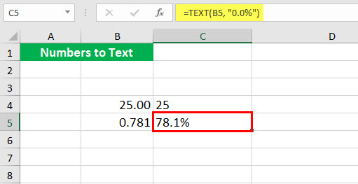
= TEXT (B5, “0.0%”)
As a result, it will return 78.1% as a TEXT format.
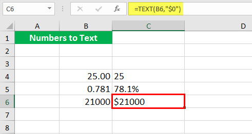
Suppose we have a number 21,000 in cell B6. We want to display the number as currency in the dollar.
To do this, we can use the TEXT Formula in ExcelTEXT function in excel is a string function used to change a given input to the text provided in a specified number format. It is used when we large data sets from multiple users and the formats are different.read more:
= TEXT (B6, “$0”)
It will return $21000.
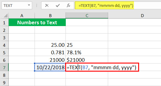
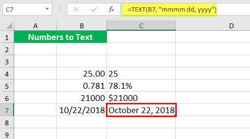
Suppose we have a date 10/22/2018 in cell B7, and we have to convert the date to another format.
We can use the TEXT formula:
= TEXT (B7, “mmmm dd, yyyy”)
It will return the date specified, i.e., October 22, 2018.
#2 Convert Numbers to Text using Excel Format Cell Option
Besides using the TEXT function, we can also use the format cell option to convert numbers to text in Excel.
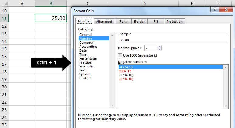
Suppose we have a number 25 in cell B11. We want to convert numbers to text.
To do so, we can press “CTRL + 1″(or COMMAND + 1 on Mac). As a result, a dialog box may appear, similar to the one shown below.
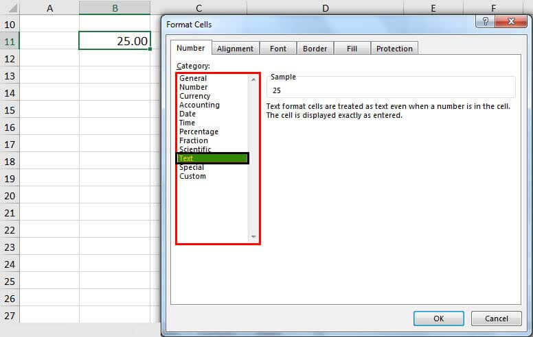
It mentions that the cell is currently formatted as a number. Now, we must select the “Text” option in the category.
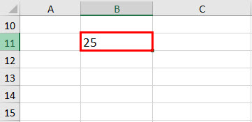
And click “OK.” We notice that the number has been formatted as “Text” now.
Similarly, we can change the formatting to a percentage, date, scientific notation in excelIn Excel, scientific notation is a specific style of writing numbers in scientific and exponential forms. Scientific notation compactly helps display values, allowing us to compare and use the same in calculations.read more, etc.
Suppose we want to convert cell B13 to percentage format.
We must select the cell and press “CTRL + 1” (or COMMAND + 1 for Mac) and select “Percentage.”
Then, click on “OK.”
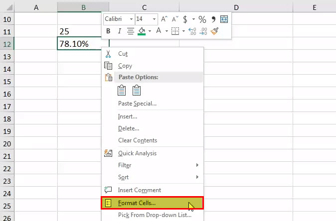
Instead of pressing “CTRL + 1” (or COMMAND + 1 in Mac), we can also right-click on the selected cell and then click on “Format Cells,” as shown below.
As shown in the above steps, we can select the “Text” option in the category and click “OK.”
Where can you Convert Numbers to Text in Excel?
Now, let us see some examples of converting numbers to text in Excel.
Example #1
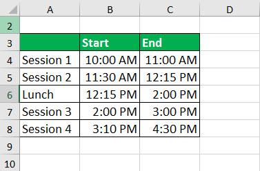
Suppose we have the start and end timings of different sessions held in the upcoming workshop organized by your company, as shown below. We are supposed to merge the two times, creating a range (time duration).
We first need to convert the time into “Text” format and then merge them to get a time range. For the first session, we can use the following TEXT formula:
= TEXT( B4, “hh:mm” ) & ( ” – ” ) & TEXT( C4, “hh:mm” ) & ( ” Hrs” )
It will return the time range for the 1st session.
Now, we can drag it to the rest of the cells to get the range for the rest of the cells.
Now, let us see the syntax in detail:
TEXT( B4, “hh:mm” ) & ( ” – ” ) & TEXT( C4, “hh:mm” ) & ( ” Hrs” )
TEXT( B4, “hh:mm”) will convert the given time in cell B4 to text in an hour: minute format (24 hours). Similarly, TEXT( C4, “hh:mm”) will convert the given time in cell C4 to an hour: minute format.
& (“-“) & will add “-” in between the two times, thus, creating a range.
& (“Hrs”) it will add the text Hrs at the end.
Similarly, we can also create a range of dates by modifying this syntax.
Example #2
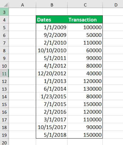
Suppose we have data for certain transactions accomplished in the past few years. Of those transactions, we want to know how many numbers of transactions were made during a particular month of a specific year and the total transaction amount. Therefore, the transaction data is given the cells B5: C19, as shown below.
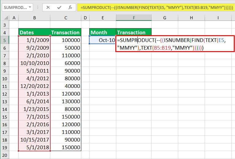
The month and year to look for are given in cell E5. To search the number of transactions held in the given month, we can use the SUMPRODUCT formula:
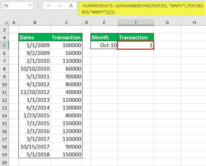
= SUMPRODUCT( –(( ISNUMBER ( FIND ( TEXT (E5, “MMYY”), TEXT ( B5:B19, “MMYY”))))))
And press the “Enter” key.
Now, to identify the total transaction amount during that period, we can use the following SUMPRODUCT FormulaThe SUMPRODUCT excel function multiplies the numbers of two or more arrays and sums up the resulting products.read more:
=SUMPRODUCT(– (EXACT( TEXT(E5, “mmyy”), TEXT( B5:B19, “mmyy”)) ), C5:C19)
It will return to 60000.
In both cases, the date given in cell E5 is first converted to “MMYY” format, and the dates given in cells B5:B19 are also converted to the same format and then matched. In the first case, wherever there is a match, it will return “TRUE” or “FALSE,” making an array. This array is then converted to numbers using ISNUMBERISNUMBER function in excel is an information function that checks if the referred cell value is numeric or non-numeric.read more, returning an array of 0 and 1. The SUMPRODUCT function will then count the number of 1 (i.e., TRUE, i.e., where we found the match), returning the number of transactions. The EXACT function will get the corresponding value wherever there is a match in the latter case. The SUMPRODUCT function will then sum the total transactions where we obtained a match.
Recommended Articles
This article is a guide to Convert Numbers to Text in Excel. Here, we discuss how to convert numbers using two methods – 1) Text Function and 2) Format Cell Options. Here, we also see case studies where we can convert numbers to text in Excel for appropriate usage, Excel examples, and downloadable Excel templates. You may also look at these useful functions in Excel: –
- Convert Function in Excel (Examples)As the word itself, the Excel CONVERT function defines that it can convert the numbers from one measurement system to another measurement system.read more
- How to Convert Excel to CSV?Converting Excel to CSV means converting data into text format by changing the file format to.txt. So, for the conversion, choose the required Excel file, click «Save As,» choose CSV as the format, and then save the file.read more
- Convert Date to Text in ExcelTo convert a date to text in Excel, right-click on the date cell and select the format cells option. A new window will open. You can convert the date to text by selecting the desired format from a list of options.read more
- Convert Columns to RowsThere are two ways to convert columns to rows: 1) using the Excel Ribbon Method. 2) The Mouse Method.read more


