Convert date formats excel - Word и Excel - помощь в работе с программами

Excel for Microsoft 365 Excel for the web Excel 2021 Excel 2019 Excel 2016 Excel 2013 Excel 2010 Excel 2007 More…Less

Occasionally, dates may become formatted and stored in cells as text. For example, you may have entered a date in a cell that was formatted as text, or the data might have been imported or pasted from an external data source as text.

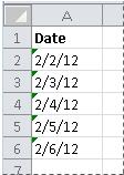
Dates that are formatted as text are left-aligned in a cell (instead of right-aligned). When Error Checking is enabled, text dates with two-digit years might also be marked with an error indicator: .

Because Error Checking in Excel can identify text-formatted dates with two-digit years, you can use the automatic correction options to convert them to date-formatted dates. You can use the DATEVALUE function to convert most other types of text dates to dates.

If you import data into Excel from another source, or if you enter dates with two-digit years into cells that were previously formatted as text, you may see a small green triangle in the upper-left corner of the cell. This error indicator tells you that the date is stored as text, as shown in this example.

You can use the Error Indicator to convert dates from text to date format.

Notes: First, ensure that Error Checking is enabled in Excel. To do that:

Click File > Options > Formulas.

In Excel 2007, click the Microsoft Office button , then click Excel Options > Formulas.
In Error Checking, check Enable background error checking. Any error that is found, will be marked with a triangle in the top-left corner of the cell.
Under Error checking rules, select Cells containing years represented as 2 digits.

Follow this procedure to convert the text-formatted date to a normal date:

On the worksheet, select any single cell or range of adjacent cells that has an error indicator in the upper-left corner. For more information, see Select cells, ranges, rows, or columns on a worksheet.

Tip: To cancel a selection of cells, click any cell on the worksheet.
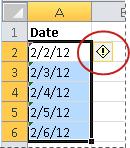
Click the error button that appears near the selected cell(s).
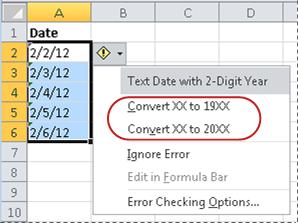
On the menu, click either Convert XX to 20XX or Convert XX to 19XX. If you want to dismiss the error indicator without converting the number, click Ignore Error.

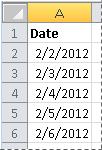
The text dates with two-digit years convert to standard dates with four-digit years.

Once you have converted the cells from text-formatted dates, you can change the way the dates appear in the cells by applying date formatting.

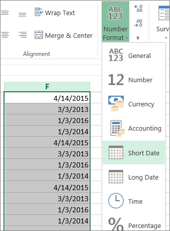
If your worksheet has dates that were perhaps imported or pasted that end up looking like a series of numbers like in the picture below, you probably would want to reformat them so they appear as either short or long dates. The date format will also be more useful if you want to filter, sort, or use it in date calculations.

Select the cell, cell range, or column that you want to reformat.
Click Number Format and pick the date format you want.

The Short Date format looks like this:

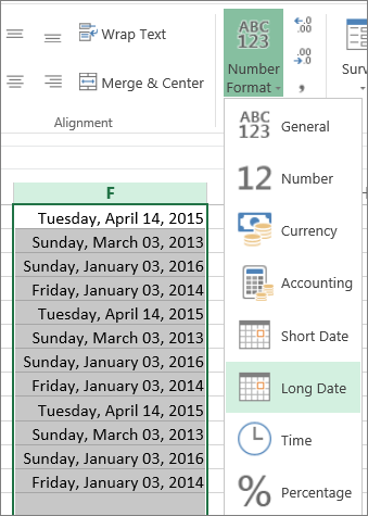
The Long Date includes more information like in this picture:

To convert a text date in a cell to a serial number, use the DATEVALUE function. Then copy the formula, select the cells that contain the text dates, and use Paste Special to apply a date format to them.

Follow these steps:

Select a blank cell and verify that its number format is General.
In the blank cell:
1. Enter =DATEVALUE(
2. Click the cell that contains the text-formatted date that you want to convert.
3. Enter )
4. Press ENTER, and the DATEVALUE function returns the serial number of the date that is represented by the text date.
  
  What is an Excel serial number?
  
  Excel stores dates as sequential serial numbers so that they can be used in calculations. By default, January 1, 1900, is serial number 1, and January 1, 2008, is serial number 39448 because it is 39,448 days after January 1, 1900.To copy the conversion formula into a range of contiguous cells, select the cell containing the formula that you entered, and then drag the fill handle across a range of empty cells that matches in size the range of cells that contain text dates.
After you drag the fill handle, you should have a range of cells with serial numbers that corresponds to the range of cells that contain text dates.
Select the cell or range of cells that contains the serial numbers, and then on the Home tab, in the Clipboard group, click Copy.

Keyboard shortcut: You can also press CTRL+C.
Select the cell or range of cells that contains the text dates, and then on the Home tab, in the Clipboard group, click the arrow below Paste, and then click Paste Special.
In the Paste Special dialog box, under Paste, select Values, and then click OK.
On the Home tab, click the popup window launcher next to Number.
In the Category box, click Date, and then click the date format that you want in the Type list.
To delete the serial numbers after all of the dates are converted successfully, select the cells that contain them, and then press DELETE.

Need more help?

You can always ask an expert in the Excel Tech Community or get support in the Answers community.

Need more help?

Want more options?

Explore subscription benefits, browse training courses, learn how to secure your device, and more.

Communities help you ask and answer questions, give feedback, and hear from experts with rich knowledge.

Источник

This post will guide you how to convert the current date to a specified date format in Excel. How do I convert date to YYYY-MM-DD format with Format Cells Feature in Excel. How to convert date format to a specific date format with a formula in Excel.

Convert Date to YYYY-MM-DD Format with Format Cell
Convert Date to YYYY-MM-DD Format with a Formula

Assuming that you have a list of data in range A1:A4, in which contain date values with MM/DD/YYYY format. And you need to convert the date to the YYYY-MM-DD format for your selected cells in Excel. How to do it. You can use achieve the result via format cells feature or a formula. Let’s see the following detailed introduction.

If you want to convert the selected range of cells to a given YYYY-MM-DD format, you can use the format cells to change the date format. Here are the steps:

#1 select the date values that you want to convert the date format.

convert date format yyyymmdd1

#2 right click on it, and select Format Cells from the pop up menu list. And the Format Cells will open.

convert date format yyyymmdd2

#3 switch to the Number tab in the Format Cells dialog box, and click the Custom category under the Category: list box, and enter the format code YYYY-MM-DD into the type text box, and click OK button.

convert date format yyyymmdd3

#4 the selected date values should be converted to YYYY-MM-DD format.

convert date format yyyymmdd4

Convert Date to YYYY-MM-DD Format with a Formula

You can also use an Excel formula based on the TEXT function to convert the given date value to a given format (yyyy-mm-dd). Like this:

=TEXT(A1,"yyyy-mm-dd")

Type this formula into a blank cell and press Enter key on your keyboard, and then drag the AutoFill Handle over to other cells to apply this formula.

convert date format yyyymmdd5

Источник

When you enter a date into Microsoft Excel, the program will format it according to the default date settings. For example, if you want to enter the date February 6, 2020, the date could appear as 6-Feb, February 6, 2020, 6 February, or 02/06/2020, all depending on your settings. You may find that if you change a cell’s formatting to “Standard,” your date becomes stored as integers. For example, February 6, 2020 would become 43865, because Excel bases date formatting off of January 1, 1900. Each of these options are ways to format dates in Excel. To help with organizing data in Excel, learn about how to change the date format in Excel.

Choosing from the Date Format List

Formatting dates in Excel is easiest with the date formats list. Most date formats you may want to use can be found in this menu.

How to Change The Excel Date Format

Select the cells you want to format
Click Ctrl+1 or Command+1
Select the “Numbers” tab
From the categories, choose “Date”
From the “Type” menu, select the date format you want

Creating a Custom Excel Date Format Option

To customize the date format, follow the steps for choosing an option from the date format list. Once you’ve selected the closest date format to what you want, you can customize it and change it.

In the “Category” menu, select “Custom”
The type you chose earlier will appear. The changes you make will only apply to your customized setting, not to the default
In the “Type” box, enter the correct code to alter the date
If you are trying to change the date display to DD/MM/YYYY, simply go to Format Cells > Custom
Next, Enter DD/MM/YYYY in the available space given.

Converting Date Formats to Other Locales

If you are using dates for several different locations, you might need to convert to a different locale:

Select the right cell or cells
Hit Ctrl+1 or Command+1
From the “Numbers” menu, select “Date”
Underneath the “Type” menu, there’s a drop-down menu for “Locale”
Select the right “Locale”

You can also customize the locale settings:

Follow the steps for customizing a date
Once you’ve created the right date format, you need to add the locale code to the front of the customized date format
Choose the right locale codes. All locale codes are formatted as [$-###]. Some examples include:
1. [$-409]—English, United States
2. [$-804]—Chinese, China
3. [$-807]—German, Switzerland
4. Find more locale codes

Tips for Displaying Dates in Excel

Once you have the right date format, there are additional tips to help you figure out how to organize data in Excel for your datasets.

Make sure the cell is wide enough to fit the entire date. If the cell isn’t wide enough, it will display #####. Double click on the right border of the column to make your column expand enough to display the date correctly.
Change the date system if negative numbers appear as dates. Sometimes Excel will format any negative numbers as a date because of the hyphens. To fix this, select the cells, open the options menu, and select “Advanced.” On that menu, select “Use 1904 date system.”
Use functions to work with today’s date. If you want a cell to always display the current date, use the formula =TODAY() and press ENTER.
Convert imported text to dates. If you import from an external database, Excel will automatically register the dates as text. The display may look the same as if they were formatted as dates, but Excel will treat the two differently. You can use the DATEVALUE function to convert.

Why Your Date Format May Not Be Having Issues Changing

There are many reasons why you might be experiencing issues changing the date format in Excel. Listed are a few common difficulties.

There could be text in the column, not dates (which are actually numbers).
Dates are left-aligned
An apostrophe could be included in the date
A cell may be too wide.
Negative numbers are formatted as dates
Excel TEXT function is not being utilized.

Even with correctly formatted dates and displays, organizing data in Excel can only work as well as the data does. Messy data won’t lead to insights during analysis, however, it’s formatted.

Data Preparation with Excel

Formatting data, by doing things like formatting dates, is part of a larger process known as “data preparation,” or all of the steps required to clean, standardize, and prepare data for analytic use.

While data preparation is certainly possible in Excel, it becomes exponentially more difficult as analysts work with larger and more complex datasets. Instead, many of today’s analysts are investing in modern data preparation platforms like Designer Cloud to accelerate the overall data preparation process for data big or small.

Schedule a demo of Designer Cloud to see how it can improve your data preparation process, or try the platform for yourself by getting started with Designer Cloud today.

Источник

In this guide, we’ll learn how to change date format in Excel. Date and Time data is an integral part of any statistical document or sheet. It is important to accurately track and analyze events, sales, figures, and others.

By convention, Excel uses a general data format that may be as per your need. But in most cases, that format may need to be customized.

Changing the format of Date in a particular cell or all the cells in your Excel sheet is an easy process and doesn’t require any complex methodologies. Excel provides a wide range of formatting options based on Location and Languages which helps in better date formatting in native language and style. Also, For some Languages there is also features to select from different Calendar types.

Follow the below step-by-step tutorial to change date format in Excel quickly and easily.

Step 1. Select the range of cells containing the date

To start with, select the cell values where want to change the date format, as shown in the image below.

Sample selection of dates in default formatting option

Step 2. Go to Number Format dropdown

To select ‘Number Format’, go to ‘Home‘ in the option menu and look for Number Format, as shown below
Then from the drop-down menu, select ‘More Number Formats‘ to reveal the ‘Number Format’ dialogue menu.

Select Number Format

Alternatively, you may directly go to Number Format, by right-clicking on the selected cell/s
Click on ‘Number Format’.

Right Click and select Number Format

Step 3. Choose Date

From the Category menu on the right, choose ‘Date‘.

Format Date option menu

Now, to apply any date formatting type, select it from the right panel of the pop-up menu of Number Format. Click on ‘OK‘ to apply the formatting to the selected cell/s.

Note: You may check the date format implementation in the ‘Sample‘ at the top of the menu option

Choose the Date Type

The general option type to choose from a variety of Date Formatting options. Scroll down in this section to reveal a plethora of options for formatting, ranging from date, text (month name), year, and others.

This option can be perceived as the display menu, as the formatting options in this will keep on changing as per the selection in Locale(Location) and Calendar type.

General Date Formatting

Choose the Locale (location)

This option features the Location or Language options to help format the date accordingly. This option is probably the most used option as users require to format the date according to their or audience preference as per the native formatting style, based on language and location.

Choose any language or Location from this options menu. After selecting, all the supported date format options available for that particular locale will be available for selecting in the above Type menu.

selecting locale (language) in date formatting

Choose the type of calendar

This option reveals different calendar types available based on the Locale(Location) selected from the above option menu. This formatting option is only available for certain Locale and not all.

As shown in our example below, the variety of calendar types available for selection are only available for the Locale (location) selected (here, Arabia), for other locales the calendar type might be different or not at all present.

Selecting Calendar type in Date Formatting

To apply selected formatting, you will need to click ‘OK‘ after selection to apply to your dates.

Conclusion

That’s It! You can now easily convert your dates to your desired format style easily.

We hope you learned and enjoyed this lesson and we’ll be back soon with another awesome Excel tutorial at QuickExcel!

Источник

Set yourself up

For a general overview of working with dates, see my previous article How to Convert Text Dates to Numeric.

The first step in analyzing data in Excel is typically to load a text file into the program. Frequently, this text file contains dates that we need for our analysis. It is important that Excel knows to treat this date text as dates because it has several functions that can make working with dates much simpler.

Excel is setup to recognize dates automatically in the short and long formats you use on Windows. In Windows 10, these are found and changed by going to Settings > Time & Language > Date & time > Change date and time formats.

A short date of d/MMM/yyyy means that the expected format is a day without a leading zero, followed by an abbreviated month name, and then a four digit year, with the three parts separated by “/”, as in “1/Jan/2001”. A long date of dddd, d MMMM yyyyy specifies the format as the day of the week, followed by a day without a leading zero, the full month name, and then the four-digit year, as in “Wednesday, 6/June/2018”. A short time of h:mm tt would be “5:30 pm”, and a long time of h:mm:ss tt “5:30:12 PM”.

Excel will recognize some additional common formats such as those involving numeric months with or without a leading 0 and yyyy-MM-dd (e.g., “2011-12-31”).

Analyze your date and time data

Built-in Functions for Manipulating Dates

In Excel 2016, you can find tools for working with dates by clicking “Date & Time” in the Formulas Ribbon.

The most important function for text date conversion in Excel is the DATEVALUE function. It is used to convert textual dates to a number that Excel recognizes as a date. The dates are stored as sequential numbers starting with 1 representing “Jan. 1, 1990”. For example, entering =DATEVALUE(“2011/02/23”) produces “40597”. The function TIMEVALUE similarly converts a textual time (“12:20 AM”) to a number that Excel recognizes as a time.

With the conversion accomplished, we can then either format the number into any date format we choose or use Excel’s special functions for working with dates. We can change the formatting by right clicking on the cell, selecting Format Cells and then selecting the desired format from the available date types.

If the desired format is not listed in the available types, we can also create a custom type by going to the Custom category and specifying the format, using the notation mentioned earlier: dd-mm-yy.

Excel provides functions to extract parts of a date such as DAY, YEAR, and WEEKDAY. Other useful functions include NOW to get the current date and time, and DAYS to compute the number of days between two dates.

Analyze your date and time data

Conversion with Non-Standard Formats

Unfortunately, if your dates are in a more complex or less common format, Excel may not be able to recognize them right away. We’ll have to add an additional step to convert the dates to a recognized format. We can resort to extracting parts of the text string using the functions LEFT, MID, and RIGHT and then combine the pieces using & or CONCATENATE into a format that Excel supports. For example, if my text string is “2018-Feb-02”, which Excel does not recognize, I can use the following formula to swap the positions of the day and year parts of the text to become “02-Feb-2018”, which Excel does recognize.

=RIGHT(A2,2)&»-«&MID(A2,6,3)&»-«&LEFT(A2,4)

You can quickly analyze your data and time data in Displayr. Get started below.

Источник