
A contingency table (sometimes called “crosstabs”) is a type of table that summarizes the relationship between two categorical variables.
Fortunately it’s easy to create a contingency table for variables in Excel by using the pivot table function. This tutorial shows an example of how to do so.
Example: Contingency Table in Excel
Suppose we have the following dataset that shows information for 20 different product orders, including the type of product purchased (TV, computer, or radio) along with the country (A, B, or C) that the product was purchased in:

Use the following steps to create a contingency table for this dataset:
Step 1: Select the PivotTable option.
Click the Insert tab, then click PivotTable.

In the window that pops up, choose A1:C21 for the range of values. Then choose a location to place the pivot table in. We’ll choose cell E2 within the existing worksheet:

Once you click OK, an empty contingency table will appear in cell E2.

Step 2: Populate the contingency table.
In the window that appears on the right, drag Country into the box titled Rows, drag Product into the box titled Columns, and drag Order Number into the box titled Values:

Note: If Values first appears as “Sum of Order Number” simply click the dropdown arrow and select Value Field Settings. Then choose Count and click OK.
Once you do so, the frequency values will automatically be populated in the contingency table:

Step 3: Interpret the contingency table.
The way to interpret the values in the table is as follows:
Row Totals:
- A total of 4 orders were made from country A.
- A total of 8 orders were made from country B.
- A total of 8 orders were made from country C.
Column Totals:
- A total of 6 computers were purchased.
- A total of 5 radios were purchased.
- A total of 9 TV’s were purchased.
Individual Cells:
- A total of 1 computer was purchased from country A.
- A total of 3 computers were purchased from country B.
- A total of 2 computers were purchased from country C.
- A total of 0 radios were purchased from country A.
- A total of 2 radios were purchased from country B.
- A total of 3 radios were purchased from country C.
- A total of 3 TV’s were purchased from country A.
- A total of 3 TV’s were purchased from country B.
- A total of 3 TV’s were purchased from country C.
Additional Resources
How to Create a Contingency Table in R
How to Create a Contingency Table in Python
A contingency table, also known as a crosstab is used to show the relationship between two categorical variables. In excel, we can make a contingency table using the pivot table function. They are best for summarizing the relationship between categorical variables. A Contingency table is just like a frequency distribution table in which we can show two variables simultaneously. To further derive results from a Contingency table, chi-square tests are used. In this article, we will learn how to create a Contingency Table.
Creating a Contingency Table
Let us take the following dataset and convert it into a contingency table. This dataset consists of product IDs, product names, and the product manufacturer. The dataset that you want to convert into a contingency table can have any number of rows or columns. T

Follow the following steps to create the contingency table from this dataset.
Step 1: Choose the PivotTable option from the Insert tab. This will open a dialog box.

Step 2: In the dialog box that appears, choose the range of values as $A1:$C6 and then choose another cell in the sheet where you want to place the pivot table. Here, we have chosen cell G1. The range of values is the entire space that contains the dataset.

Step 3: Now click ok and you will see an empty contingency table in the G1 cell. It appears in the G1 cell because that was what we choose in the location in Step 2.

Step 4: Now, we have to populate the table. In other words, we have to fill this empty table with the dataset values. But, we do not have to do this manually. In the window on the left, drag Manufacturer into the box named Rows, drag Names into the box named Columns, and drag Id in the box named Values.

Notice that the frequency values are automatically populated in the contingency table. This is the required contingency table for the dataset assumed above.

Now when we have successfully created the contingency table, let us see how we can read it to derive useful information from it.
Interpretation of the Contingency table
One of the major advantages of using a Contingency table is that it makes the visualization of the relationship between variables very easy. We can interpret a Contingency table based on rows, columns as well as cells.
Based on row total
- 2 products are made by manufacturer X.
- 1 product is made by manufacturer Y.
- 2 products are made by manufacturer Z.
Based on column total
- Milk sold was 1.
- Soya sold were 2.
- Tofu sold was 2.
Based on individual cells
- 2 Tofus were purchased from Manufacturer X.
- 1 Milk was purchased from Manufacturer Y.
- 2 Soyas were purchased from Manufacturer Z.
This tutorial shows how to create a cross-tab, also called contingency table from two qualitative variables in Excel using the XLSTAT software.
Dataset to create a cross-tab or contingency table
The dataset contains information on 20 clients: their age, city of residence and gender. We will create a contingency table based on the Age and City variables.
Creating a cross-tab or contingency table
After opening XLSTAT, select the XLSTAT / Preparing data / Create a contingency table command.

Once you’ve clicked on the relevant button, the dialog box appears.
In the General tab, select the category variable you wish to use in rows. Select the Age variable by selecting the entire column. Then select the variable to be used in columns. Here we choose the City variable. The columns B and C contain variable labels so the option Variable labels should be ticked.
You may activate the By group analysis field if you want to use a layer variable, such as the gender, and generate a three-way cross-tab.

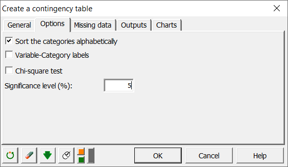
In the Options tab, you can decide how the categories of the variable should be treated. Also you can choose to run a Chi-square test. In this case, however, we will only select the Sort the categories alphabetically option.
In the Outputs tab, select the Contingency table as well as the observed and theoritical frequencies.

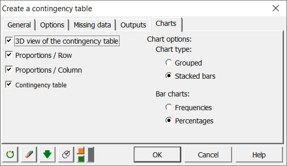
Select the following options in the tab Charts.
The computations begin once you have clicked on the OK button, and the results are displayed on a new sheet.
Results of the creation of a cross-tab or contingency table
The first result is the contingency table. Notice that clients are absent in certain crossed categories. For example there is no detected client in Paris of age class 25-34.

The next output is the 3-D plot followed by a stacked bar chart, which is a good visualization of the data distribution.


Next are the two tables containing the frequencies Age/City. You can compare the actual distribution of the clients and the theoritical distribution if the distribution was random.

Statistical tests on cross-tabs or contingency tables
It is possible to test if the two qualitative variables that shape the contingency table are independent.
Advantages of using XLSTAT cross-tabs instead of Excel pivot tables
Among the many advantages of using the XLSTAT contingency table feature compared to Excel pivot tables: — XLSTAT is able to automatically output test results on the contingency tables.
-
You can enter as many qualitative variables as you want in both the row and column variable fields in XLSTAT. XLSTAT will produce one result for each possible pair of row/column variables.
The following video tackles crosstabs with an illustration using XLSTAT:

Was this article useful?
- Yes
- No
Contingency tables are commonly used in statistics. Let’s learn how to do a contingency table in Microsoft Excel.
Contingency tables are commonly used in statistics. In essence, they measure frequency distributions of multiple variables. They’re a quick visual way to count frequencies in an intuitive way. Fortunately, they’re easy to build with spreadsheets. Let’s learn how to do a contingency table in Microsoft Excel.
Imagine that you’re a sales manager, and you want to track product sales by color, by region. A contingency table is the perfect way to do it. Begin by building out a quick layout in an Excel spreadsheet like the one below.
As you can see, the purchase order numbers are listed in column A. The regions are in column B, and the color of the products are in column C. To add a contingency table, you can convert this simple layout into a pivot table.
To do so, click and drag to select the range of data. Here, the range is A1:C8. Then, go to the Insert tab on Excel’s ribbon. On the Insert tab, click PivotTable over on the left side.

On the Create PivotTable menu, click Existing Worksheet, then click into cell A10 in the Table/Range box. Then, click OK. Excel will add your PivotTable.

On the PivotTable Fields box, move Region into the Rows box. Color goes in the Columns box, and PO #Number goes in the Values box. It will default to Sum, but you can click on the i icon and choose Count instead.

Just like that, you’ve created a contingency table in Excel. At a glance, you can tell how many products were sold by color, by region. Plus, the PivotTable automatically calculates totals for both colors and regions. This is a great fast way to perform a visual statistical analysis on your data. Try it out next time you need to build tables quickly.
Recommended tutorials:
Calculate Percentage in Excel
Formula Builder in Excel


Excel is a great app you can use whenever you’re working with data.
You can perform various mathematical, scientific, or even statistical equations with it.
Excel has tons of formulas, functions, and features that can help you with that.
One of the more complex things you can do with Excel is data analysis.
Excel has many tools that can assist its users in analyzing data.
Among these is the creation of pivot tables.
These nifty tables/charts help with summarizing and reorganizing selected columns and rows.
As a result, you’ll obtain reports about the selected data (e.g. frequency of a particular variable, a list of unique values, etc.).
Note that pivot tables don’t change the dataset itself. Rather, they only show a different perspective of the selected data.
With the create pivot table tool in Excel, you can create a Contingency table (a.k.a. crosstab).
It is usually used to show the relationship between two categorical variables.
Generally, a Contingency table displays the frequency of particular variables.
And it does so in a table or matrix format, which makes it easier to read and digest for the user.
You can even further derive results from a Contingency table using chi-square tests.
Because of the insight that a Contingency table provides, it is widely used in research sectors such as scientific research, statistics, survey research, etc.
Create a Contingency Table in Excel
In this article, I’ll be showing you how you can create a Contingency table in Excel.
By the end of the article, you should be able to create a Contingency table whenever you need to.
Let’s get started.
Use the Insert PivotTable Button to Create a Contingency Table in Excel
The more popular method of creating a Contingency table in Excel involves inserting a pivot table in Excel.
To do so, you’ll have to click on the Insert PivotTable button.
This button can be accessed by opening the Insert tab. On the very left side of the ribbon, you’ll see the PivotTable button (or as how I would call it, the Insert PivotTable button).

Clicking on the dropdown arrow below the button will allow you to create a pivot table from one of three sources: (1) From Table/Range (default option), (2) From External Data Source, and (3) From Data Model.

Clicking on the button itself will create a Pivot table based on the selected Table or Range of Cells.
Now, let’s proceed to how we can use this button to create a contingency table in Excel.
How to Create a Contingency Table
To create a Contingency table, we must first have a dataset to base on.
And so, we’ll be using the following dataset for illustration:

From this data set, we want to get the following data: (1) the number of teams, (2) the total number of players per team, (3) the number of male and female players per team, (4) the total number of male and female players, and (5) the total number of players.
To do so, we’ll create a Contingency table.
Insert PivotTable
- Select the table or range of cells which you want to derive the Contingency table from. Make sure to include the column headers in the selection. In our illustration, we’ll be selecting cells A1:C16.

- Click on the Insert PivotTable button. To do so, open the Insert tab. On the very left side of the ribbon, you’ll see the PivotTable button. Click on it.
- Since we’ve already selected the data from which we’ll derive the Contingency table, the textbox next to Table/Range should already be filled up.

- Next, we’ll have to select where we want our Contingency table to appear: (1) on a new worksheet, or (2) on the same worksheet as the source data. For our illustration, we’ll be selecting the 2nd option which is on the same worksheet as the source data.

- Lastly, we’ll have to select where on the worksheet should the Contingency table appear. Click on the textbox next to Location. Then, select the first cell of the Contingency table (an easy way to do this is to click on the cell). For our illustration, this will be cell A18.

- (Optional) To analyze multiple tables, check the box next to “Add this data to the Data Model”.
- Click the OK button. This should open the PivotTable Fields dialog box.


Creating the Contingency Table
We’ll now have to set the pivot table to make it into a contingency table. To do so, we’ll have to drag the variable to their respective areas.

- For our illustration, we’ll be dragging the variable to these areas: Team -> Rows, Gender -> Columns, and Player ID –> Values.

- Next, we’ll have to change the Sum of Player ID in the values into the Count of Player ID. To do so, click on Sum of Player ID. This will show you a list of options. Select Value Field Settings from among them.

- In the box below “Summarize value field by”, select count. This should summarize the variably by count (i.e. frequency). Click the OK button after doing so.

- And there we have it. We have successfully created a contingency table.

Interpreting the Contingency Table
Now that we have our Contingency Table, let’s see if we can finally obtain our desired data
The number of teams
We can get this data by counting the number of rows which is 3. These three teams are Blue, Red, and Yellow.

The total number of players per team
We can get this by looking at the grand total per row (team). Each team (Blue, Red, and Yellow) has 5 players.

The number of male and female players per team
We can get this by taking a look at where the Team and Gender Columns meet. Blue team has 4 female members and 1 male member. Red team has 0 female members and 5 male members. Yellow team has 3 female member and 2 male members.

The total number of male and female players
We can get this by looking at the total per column. There are 7 female players and 8 male players.

The total number of players
We can get this by looking at the grand total, which is 15.

Conclusion
And that’s how you create a Contingency table in Excel.
While it can be intimidating at first, it’s not really that hard once you get to know how to use the Insert PivotTable tool to create a Contingency table.
I hope that you’re able to learn something from this article.
Contents
- 1 What is a cross tabulation called in Excel?
- 2 What is crosstab format?
- 3 Is cross tabulation Chi Square?
- 4 Is a crosstab the same as a pivot table?
- 5 How do you transpose in Excel?
- 6 Why do we use crosstabs?
- 7 What is contingency in Excel?
- 8 What is relative contingency table?
- 9 What is a two way contingency table?
- 10 What is the difference between crosstabs and Chi Square?
- 11 How does a crosstabs with chi square analysis function?
- 12 Is Chi square and crosstab the same?
- 13 What does a contingency table display?
- 14 What is Panda crosstab?
- 15 How do you make a panda crosstab?
- 16 How do I traverse data in Excel?
- 17 How do you do transposition?
- 18 What is preserved in a csv file?
- 19 Which tabulation is all example of cross-tabulation?
- 20 What is a row vs column?
What is a cross tabulation called in Excel?
Cross tabulation is a method to quantitatively analyze the relationship between multiple variables. Also known as contingency tables or cross tabs, cross tabulation groups variables to understand the correlation between different variables.
What is crosstab format?
The Crosstab format is one of the most popular. Crosstab stands for Cross tabulation, a process by which totals and other calculations are performed based on common values found in a set of data. In Microsoft Excel™ the term “Pivot Table” is used for a Crosstab.Each sale is represented by a row of data.
Is cross tabulation Chi Square?
Crosstabulation is a powerful technique that helps you to describe the relationships between categorical (nominal or ordinal) variables.
Is a crosstab the same as a pivot table?
The Differences Between Pivot Tables and Crosstabs
Pivot tables and crosstabs are nearly identical in form, and the terms are often used interchangeably. However, pivot tables present some added benefits that regular crosstabs do not.
How do you transpose in Excel?
TRANSPOSE function
- Step 1: Select blank cells. First select some blank cells.
- Step 2: Type =TRANSPOSE( With those blank cells still selected, type: =TRANSPOSE(
- Step 3: Type the range of the original cells. Now type the range of the cells you want to transpose.
- Step 4: Finally, press CTRL+SHIFT+ENTER.
Why do we use crosstabs?
Crosstabs in SPSS is just another name for contingency tables, which summarize the relationship between different variables of categorical data. Crosstabs can help you show the proportion of cases in subgroups.
What is contingency in Excel?
A contingency table (sometimes called “crosstabs”) is a type of table that summarizes the relationship between two categorical variables. Fortunately it’s easy to create a contingency table for variables in Excel by using the pivot table function.
What is relative contingency table?
In a contingency table (sometimes called a two way frequency table or crosstabs), conditional relative frequency is it’s a fraction that tells you how many members of of a group have a particular characteristic.
What is a two way contingency table?
2 that a two-way contingency table is a display of counts for two categorical variables in which the rows represented one variable and the columns represent a second variable. The starting point for analyzing the relationship between two categorical variables is to create a two-way contingency table.
What is the difference between crosstabs and Chi Square?
Cross tabulation table (also known as contingency or crosstab table) is generated for each distinct value of a layer variable (optional) and contains counts and percentages. Chi-square test is used to check if the results of a cross tabulation are statistically significant.
How does a crosstabs with chi square analysis function?
A cross tabulation displays the joint frequency of data values based on two or more categorical variables. The joint frequency data can be analyzed with the chi-square statistic to evaluate whether the variables are associated or independent.This table shows frequency counts for each production line and shift.
Is Chi square and crosstab the same?
Crosstabulation is a statistical technique used to display a breakdown of the data by these two variables (that is, it is a table that has displays the frequency of different majors broken down by gender). The Pearson chi-square test essentially tells us whether the results of a crosstab are statistically significant.
What does a contingency table display?
In statistics, a contingency table (also known as a cross tabulation or crosstab) is a type of table in a matrix format that displays the (multivariate) frequency distribution of the variables.They provide a basic picture of the interrelation between two variables and can help find interactions between them.
What is Panda crosstab?
Pandas crosstab() , the basics
crosstab() function takes two or more lists, pandas series or dataframe columns and returns a frequency of each combination by default.Cross tabulation just means taking one variable, displaying its groups as indexes, and taking the other, displaying its groups as columns.
How do you make a panda crosstab?
Start the Process
- import pandas as pd import seaborn as sns.
- pd. crosstab(df. make, df. body_style)
- df. groupby([‘make’, ‘body_style’])[‘body_style’]. count(). unstack(). fillna(0)
- df. pivot_table(index=’make’, columns=’body_style’, aggfunc={‘body_style’:len}, fill_value=0)
How do I traverse data in Excel?
Start by selecting and copying your entire data range. Click on a new location in your sheet, then go to Edit | Paste Special and select the Transpose check box, as shown in Figure B. Click OK, and Excel will transpose the column and row labels and data, as shown in Figure C.
How do you do transposition?
There are four steps to transposition:
- Choose your transposition.
- Use the correct key signature.
- Move all the notes the correct interval.
- Take care with your accidentals.
What is preserved in a csv file?
CSV (Comma delimited)
This file format (. csv) saves only the text and values as they are displayed in cells of the active worksheet. All rows and all characters in each cell are saved. Columns of data are separated by commas, and each row of data ends in a carriage return.
Which tabulation is all example of cross-tabulation?
Cross tabulation is a statistical tool that is used to analyze categorical data. Categorical data is data or variables that are separated into different categories that are mutually exclusive from one another. An example of categorical data is eye color.
What is a row vs column?
What is the Difference between Rows and Columns?
| Rows | Columns |
|---|---|
| A row can be defined as an order in which objects are placed alongside or horizontally | A column can be defined as a vertical division of objects on the basis of category |
| The arrangement runs from left to right | The arrangement runs from top to bottom |