
Excel для Microsoft 365 Excel для Microsoft 365 для Mac Excel для Интернета Excel 2021 Excel 2021 для Mac Excel 2019 Excel 2019 для Mac Excel 2016 Excel 2016 для Mac Еще…Меньше
Функция CONCAT объединяет текст из нескольких диапазонов и (или) строк, но не предоставляет аргументы delimiter или IgnoreEmpty.
Функция CONCAT заменяет функцию CONCATENATE. Функция СЦЕПИТЬ (CONCATENATE) также будет поддерживаться для совместимости с более ранними версиями Excel.
Синтаксис
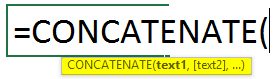
СЦЕПИТЬ(текст1; [текст2]; …)
|
Аргумент |
Описание |
|---|---|
|
text1 |
Элемент текста, который нужно присоединить. Строка или массив строк, например диапазон ячеек. |
|
[text2, …] |
Дополнительные текстовые элементы для объединения. Для текстовых элементов можно указать до 253 аргументов. Каждый из них может быть строкой или массивом строк, например диапазоном ячеек. |
Например, выражение =СЦЕП(«Не»;» «;»слышны»;» «;»в»;» «;»саду»;» «;»даже»;» «;»шорохи.») вернет строку Не слышны в саду даже шорохи.
Совет: Чтобы включить разделители (например, интервалы или амперсанды (&)) между текстом, который требуется объединить, и удалить пустые аргументы, которые не должны отображаться в объединенном текстовом результате, можно использовать функцию TEXTJOIN.
Примечания
-
Если объединенная строка содержит свыше 32767 символов (ограничение для ячейки), функция СЦЕП вернет ошибку #ЗНАЧ!.
Примеры
Скопируйте данные примеров из приведенных ниже таблиц и вставьте их в ячейку A1 нового листа Excel. Чтобы отобразить результаты формул, выделите их и нажмите клавишу F2, а затем — клавишу ВВОД. При необходимости измените ширину столбцов, чтобы видеть все данные.
Пример 1
|
=СЦЕПИТЬ(B:B; C:C) |
A’s |
B’s |
|---|---|---|
|
a1 |
b1 |
|
|
a2 |
b2 |
|
|
a4 |
b4 |
|
|
a5 |
b5 |
|
|
a6 |
b6 |
|
|
a7 |
b7 |
Так как эта функция допускает ссылки на целый столбец и строку, она возвращает следующий результат: A’sa1a2a4a5a6a7B’sb1b2b4b5b6b7
Пример 2
|
=СЦЕПИТЬ(B2:C8) |
A’s |
B’s |
|---|---|---|
|
a1 |
b1 |
|
|
a2 |
b2 |
|
|
a4 |
b4 |
|
|
a5 |
b5 |
|
|
a6 |
b6 |
|
|
a7 |
b7 |
Результат: a1b1a2b2a4b4a5b5a6b6a7b7
Пример 3
|
Данные |
Имя |
Фамилия |
|---|---|---|
|
вида |
Виталий |
Токарев |
|
речная форель |
Fourth |
Pine |
|
32 |
||
|
Формула |
Описание |
Результат |
|
=СЦЕПИТЬ(«Популяция рек для «;A2;» «;A3;» составляет «;A4;» на километр.») |
Создает предложение, объединяя данные в столбце А с остальным текстом. |
Популяция рек для вида речная форель составляет 32 на километр. |
|
=СЦЕПИТЬ(B2;» «; C2) |
Объединяет строку в ячейке В2, пробел и значение в ячейке С2. |
Виталий Токарев |
|
=СЦЕПИТЬ(C2; «, «; B2) |
Объединяет текст в ячейке C2, строку, состоящую из запятой и пробела, и значение в ячейке B2. |
Токарев, Виталий |
|
=СЦЕПИТЬ(B3;» & «; C3) |
Объединяет строку в ячейке B3, строку, состоящую из пробела, амперсанда и еще одного пробела, и значение в ячейке C3. |
Fourth & Pine |
|
=B3 & » & » & C3 |
Объединяет те же элементы, что и в предыдущем примере, но с помощью оператора & (амперсанд) вместо функции СЦЕПИТЬ. |
Fourth & Pine |
Дополнительные сведения
Вы всегда можете задать вопрос специалисту Excel Tech Community или попросить помощи в сообществе Answers community.
См. также
Функция СЦЕПИТЬ
Функция ОБЪЕДИНИТЬ
Общие сведения о формулах в Excel
Рекомендации, позволяющие избежать появления неработающих формул
Поиск ошибок в формулах
Сочетания клавиш и горячие клавиши в Excel
Текстовые функции (справочник)
Функции Excel (по алфавиту)
Функции Excel (по категориям)
Нужна дополнительная помощь?

When dealing with Excel workbooks, data may be structured in a way that doesn’t fit your needs and objectives.
Sometimes, you may need to split the content of one cell into different cells. You may also need to do the opposite, combining data from multiple columns into one.
The second process is called concatenation. Most often, you use concatenation in Excel to join such data as names and addresses, display time, and date.
In this guide, we will look at concatenation in detail and examine the techniques that you can use in different situations.
What Does “Concatenate” Mean?
Generally, Excel enables you to combine data in two ways: you can either merge cells or concatenate their values.
The first option means turning multiple cells into one. As a result, you get a single large cell that is displayed across multiple columns or rows.
If you choose to concatenate cells instead, you won’t merge the cells themselves but combine their content.
Concatenation doesn’t impact cells but joins multiple values. For example, you can use this method to combine pieces of textual content from different cells. In Excel, such content is called text strings. You can also insert a number obtained from a formula in-between textual content.
For example, you may have your customers’ first names in column B, and their last names in column C. You may want column D to contain both their first and last names, but retyping their names manually is too time-consuming and inefficient.
In this case, you can use concatenation functions, like “CONCATENATE,” “CONCAT,” and “&.” Let’s consider each one of these formulas and figure out the differences.
CONCATENATE
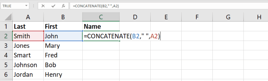
Excel lets you to join text strings in different ways. First of all, you can use the CONCATENATE function. In this case, your formula will look like this:
=CONCATENATE(X1,X2,X3)
X1, X2, and X3 are the cells that you want to join.
If you want to separate values of cells with spaces, you can add them in quotation marks, separated with commas:
=CONCATENATE(X1,“ ”,X2)
CONCAT
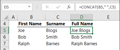
CONCATENATE is the oldest function of this kind and the only function you can use to join text strings when dealing with Excel 2013.
However, if you’re using a newer version of Excel, you might consider updated functions. The CONCATENATE function may also be unavailable in future versions. The CONCAT function works with Excel 2016 and Excel Mobile.
You can use this formula in the same way as CONCATENATE, but CONCAT is certainly easier to use because it’s shorter.
Here’s what the example above would look like with the CONCAT function:
=CONCAT(X1,X2,X3)
The “&” Operator

However, you may also choose not to use either of the formulas above and choose an even simpler option — the ampersand operator (&). This method of joining cells is recommended by Microsoft, and it’s much easier to use than the CONCAT and CONCATENATE functions.
Here’s an example of a formula that you can use:
=X1&X2&X3
If you want to separate the values of cells with spaces or commas, here’s what your formulae will look like:
=X1&“ ”&X2
=X1&“,”&X2
Using the “&” operator is a more convenient option. Besides, the “&” operator has no limitations regarding the number of strings that you can join.
In contrast, the CONCATENATE function is limited to 8,192 characters, which means that you can only use it to join up to 255 strings. However, sometimes you may want to use the CONCAT function to keep your formulae clean and to make them easier to read.
TEXTJOIN
Another function that you can use when combining textual content is TEXTJOIN. This function only works with the latest versions of Microsoft Office, and it offers some nice features.
First, you can choose how you want to separate the values of different cells, with no need to type these spaces, commas, or other symbols in the formula.
Secondly, the TEXTJOIN function enables you to ignore empty cells while including an array of arguments.
Here’s what the TEXTJOIN function looks like in Excel:
=TEXTJOIN(delimiter,ignore_empty,text1,[text2],…)
“Delimiter” is the separator that you want to use between different text strings, and “ignore_empty” can only take two values: TRUE or FALSE.
When using TEXTJOIN, you can still add cells manually, but in this case, the “&” operator would be a better choice. TEXTJOIN enables you to add a whole range of cells.
For example, here’s what function you can use to join text strings from the range A1:A4, separated with commas, ignoring empty values:
=TEXTJOIN(“,”,TRUE,A1:A4)
If you want to separate text strings with spaces and include empty values, the formula will look like this:
=TEXTJOIN(“ ”,FALSE,A1:A4)
How to Concatenate Text Strings With Line Breaks
Most often, Excel users need to separate text strings with spaces and punctuation marks. In this case, you can use formulae from the previous sections, depending on the chosen functions or operators.
However, sometimes you may need to separate text strings with a carriage return, or line break. For example, you may need to merge data and mailing addresses from separate columns or rows.
Unfortunately, you cannot put line breaks in formulae as easily as you do with punctuation marks because they are not regular characters. The good news is that you can include virtually any characters you want by using ASCII codes.
In this case, you should use the CHAR function. To include a line break on Windows, you should use CHAR(10), because 10 is the ASCII code for a line feed. On Mac, you should use CHAR(13), since 13 is the ASCII code for carriage return.
Keep in mind that you should also enable the “Wrap text” option to display the result correctly. Press Ctrl+1, then choose the “Alignment” tab in the “Format Cells” menu and then check the “Wrap text” box.
How to Concatenate Columns
To concatenate multiple columns, you can write a regular concatenation formula in the first cell, and then drag the fill handle to copy it to other cells.
To do it quickly, you can select the cell that contains the necessary formula, and then double-click the fill handle. Excel decides how far cells should be copied after your double click based on which cells are present in your formula. Therefore, if your table contains empty cells, you may need to drag the fill handle manually.
How to Concatenate a Range of Cells
Given that the CONCATENATE and CONCAT functions only accept single-cell references in arguments, joining values from multiple cells can be a challenge.
To quickly select multiple cells, you can press Ctrl and then click on each of the cells that you want to combine.
However, if you’re dealing with too many cells, this method may also be too time-consuming. In this case, you can use the TRANSPOSE function, which looks like this:
=TRANSPOSE(X1:Xn)
Type the TRANSPOSE formula in a cell where you want to include the concatenated range, then click on the formula bar, and press F9 to replace your formula with concatenated values. After this, you should delete the curly braces around the array values, type =CONCAT( before the first value, and add a closing parenthesis after the last value.
Things to Keep in Mind about Concatenating
Don’t forget to put commas between the concatenated items. For example, if you want to get the phrase “write my research paper,” your formula should be =CONCAT(“write”,“ ”,”my”,“ ”,”research”,“ ”,“paper”).
In this example, all items are also separated with designated spaces. You can also include extra spaces after each text string to avoid typing them separately in formulae.
If you type =CONCAT(“Hi”“there”), without a comma, the result will look like this: Hi”there. An extra quotation mark will appear because there’s no comma between the arguments.
If you see the “#NAME?” error instead of the desired result, it likely means that you forgot to include some quotation marks. The “#VALUE!” error means that some of the arguments are invalid.
You should also keep in mind that concatenate functions always return a text string, even if some cells contain numerical values. You can also convert numbers to text by using the TEXT function and use different formulae to set the format of numbers that you want to combine with text or symbols.
For example, if your A2 cell contains the number 13.6 and you want to display it as a dollar amount, your formula should be =TEXT(A2,“$0.00”). As a result, you will get $13.60.
Wrapping Up
Excel lets you to join text strings by using different functions, such as CONCATENATE, CONCAT, and the “&” operator.
While you can only use the CONCATENATE function in Excel 2013, the newer versions of Excel support a simple “&” operator that is much easier to use.
When concatenating values of different cells, pay attention to quotation marks and commas because they are very important for displaying the results properly.
I hope that this guide will help you save a lot of time and make your workflow as efficient as possible.
Learn to code for free. freeCodeCamp’s open source curriculum has helped more than 40,000 people get jobs as developers. Get started
Russian (Pусский) translation by Andrey Rybin (you can also view the original English article)
Многие люди воспринимают Microsoft Excel, как инструмент по работе с электронными таблицами. Хотя Excel используется для модификации и создания электронных таблиц, его особая функция — это автоматизация работы с данными.
Одним из ключевых навыков для работы с данными является объединение ячеек, также известное как конкатенация. Давайте рассмотрим способы объединения данных в Microsoft Excel.
Что Означает Конкатенация?
Предположим, что у вас есть имя клиента в колонке С, и фамилия в колонке D. Вы хотите, чтобы в колонке E, у вас было записано полное имя, состоящее из этих двух частей, но это слишком затратно, заново все записывать в новой колонке.
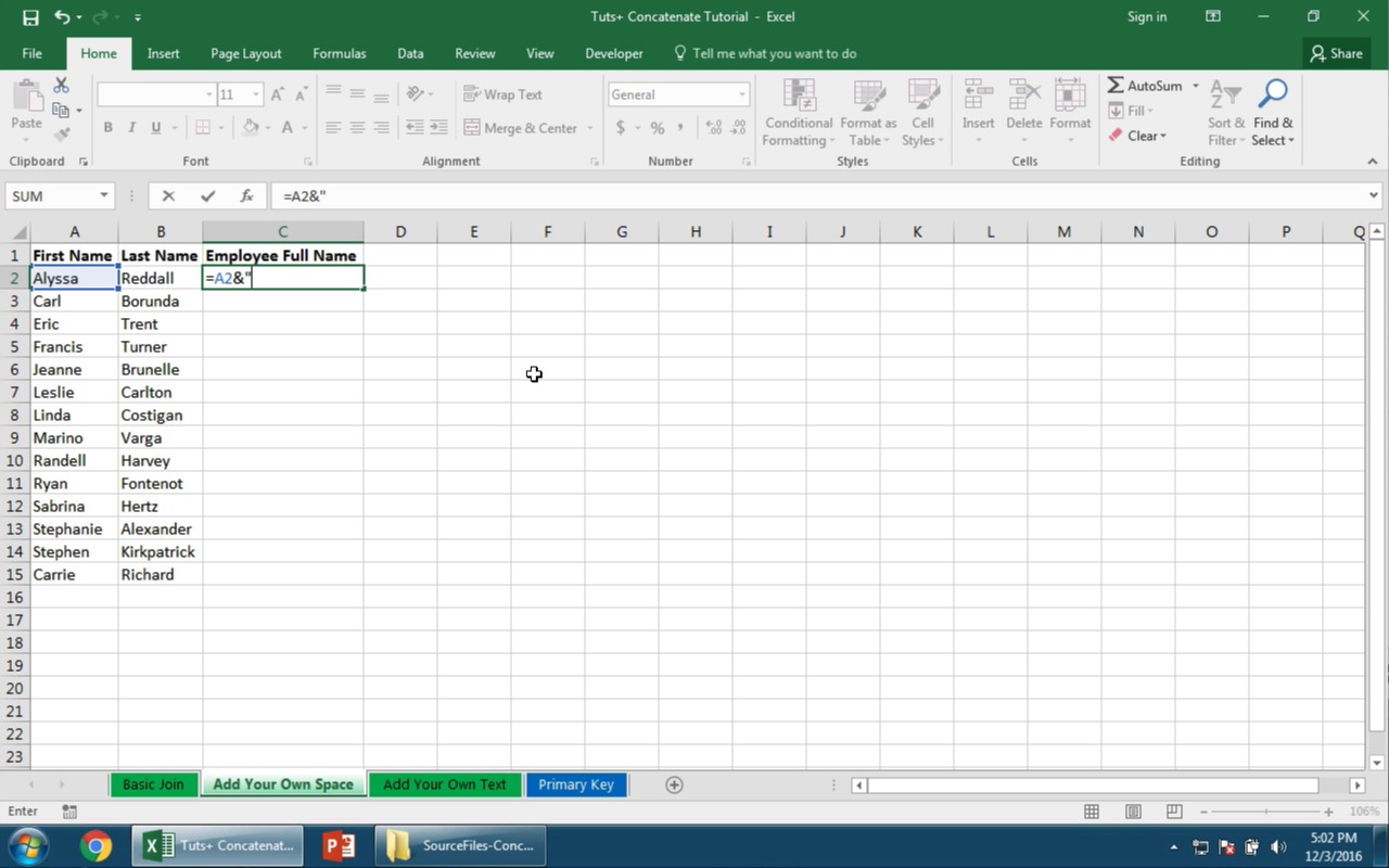
На рисунке ниже я работаю с данными о сотрудниках. У меня есть имя и фамилия в разных колонках, но я хочу объединить их в одно полное имя в колонке E.


К счастью, Excel может сделать это для нас автоматически. Эта техника называется конкатенация, и в общем под этим подразумевается объединение ячеек.
На скриншоте выше, я использовал простую конкатенацию чтобы объединить имя и фамилию сотрудников, и пробел между ними, чтобы получить полное имя. Продолжайте читать, чтобы узнать как это сделать:
Как Делать Конкатенацию в Excel (Смотри и Учись)
Посмотрите этот короткий видеоурок ниже, чтобы получить представление о том, как использовать конкатенацию для объединения текстовых строк и данных. И обязательно закачайте бесплатное приложение к уроку в виде рабочих документов Excel. А затем прочтите текстовую часть урока, чтобы узнать еще больше о конкатенации в Microsoft Excel.
3 Способа Объединения Текста в Excel
Excel обычно предоставляет нам различные способы, чтобы сделать какую-то одну вещь, и объединение ячеек здесь не исключение. Есть простой способ сделать это, но я думаю, что важно знать все способы, чтобы понять таблицу, которая досталась вам от кого-то еще.
1. СЦЕПИТЬ
Используется в Excel 2013 и более ранних версиях
= СЦЕПИТЬ(А1;А2;А3)
Вы можете использовать функцию СЦЕПИТЬ, чтобы объединять ячейки. Используйте точку с запятой, чтобы разделять ячейки или поля, которые вы хотите объединить. Однако, если вы пользуетесь Excel 2016, то возможно вы захотите использовать более обновленную версию этой функции, о которой расскажем дальше.
2. СЦЕП
Используется в Excel 2016 и Excel Mobile.
=СЦЕП(A1;A2;A3)
В Excel 2016 Microsoft отказались от функции СЦЕПИТЬ и заменила ее на СЦЕП (прим. перевод.: однако поддержка старой функции так же осталось, для возможности работы с документами старых версий). Использование точно такое же, просто Microsoft сократили название. (Кто же будет их обвинять? Я часто ошибаюсь в длинном названии).
Если вы открываете электронную таблицу в Excel 2013 или более поздней версии, она по-прежнему работает правильно в Excel. Со временем вы возможно обновите свои формулы и будете использовать СЦЕП, но есть третий способ объединять ячейки, который я рекомендую использовать прежде вего. Давайте узнаем, про этот способ.
3. «&»
Рекомендуемый способ объединения текста.
=A1&A2&A3
Корпорация Майкрософт рекомендует использовать простой & оператор, в качестве способа объединения ячеек. На самом деле, это действительно легче, чем печатать любую из предыдущих функций. Просто вставьте «&» между ссылками на ячейки, чтобы объединить их в одну новую строку.
Однако, иногда может быть сложно прочитать формулу с «&» стоящей между каждой парой ячеек, или прочесть кусок текста в формуле. Чтобы формула лучше читалась, я могу использовать СЦЕП. Любая функция отлично работает для объединения.
3 Практических Упражнения по Объединениям в Excel
Для всех этих примеров я буду использовать рекомендуемый для объединения текста & оператор . Давайте рассмотрим примеры.
Для этих упражнений, я рекомендую использовать документы Excel, которые я создал специально для этого урока. Если вы пропустили это раньше, то обязательно скачайте бесплатно прилагающиеся к этому уроку, Книгу Excel, с которой вы сможете работать и следить за действиями по ходу урока.
Упражнение 1. Элементарное объединение в Excel
Используйте вкладку с названием Basic Join в книге Excel прилагающейся к этому уроку.
Давайте начнем с простого примера по объединению текста. В этом примере, я собираюсь комбинировать пары из простых слов, чтобы составить сложное слово, например «barn» и «yard» чтобы получить barnyard.
Для этого мы используем самый простой подход. Чтобы объединить текст из ячейки А2 с текстом в ячейке В2, я записал простую формулу в ячейке С2:
=A2&B2


Excel объединит текст из ячеек А2 и В2 и в результате получится сложное слово в С2. Я могу потянуть формулу вниз, чтобы распространить ее и на другие ячейки, чтобы комбинировать все данные из колонок А и В.
Упражнение 2. Добавление Пробела в Объединение
Используйте вкладку с названием Add Your Own Space из Excel — книги, прилагающейся к уроку.
Ранее, я приводил классический пример конкатенации: объединение имени и фамилии, чтобы получить полное имя. Это идеальный вариант для использования конкатенации, потому что переименовывать все этих имена обременительно и является пустой тратой времени.
Однако, нам надо немного изменить формулу. Если мы объединим мое имя и фамилию, то мы получим «AndrewChildress«. Нам нужно вставить пробел в формулу, чтоб разделить имя и фамилию. Давайте посмотрим, как это сделать:
В этом примере, я собираюсь объединить ячейки С2 и D2 (колонки, те что слева на картинке). И еще, нам нужно вставить пробел, между именем и фамилией.
Мы можем использовать кавычки, чтобы добавить наш собсвтенный текст в объединение. Просто используйте еще одни символ «&», и пробел внутри, чтобы разделить имя. Посмотрите, как это должно выглядеть:


Кавычки с пробелом внутри разделяют имя на две части, и мы получаем нормальную запись. Вот как выглядит моя окончательная формула:
=C2&" "&D2
Упражнение 3. Добавление Вашего Текста
Используйте вкладку с названием Add Your Own Text из Excel — книги, прилагающейся к уроку.
Теперь, давайте в процессе объединения добавим текст. Принцип такой же как и с пробелом, нам нужно вставить свой текст в кавычки.
Среди данных на картинке ниже, у меня есть колонка А с пунктом назначения. Я хочу, чтобы в колонке В, было сообщение «I’ve been to«(я был в), и затем название из колонки А. Проблема в том, что у меня нет «I’ve been to» в моей таблице, поэтому я вручную вбиваю это в формулу.
На картинке ниже, я написал формулу, в которой объединяется имя города с моей приветственной фразой.


Не забудьте добавить точку в конце, чтобы получилось правильное предложение! Я написал строковую переменную в кавычках — («I’ve been to «) и затем добавил A2, и добавил точку в конце.
В результате моя формула выглядит следующим образом:
="I've been to "&A2&"."
Продвинутый Уровень Excel: Создание Первичного Ключа
Давайте поднимемся на уровень выше, к более теоретическим концепциям. Если вы используете таблицу в виде базы данных с важной информацией, то каждая запись (строка) в вашей базе данных должна иметь первичный ключ.
Первичный ключ, позволяет вам уникальным образом идентифицировать вашу строку и отличить ее от других. Подходящей областью, для использования такой концепции, может быть база данных заказов клиентов. Важно, чтобы мы сгенерировали такой первичный ключ, для которого не будет повторений в других записях.


Проблема в том: как нам узнать, нет ли у нас повторений? Нам нужно сгенерировать первичный ключ, чтобы уникальным образом идентифицировать транзакции.
Ниже несколько пояснений, почему плохо использовать одну колонку в виде первичного ключа:
- Мы не можем использовать имя клиента, чтобы уникальным образом идентифицировать транзакцию. Что если у нас будет два покупателя с именем «Боб Смит»?
- Мы не можем использовать время заказа в качестве уникального идентификатора. В большом магазние, в одно время могут быть зарегестрированы две покупки.
- Также и наименование товара, заказанного клиентом или адрес доставки, могут появляться несколько раз в вашей базе данных.
В общем, ни одна из колонок, о которых я говорил выше, не подходит для уникальной идентификации. Но если мы объединим все колонки вместе, мы увеличим вероятность того, что значение будет абсолютно уникальным.
В примере показаном выше, я дал вариант, как можно выполнить конкатенацию колонок, чтобы создать первичный ключ. В общем-то, все что я делаю, это объединяю вместе все колонки:
=A2&B2&C2&D2&E2&F2&G2
В результате получается мешанина символов в колонке H. Однако, это как раз то, что нам нужно.


Теперь, у каждой транзакции есть свой уникальный идентификатор. Мы избавились от любых конфликтов имен или почтовых адресов, или адресов доставки, объединив вместе несколько колонок.
Вы можете запустить функцию Удалить Дубликаты для колонки H, чтобы вычистить любые конфликтующие записи. Вы также можете эффективно использовать функцию ВПР, потому, что строки уникальны.
Есть много приложений, для которых может понадобиться первичный ключ. Здесь важно использовать интегральую характеристику ваших записей, чтобы сделать каждую транзакцию или строку уникальной.
Подводим Итоги и Продолжаем Обучение
СЦЕП и «&» — казалось бы, просты формулы Excel, но они гораздо ценнее, чем может показаться на первый взгляд. Не важно просто ли вы объединяете данны в более сложные строки, или создаете первичный ключ, я думаю, что это хороший навык, которому стоит научиться.
- Наш другой урок Как Находить и Удалять Дубликаты — это урок Excel, в котором мы рассматриваем автоматизацию повседневной работы по очистке данных.
- Официальная документация Microsoft по СЦЕП и СЦЕПИТЬ — это ценный и авторитетный источник, из которого можно во всех подробностях узнать как объединять текст и ячейки.
- Я начал этот урок с того, что назвал Excel отличным инструментом автоматизации. ВПР — это другая функция, которая позволяет автоматизировать работу с данными и избежать перепечатывания данных, и по этой функции у нас также есть урок — как использовать ВПР.
Может вы можете придумать другие примеры использования этой функции и поделитесь этим с читателями Envato Tuts+? Оставляйте комментарии ниже, делитесь своими знаниями или задавайте вопросы.
Excel Concatenate Strings (Table of Contents)
- Introduction to Concatenate Strings in Excel
- How to Use Concatenate Strings in Excel?
Introduction to Concatenate Strings in Excel
Concatenate in Excel is used to combine values from several cells in one cell or join different pieces of text in one cell. This function is mostly used where data is not structured in excel and where we want to combine the data of two or more columns in one column or a row. Concatenate is very helpful in structuring the data according to our requirements. It combines strings and text together and is a built-in function in excel. Concatenate is replaced as CONCAT from Excel 2016 and newer versions. It is known as the Text/String function as well.
Concatenate can join up to 30 text items and combine them to make one text.
Syntax:
How to Use Concatenate Strings in Excel?
There are multiple ways to use the concatenate function. We will take a look at them with the help of some formulas.
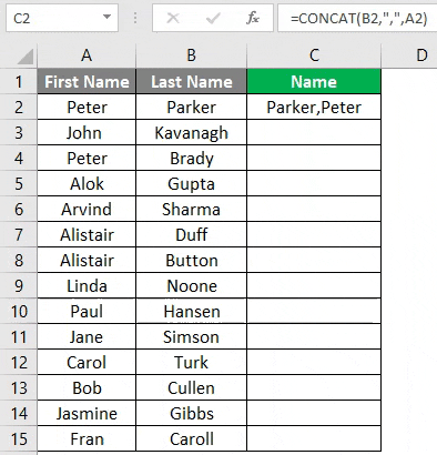
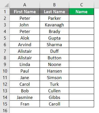
Let’s see an example below where we need to join the first and last names of employees by using concatenate function.
You can download this Concatenate Strings Excel Template here – Concatenate Strings Excel Template
Example #1 – CONCATENATE using Formula Tab in Excel
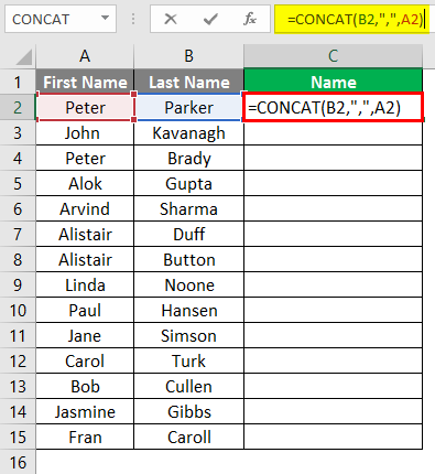
In the below image, we have two columns of first and last name.
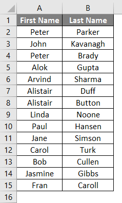
Now we would join their first and last name to get the complete name by using concatenate function. Let’s see the steps to insert the Concatenate Function to Join the First and Last Name.
Go to Column C2.

Select Formulas Icon and click on Insert Function as shown below.
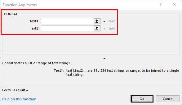
Then select a Category as “TEXT” and then select the Function category will open in which you can select CONCAT Function and Click OK.
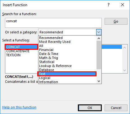
A window will open, as shown below after clicking OK, where you can type the text you want to concatenate.
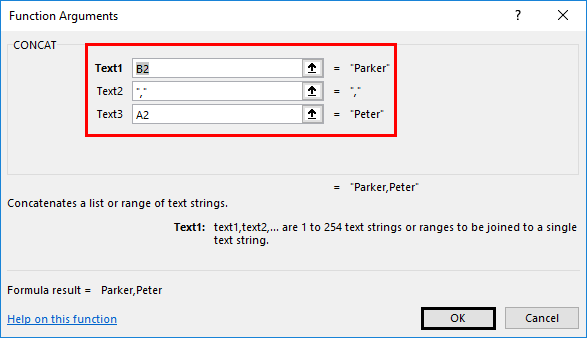
For column C2, in-text 1 gives reference to cell B2, which is the Last Name, Text 2-Put Comma inside semicolons and in Text 3, reference to cell B1, which is the first name.
Click on the OK button.
The last name followed by the first name will be concatenated in column C2.
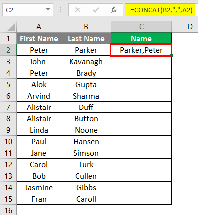
Drag down the formula till the end of the data, and the formula will be applied for the rest of the data.
Example #2 – CONCATENATE Using Direct Formula
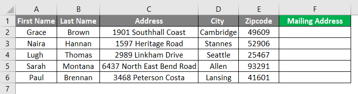
As you can see in the below screenshot, we need to concatenate the text in Column A (First Name), Column B (Last Name), Column C (Address), Column D (City) and column E(Zipcode) to arrive at the Mailing address in Column F.
We can do this by simply entering the function in cell F6.
Steps for Entering the Concatenate Function
- Type “=CONCATENATE(“ in cell H6.
- Now give the reference of cell B6 for Text1.
- Enter space in between the semicolons for Text2.
- Give the reference of cell C6 for Text3.
- Enter comma”,” in-between the semicolons for Text4.
- Give the reference of cell D6 for Text5.
- Enter comma”,” in-between the semicolons for Text6.
- Give the reference of cell E6 for Text7.
- Enter dash”-” in between the semicolons for Text8.
- Give the reference of cell F6 for Text9.
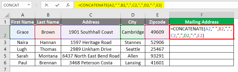
Press Enter Key after entering the formula.
Drag down the formula in the below cells to get the mailing address details of other rows.
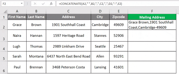
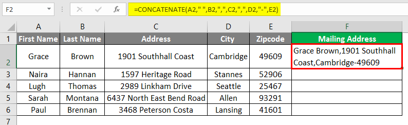
As you can see in the above screenshot, we have the mailing address in column H for all the persons.
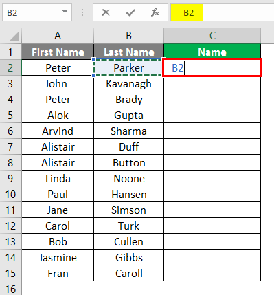
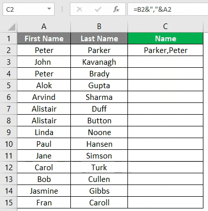
Example #3 – CONCATENATE Using “&” Operator
The way to concatenate is by using the “&” operator instead of concatenate function. Let us take the same example that we used in Example 1, where we want to join the first name and the last name.
To concatenate the text strings in column A and B with the help of the “&” operator, all we need to do is to follow the below steps. Go to cell C2 and give cell reference of cell B2, as shown in the below screenshot.
Now Insert “&” operator and comma and space in between the semicolons”, “as shown in the below screenshot.
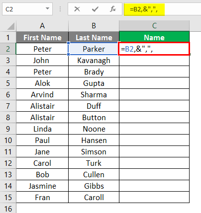
Now again, Insert the “&” operator and give the reference of cell A2 and close the bracket.
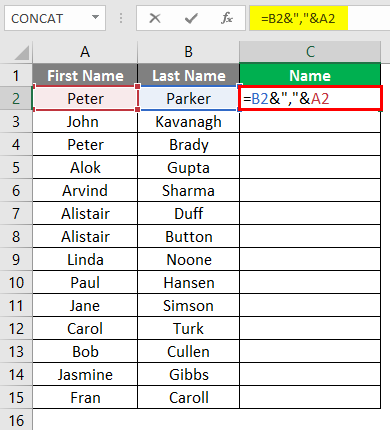
Press the Enter Key, and you will get the desired result.
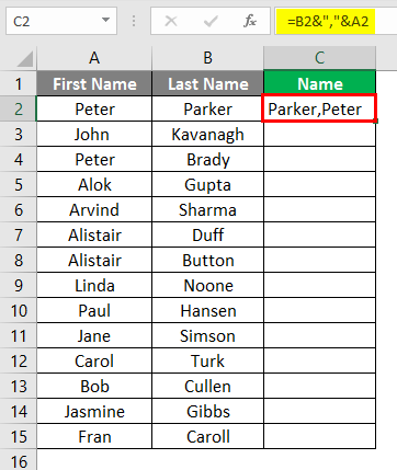
Drag the formula till the end of the data.
Example #4 – CONCATENATE Using Calculated Field
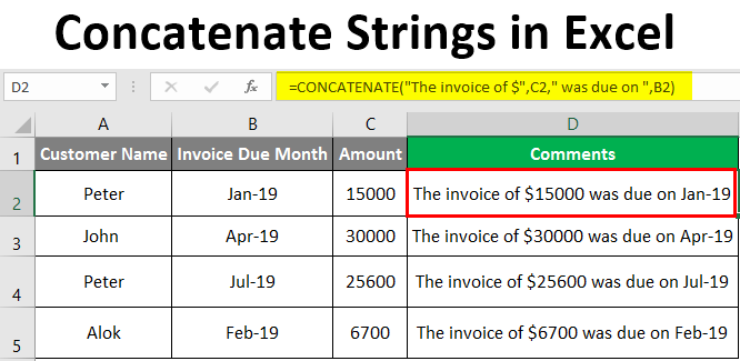
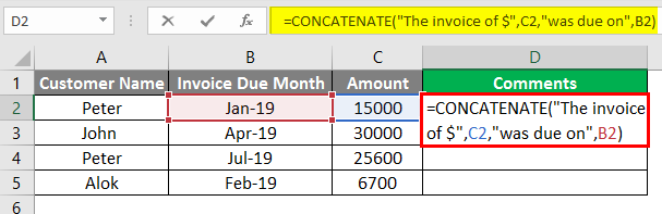
We can concatenate the text string even by calculating a certain field. Suppose you have the data of a few customers, and you need to enter certain comments for those customers, as given in the below screenshots.
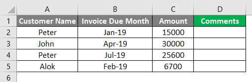
The comment we need in column D is like this “The invoice of certain $ value was due on this Month”. To get such comments in column D, we need to follow the below steps. Go to cell D2 and Enter CONCATENATE function as below.
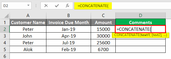
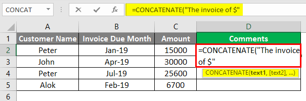
Now Insert the Comment “The invoice of $” in between the semicolon as Text1.
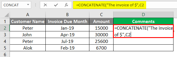
Now give the reference of cell C2, which is the invoice amount value for Text2.
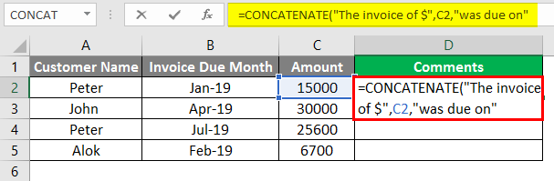
Give the comment “was due on” with one space in between the semicolon as Text3.
Give the cell reference of cell B2, which is the invoice due Month as Text4. Close the bracket.
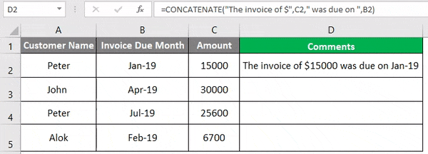
Press the Enter key, and You can see the final comment in cell D2 as below.
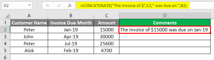
Drag down the formula for the rest of the data.
Things to Remember About Concatenate Strings in Excel
- Concatenate function requires at least one argument to work.
- From Excel 2016 or Newer Version, CONCATENATE is replaced with the CONCAT. The Concatenate function will still work as it is still kept for backward compatibility. However, we don’t it will be kept in future versions, so it is highly recommendable to use CONCAT instead of CONCATENATE.
- The result of the concatenate function is always a Text String. Even if you use numbers to concatenate, the result will always be in the form of a text string.
- In Concatenate, each cell reference needs to be listed separately; it doesn’t recognize arrays.
- In CONCATENATE Function, you can use 8192 characters which means you can concatenate up to 255 Strings.
- The formula will give #Value! Error if anyone’s argument is invalid.
- The difference between the concatenate function and using the “&” operator to concatenate text string is that there is no limitation of 255 strings while using the “&” operator. Apart from that, there is no difference.
Recommended Articles
This is a guide to Concatenate Strings in Excel. Here we discuss how to use concatenate strings in Excel along with practical examples and a downloadable excel template. You can also go through our other suggested articles to learn more–
- Concatenation in Excel
- Opposite of Concatenate in Excel
- VBA Concatenate Strings
- Excel Concatenate Date

This Excel tutorial explains how to use the Excel & operator with syntax and examples.
Description
To concatenate multiple strings into a single string in Microsoft Excel, you can use the & operator to separate the string values.
The & operator can be used as a worksheet function (WS) and a VBA function (VBA) in Excel. As a worksheet function, the & operator can be entered as part of a formula in a cell of a worksheet. As a VBA function, you can use this operator in macro code that is entered through the Microsoft Visual Basic Editor.
Syntax
The syntax for the & operator is:
string1 & string2 [& string3 & string_n]
Parameters or Arguments
- string1, string2, string3, … string_n
- The string values to concatenate together.
Returns
The & operator returns a string/text value.
Applies To
- Excel for Office 365, Excel 2019, Excel 2016, Excel 2013, Excel 2011 for Mac, Excel 2010, Excel 2007, Excel 2003, Excel XP, Excel 2000
Type of Function
- Worksheet function (WS)
- VBA function (VBA)
Example (as Worksheet Function)
Let’s look at some Excel & operator examples and explore hwo you would use the & operator as a worksheet function in Microsoft Excel:
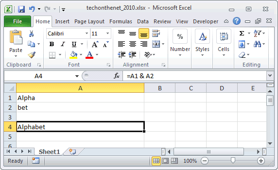
Based on the Excel spreadsheet above, the following & examples would return:
=A1 & A2
Result: "Alphabet"

="Tech on the " & "Net"
Result: "Tech on the Net"

=(A1 & "bet soup")
Result: "Alphabet soup"
Concatenate Space Characters
When you are concatenating values together, you might want to add space characters to separate your concatenated values. Otherwise, you might get a long string with the concatenated values running together. This makes it very difficult to read the results.
Let’s look at an easy example.
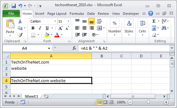
Based on the Excel spreadsheet above, we can concatenate a space character using the & operator as follows:
=A1 & " " & A2
Result: "TechOnTheNet.com website"
In this example, we have used the & operator to add a space character between the values in cell A1 and cell A2. This will prevent our values from being squished together.
Instead our result would appear as follows:
"TechOnTheNet.com website"
Here, we have concatenated the values from the two cells (A1 and A2), separated by a space character.
Concatenate Quotation Marks
Since the & operator will concatenate string values that are enclosed in quotation marks, it isn’t straight forward how to add a quotation mark character to the concatenated results.
Let’s look at a fairly easy example that shows how to add a quotation mark to the resulting concatenated string using the & operator.
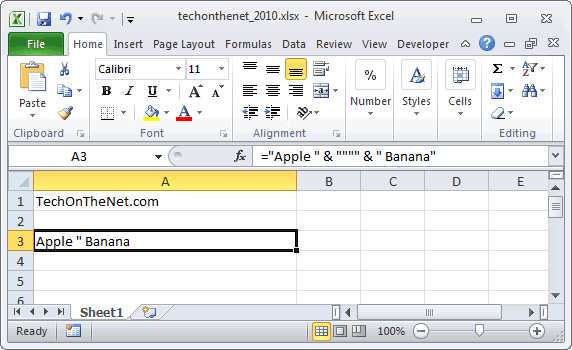
Based on the Excel spreadsheet above, we can concatenate a quotation mark as follows:
="Apple " & """" & " Banana"
Result: Apple " Banana
In this example, we have used the & operator to add a quotation mark to the middle of the resulting string.
Since our strings to concatenate are enclosed in quotation marks, we use 2 additional quotation marks within the surrounding quotation marks to represent a quotation mark in our result as follows:
""""
Then when you put the whole function call together:
="Apple " & """" & " Banana"
You will get the following result:
Apple " Banana
Frequently Asked Questions
Question:For an IF statement in Excel, I want to combine text and a value.
For example, I want to put an equation for work hours and pay. If I am paid more than I should be, I want it to read how many hours I owe my boss. But if I work more than I am paid for, I want it to read what my boss owes me (hours*Pay per Hour).
I tried the following:
=IF(A2<0,"I owe boss" abs(A2) "Hours","Boss owes me" abs(A2)*15 "dollars")
Is it possible or do I have to do it in 2 separate cells? (one for text and one for the value)
Answer: There are two ways that you can concatenate text and values. The first is by using the & character to concatenate:
=IF(A2<0,"I owe boss " & ABS(A2) & " Hours","Boss owes me " & ABS(A2)*15 & " dollars")
Or the second method is to use the CONCATENATE function:
=IF(A2<0,CONCATENATE("I owe boss ", ABS(A2)," Hours"), CONCATENATE("Boss owes me ", ABS(A2)*15, " dollars"))
Example (as VBA Function)
Let’s look at some Excel & operator function examples and explore how to use the & operator in Excel VBA code:
The & operator can be used to concatenate strings in VBA code. For example:
Dim LValue As String

LValue = "Alpha" & "bet"
The variable LValue would now contain the value «Alphabet».
Frequently Asked Questions
Question:For an IF statement in Excel, I want to combine text and a value.
For example, I want to put an equation for work hours and pay. If I am paid more than I should be, I want it to read how many hours I owe my boss. But if I work more than I am paid for, I want it to read what my boss owes me (hours*Pay per Hour).
I tried the following:
=IF(A2<0,"I owe boss" abs(A2) "Hours","Boss owes me" abs(A2)*15 "dollars")
Is it possible or do I have to do it in 2 separate cells? (one for text and one for the value)
Answer: There are two ways that you can concatenate text and values. The first is by using the & character to concatenate:
=IF(A2<0,"I owe boss " & ABS(A2) & " Hours","Boss owes me " & ABS(A2)*15 & " dollars")
Or the second method is to use the CONCATENATE function:
=IF(A2<0,CONCATENATE("I owe boss ", ABS(A2)," Hours"), CONCATENATE("Boss owes me ", ABS(A2)*15, " dollars"))