Concat cells in excel

Combine text from two or more cells into one cell

You can combine data from multiple cells into a single cell using the Ampersand symbol (&) or the CONCAT function.

Combine data with the Ampersand symbol (&)

1. Select the cell where you want to put the combined data.

2. Type = and select the first cell you want to combine.

3. Type & and use quotation marks with a space enclosed.

4. Select the next cell you want to combine and press enter. An example formula might be =A2&» «&B2.

Combine data using the CONCAT function

1. Select the cell where you want to put the combined data.

2. Type =CONCAT(.

3. Select the cell you want to combine first.

   Use commas to separate the cells you are combining and use quotation marks to add spaces, commas, or other text.

4. Close the formula with a parenthesis and press Enter. An example formula might be =CONCAT(A2, » Family»).

Need more help?

See also

TEXTJOIN function

CONCAT function

Merge and unmerge cells

CONCATENATE function

How to avoid broken formulas

Automatically number rows

Combining values with CONCATENATE is the best way, but with this function, it’s not possible to refer to an entire range.

You need to select all the cells of a range one by one, and if you try to refer to an entire range, it will return the text from the first cell.

In this situation, you do need a method where you can refer to an entire range of cells to combine them in a single cell.

So today in this post, I’d like to share with you 5 different ways to combine text from a range into a single cell.

[CONCATENATE + TRANSPOSE] to Combine Values

The best way to combine text from different cells into one cell is by using the transpose function with concatenating function.

Look at the below range of cells where you have a text but every word is in a different cell and you want to get it all in one cell.

Below are the steps you need to follow to combine values from this range of cells into one cell.

1. In the B8 (edit the cell using F2), insert the following formula, and do not press enter.
   • =CONCATENATE(TRANSPOSE(A1:A5)&” “)
2. Now, select the entire inside portion of the concatenate function and press F9. It will convert it into an array.
3. After that, remove the curly brackets from the start and the end of the array.
4. In the end, hit enter.

That’s all.

How this formula works

In this formula, you have used TRANSPOSE and space in the CONCATENATE. When you convert that reference into hard values it returns an array.

In this array, you have the text from each cell and a space between them and when you hit enter, it combines all of them.

Combine Text using the Fill Justify Option

Fill justify is one of the unused but most powerful tools in Excel. And, whenever you need to combine text from different cells you can use it.

The best thing is, that you need a single click to merge text. Have look at the below data and follow the steps.

1. First of all, make sure to increase the width of the column where you have text.
2. After that, select all the cells.
3. In the end, go to Home Tab ➜ Editing ➜ Fill ➜ Justify.

This will merge text from all the cells into the first cell of the selection.

TEXTJOIN Function for CONCATENATE Values

If you are using Excel 2016 (Office 365), there is a function called “TextJoin”. It can make it easy for you to combine text from different cells into a single cell.

Syntax:

TEXTJOIN(delimiter, ignore_empty, text1, [text2], …)

1. delimiter a text string to use as a delimiter.
2. ignore_empty true to ignore blank cell, false to not.
3. text1 text to combine.
4. [text2] text to combine optional.

how to use it

To combine the below list of values you can use the formula:

=TEXTJOIN(" ",TRUE,A1:A5)

Here you have used space as a delimiter, TRUE to ignore blank cells and the entire range in a single argument. In the end, hit enter and you’ll get all the text in a single cell.

Combine Text with Power Query

Power Query is a fantastic tool and I love it. Make sure to check out this (Excel Power Query Tutorial). You can also use it to combine text from a list in a single cell. Below are the steps.

1. Select the range of cells and click on “From table” in data tab.
   
2. If will edit your data into Power Query editor.
   
3. Now from here, select the column and go to “Transform Tab”.
4. From “Transform” tab, go to Table and click on “Transpose”.
   
5. For this, select all the columns (select first column, press and hold shift key, click on the last column) and press right click and then select “Merge”.
   
6. After that, from Merge window, select space as a separator and name the column.
   
7. In the end, click OK and click on “Close and Load”.

Now you have a new worksheet in your workbook with all the text in a single cell. The best thing about using Power Query is you don’t need to do this setup again and again.

When you update the old list with a new value you need to refresh your query and it will add that new value to the cell.

VBA Code to Combine Values

If you want to use a macro code to combine text from different cells then I have something for you. With this code, you can combine text in no time. All you need to do is, select the range of cells where you have the text and run this code.

 Sub combineText()
 Dim rng As Range
 Dim i As String
 For Each rng In Selection
 i = i & rng & " "
 Next rng
 Range("B1").Value = Trim(i)
 End Sub 

Make sure to specify your desired location in the code where you want to combine the text.

In the end,

There may be different situations for you where you need to concatenate a range of cells into a single cell. And that’s why we have these different methods.

All methods are easy and quick, you need to select the right method as per your need. I must say that give a try to all the methods once and tell me:

Which one is your favorite and worked for you?

Please share your views with me in the comment section. I’d love to hear from you, and please, don’t forget to share this post with your friends, I am sure they will appreciate it.

Combine Data in Cells Using the CONCATENATE Operator or Functions

by Avantix Learning Team | Updated February 20, 2022

Applies to: Microsoft^® Excel^® 2013, 2016, 2019, 2021 and 365 (Windows)

You can combine the data from multiple cells into another cell using the CONCATENATE operator or CONCATENATE functions. CONCATENATE is often used to combine text in cells (like first name and last name) but you can also combine text with numbers, dates, functions, spaces, commas or dashes. If you have Excel 2019 or a later version, you can also use the CONCAT function. It is important to note that combining cells is different from merging cells.

Recommended article: How to Merge Cells in Excel (4 Ways)

Do you want to learn more about Excel? Check out our virtual classroom or in-person Excel courses >

In this article, we’ll look at 3 ways to combine cells using CONCATENATE:

• Using the CONCATENATE operator
• Using the CONCATENATE function
• Using the CONCAT function

If you want to combine dashes, commas, spaces or other text in an expression with CONCATENATE, you need to enter it in quotation marks or double quotes (such as » «).

If you want to enter formulas in an Excel table, you can use structured reference formulas which must refer to fields in square brackets []. You would also need to precede the field name with @ to refer to the current record.

Combining cells using the CONCATENATE operator (&)

You can use the CONCATENATE operator (&) to combine cells into one cell using a formula. Using the CONCATENATE operator, you can combine multiple cells and add other text or items in the expression.

In order to use the CONCATENATE operator, you will need to include it the formula each time you want to add something new to the expression.

To combine cells by entering a formula in Excel using the CONCATENATE operator:

1. Select the cell where you want to insert the combined data.
2. Type an equal sign (=).
3. Type the cell reference for the first cell you want to combine or click it.
4. Type the CONCATENATE operator (&) by pressing Shift + 7 (at the top of the keyboard).
5. Type the cell reference for the cell you want to combine or click it.
6. Repeat for other cells or items you want to add. If you want to add text, enter it in quotation marks or double quotes.
7. Press Enter.

For example, if you wanted to combine the data from cells A2 and B2 (such as first name and last name), you could enter the following formula in C2:

=A2 & B2

If you wanted to add a space between the data, you would enter the following formula in C2:

=A2 &» » &B2

In the following example, we’ve entered a formula =A2 &» » &B2 in C2 and then copied the formula down to the cells below by dragging the Fill handle on the bottom right corner of the cell:

In the following example, we’ve entered a formula in C2 in an Excel table and pressed Enter (Excel will populate the table column automatically):

=[@[First Name]] &» » &[@[Last Name]]

In the table example below, the structured reference formula using the CONCATENATE operator is entered in C2 and Excel color codes the references:

If there are no spaces in the field names, you can enter the following formula in C2 in the table as follows:

=[@FirstName]& » » &[@LastName]

If you are creating structured reference formulas in Excel tables, it’s easier if the field names do not include spaces.

Combining cells using the CONCATENATE function

You can also use the CONCATENATE function to combine cells into one cell using a formula. Using the CONCATENATE function, you can combine multiple cells and add other text or items in the expression.

With the CONCATENATE function, you simply include the items you want to combine in the arguments.

The Excel syntax for the CONCATENATE function is:

=CONCATENATE(text1, [text2], …)

The simple syntax for the CONCATENATE function is:

=CONCATENATE(item1, item2, item3, etc.)

Items could be text, spaces, commas, dashes, numbers, dates or other functions.

To combine cells by entering a formula in Excel using the CONCATENATE function:

1. Select the cell where you want to insert the combined data.
2. Type an equal sign (=).
3. Type CONCATENATE and an open round bracket or parentheses (.
4. Enter the first cell or item you want to combine (such as A2).
5. Type a comma (,) to separate the arguments.
6. Enter the next cell or item you want to combine (such as » «).
7. Type a comma.
8. Repeat for other cells or items you want to combine. If you want to add text, enter it in quotation marks or double quotes.
9. Type a closed round bracket or parentheses ).
10. Press Enter.

For example, if you wanted to combine the data from cells A2 and B2 (such as first name and last name), you could enter the following formula in C2:

=CONCATENATE(A2, B2)

If you wanted to add a space between the data, you could enter the following formula in C2:

=CONCATENATE(A2, » «, B2)

If you wanted to add a comma between the data, you could enter the following formula in C2:

=CONCATENATE(B2, «, «, A2)

In the following example, we’ve entered a formula in C2 and then copied the formula down to the cells below by dragging the Fill handle on the bottom right corner of the cell:

=CONCATENATE(A2, «, «, B2)

In the example below, the structured reference formula using the CONCATENATE function is entered in C2 and Excel color codes the references:

In the following example, we’ve entered a formula in C2 in an Excel table and pressed Enter (Excel will populate the table column automatically):

=CONCATENATE([@[First Name]], » «, [@[Last Name]])

In the table example below, the structured reference formula using the CONCATENATE function is entered in C2 and Excel color codes the references:

In there are no spaces in the field names, you can enter the formula in C2 in the table as follows:

=CONCATENATE([@FirstName], » » , [@LastName])

Combining cells using the CONCAT function

If you have Excel 2019 or a later version, you can also use the CONCAT function to combine cells. This function allows you to quickly combine two or more text strings together including a range of cells (such product codes).

You can use the CONCAT function to combine cells in another cell using a formula. Using the CONCAT function, you can combine multiple cells and add other text or items in the expression.

The Excel syntax for the CONCAT function is:

=CONCAT(text1, [text2, … text_n], …)

The simple syntax for the CONCAT function is:

=CONCAT(item1, item2, item3, etc.) or =CONCAT(item1:itemN)

Items could be text, spaces, commas, dashes, numbers, dates or other functions.

In many cases, the CONCAT function behaves the same way as the CONCATENATE function. However, you can use ranges of cells with the CONCAT function.

For example:

=CONCAT(A2:C2)

To combine cells by entering a formula in Excel using the CONCAT function:

1. Select the cell where you want to insert the combined data.
2. Type an equal sign (=).
3. Type CONCAT and an open round bracket or parentheses (.
4. Enter the first cell or item you want to combine (such as A2). Alternatively, you can enter a range of cells (such as A2:C2).
5. Type a comma (,) to separate the arguments.
6. Enter the next cell or item you want to combine (such as » «).
7. Type a comma.
8. Repeat for other cells or items you want to combine. If you want to add text, enter it in quotation marks or double quotes.
9. Type a closed round bracket or parentheses ).
10. Press Enter.

For example, if you wanted to combine the data from cells A2 to C2 (such as color, styles and category), you could enter the following formula in D2:

=CONCAT(A2:C2)

If you wanted to add a dash between the data, you could enter the following formula in D2:

=CONCAT(A2, «-«, B2, «-«, C2)

In the following table example, we’ve entered a formula =CONCAT(A2, » «, B2) in C2:

In the following table example, we’ve entered a formula =CONCAT(A2:C2) in D2:

In the following example, we’ve entered a formula in C2 in an Excel table pressed Enter (Excel will populate the table column automatically):

=CONCAT([@[First Name]], » «, [@[Last Name]])

In the table example below, the structured reference formula using the CONCAT function is entered in C2 and Excel color codes the references:

If there are no spaces in the field names, you can enter the formula in C2 in the table as follows:

=CONCAT([@FirstName],  » «, [@LastName])

You can combine the CONCATENATE operator and functions with other functions such as TRIM and UPPER.

There are also others ways to combine data including using Flash Fill and the TEXTJOIN function.

Subscribe to get more articles like this one

Did you find this article helpful? If you would like to receive new articles, join our email list.

More resources

How to Remove Duplicates in Excel (3 Easy Ways)

How to Lock Cells in Excel (Protect Formulas and Data)

How to Insert Multiple Rows in Excel (4 Fast Ways with Shortcuts)

Use Conditional Formatting in Excel to Highlight Dates Before Today (3 Ways)

How to Replace Blank Cells in Excel with Zeros (0), Dashes (-) or Other Values

Related courses

Microsoft Excel: Intermediate / Advanced

Microsoft Excel: Data Analysis with Functions, Dashboards and What-If Analysis Tools

Microsoft Excel: Introduction to Power Query to Get and Transform Data

Microsoft Excel: New and Essential Features and Functions in Excel 365

Microsoft Excel: Introduction to Visual Basic for Applications (VBA)

VIEW MORE COURSES >

Our instructor-led courses are delivered in virtual classroom format or at our downtown Toronto location at 18 King Street East, Suite 1400, Toronto, Ontario, Canada (some in-person classroom courses may also be delivered at an alternate downtown Toronto location). Contact us at info@avantixlearning.ca if you’d like to arrange custom instructor-led virtual classroom or onsite training on a date that’s convenient for you.

Copyright 2023 Avantix^® Learning

Microsoft, the Microsoft logo, Microsoft Office and related Microsoft applications and logos are registered trademarks of Microsoft Corporation in Canada, US and other countries. All other trademarks are the property of the registered owners.

Avantix Learning |18 King Street East, Suite 1400, Toronto, Ontario, Canada M5C 1C4 | Contact us at info@avantixlearning.ca

Содержание

• Объединение ячеек в Excel
  • Способ 1: Простое объединение
  • Способ 2: Изменение свойств ячейки
  • Способ 3: Объединение без потерь
• Вопросы и ответы

Довольно часто при работе с таблицами в программе Microsoft Excel случается ситуация, когда требуется объединить несколько ячеек. Задача не слишком сложная, если эти ячейки не содержат информации. Но что делать, если в них уже внесена информация? Неужели она будет уничтожены? Давайте разберемся, как объединить ячейки, в том числе и без потери их содержимого, в программе Microsoft Excel.

Рассмотрим объединение во всех способах, в которых ячейки будут вмещать в себе данные. Если две соседние позиции для будущего слияния имеют разную информацию, их можно сохранить в обоих случаях — для этого офисным пакетом предусмотрены специальные функции, рассмотренные ниже. Объединение может понадобиться не только для внесения данных с двух клеток в одну, но и, например, с целью создания шапки на несколько колонок.

Способ 1: Простое объединение

Самый простой способ совместить в одну позицию несколько клеток — это использование предусмотренной кнопки в меню.

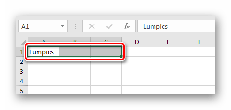
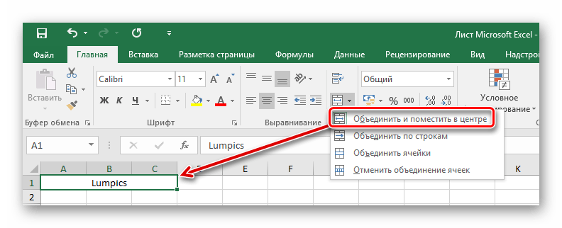
1. Последовательно выделите левой кнопкой мыши ячейки для слияния. Это могут быть строки, столбцы или совмещение вариантов. В рассмотренном методе используем объединение строки.



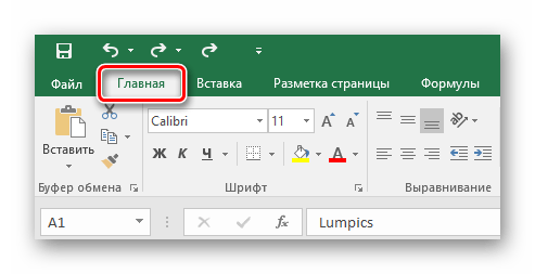
2. Перейдите во вкладку «Главная».



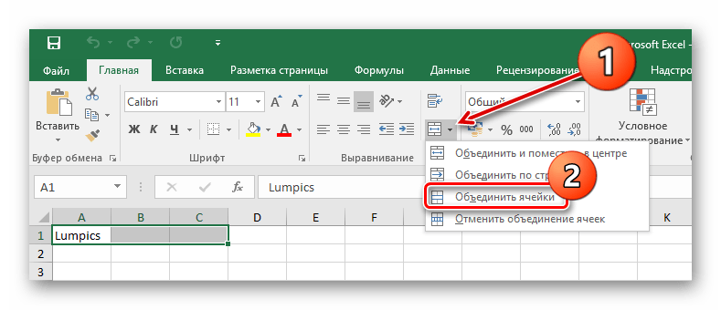
3. Найдите и нажмите на стрелку контекстного меню объединения, где есть несколько возможных вариантов, среди которых выберите самый простой из них — строку «Объединить ячейки».



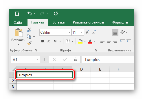
4. В этом случае ячейки объединятся, а все данные, которые будут вписываться в объединенную ячейку, останутся на прежнем месте.



5. Для форматирования текста после объединения по центру необходимо выбрать пункт «Объединение с выравниванием по центру». После проделанных действий содержимое можно выравнивать по-своему с помощью соответствующих инструментов.



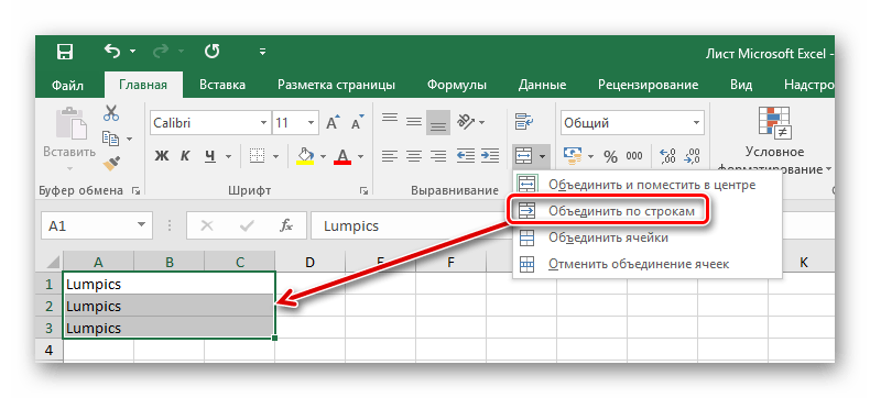
6. Чтобы не объединять большое количество строк по отдельности, воспользуйтесь функцией «Объединение по строкам».

Способ 2: Изменение свойств ячейки

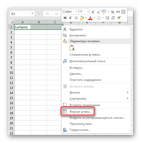
Существует возможность объединить ячейки через контекстное меню. Результат, получаемый из этого способа, не отличается от первого, но кому-то может быть удобнее в использовании.

1. Выделите курсором ячейки, которые следует объединить, кликните по ним правой кнопкой мыши, и в появившемся контекстном меню выберите пункт «Формат ячеек».



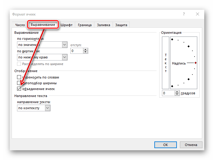
2. В открывшемся окне формата ячеек переходим во вкладку «Выравнивание». Отмечаем флажком пункт «Объединение ячеек». Тут же можно установить и другие параметры: направление и ориентация текста, выравнивание по горизонтали и вертикали, автоподбор ширины, перенос по словам. Когда все настройки выполнены, жмем на кнопку «OK».



3. Как видим, произошло объединение ячеек.

Способ 3: Объединение без потерь

Что делать, если в нескольких из объединяемых ячеек присутствуют данные, ведь при объединении все значения кроме левого верхнего будут утрачены? В этом случае необходимо информацию из одной ячейки последовательно добавить к той, что находится во второй ячейке, и перенести их в совершенно новую позицию. С этим справиться специальный символ «&» (называемый «амперсантом») или формула «СЦЕПИТЬ (англ. CONCAT)».

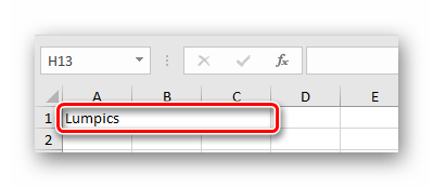
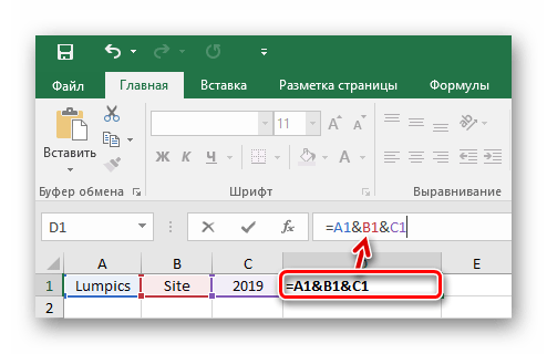
Начнём с более простого варианта. Всё, что нужно сделать — указать в новой ячейке путь к объединяемым ячейкам, а между ними вставить специальный символ. Давайте соединим сразу три ячейки в одну, создав таким образом текстовую строку.

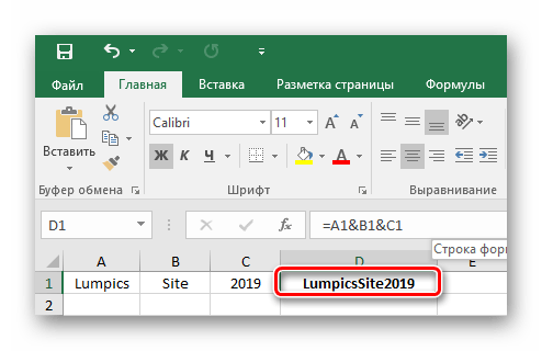
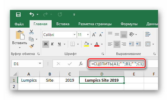
1. Выберите ячейку, в которой желаете увидеть результат объединения. В ней напишите знак равенства «=» и последовательно выберите конкретные позиции либо целый диапазон данных для слияния. Между каждой ячейкой или диапазоном следует внести знак амперсанта «&». В указанном примере мы объединяем клетки «A1», «B1», «C1» в одну — «D1». После ввода функции нажимаем «Enter».





2. Благодаря предыдущему действию в клетке с формулой слились все три позиции в одну.



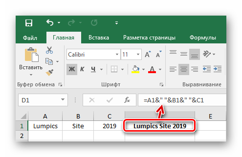
3. Чтобы текст в конце получился читабельным, между ячейками можно добавить пробелы. В любой формуле для добавления отступа между данными нужно ввести пробел в скобках. Поэтому, вставьте его между «A1», «B1» и «C1» таким образом: «=A1&» «&B1&» «&C1».



4. Формула предполагает примерно тот же принцип — указанные ячейки или диапазоны будут слиты в то место, где вы прописываете функцию «=СЦЕПИТЬ()». Рассматривая пример амперсанта, заменим его на упомянутую функцию: «=СЦЕПИТЬ(A1;» «;B1;» «;C1)». Обратите внимание, что для удобности сразу добавлены пробелы. В формуле пробел учитывается как отдельная позиция, то есть мы к ячейке «А1» добавляем пробел, затем ячейку «B1» и так далее.



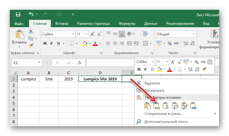
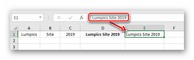
5. Если вам нужно избавиться от исходных данных, которые были использованы для объединения, оставив только результат, вы можете скопировать обработанную информацию как значение и удалить лишние колонки. Для этого скопируйте готовое значение в ячейке «D1» комбинацией клавиш «Ctrl + C», кликните правой кнопкой по свободной ячейке и выберите «Значения».



6. Как итог — чистый результат без формулы в ячейке. Теперь можно удалять предыдущую информацию удобным для вас способом.

Если обычное объединение ячеек в программе Microsoft Excel довольно простое, то с объединением ячеек без потерь придется повозиться. Тем не менее это тоже выполнимая задача для такого рода программы. Использование функций и специальных символов позволит сэкономить много времени на обработке большого объема информации.

Еще статьи по данной теме:

Помогла ли Вам статья?

Merged cells are one of the most popular options used by beginner spreadsheet users.

But they have a lot of drawbacks that make them a not so great option.

In this post, I’ll show you everything you need to know about merged cells including 8 ways to merge cells.

I’ll also tell you why you shouldn’t use them and a better alternative that will produce the same visual result.

What is a Merged Cell

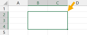
A merged cell in Excel combines two or more cells into one large cell. You can only merge contiguous cells that form a rectangular shape.

The above example shows a single merged cell resulting from merging 6 cells in the range B2:C4.

Why You Might Merge a Cell

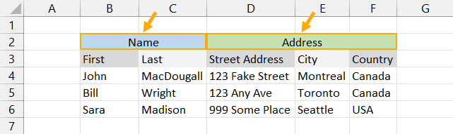
Merging cells is a common technique used when a title or label is needed for a group of cells, rows or columns.

When you merge cells, only the value or formula in the top left cell of the range is preserved and displayed in the resulting merged cell. Any other values or formulas are discarded.

The above example shows two merged cells in B2:C2 and D2:F2 which indicates the category of information in the columns below. For example the First and Last name columns are organized with a Name merged cell.

Why is the Merge Command Disabled?

On occasion, you might find the Merge & Center command in Excel is greyed out and not available to use.

There are two reasons why the Merge & Center command can become unavailable.

• You are trying to merge cells inside an Excel table.
• You are trying to merge cells in a protected sheet.

Cells inside an Excel table can not be merged and there is no solution to enable this.

If most of the other commands in the ribbon are greyed out too, then it’s likely the sheet is protected. In order to access the Merge option, you will need to unprotect the worksheet.

This can be done by going to the Review tab and clicking the Unprotect Sheet command.

If the sheet has been protected with a password, then you will need to enter it in order to unprotect the sheet.

Now you should be able to merge cells inside the sheet.

Merged Cells Only Retain the Top Left Values

Warning before you start merging cells!

If the cells contain data or formulas, then you will lose anything not in the upper left cell.

A warning dialog box will appear telling you Merging cells only keeps the upper-left value and discards other values.

The above example shows the result of merging cells B2:C4 which contains text data. Only the data from cell B2 remains in the resulting merged cells.

If no data is present in the selected cells, then no warning will appear when trying to merge cells.

8 Ways to Merge a Cell

Merging cells is an easy task to perform and there are a variety of places this command can be found.

Merge Cells with the Merge & Center Command in the Home Tab

The easiest way to merge cells is using the command found in the Home tab.

1. Select the cells you want to merge together.
2. Go to the Home tab.
3. Click on the Merge & Center command found in the Alignment section.

Merge Cells with the Alt Hotkey Shortcut

There is an easy way to access the Home tab Merge and Center command using the Alt key.

Press Alt H M C in sequence on your keyboard to use the Merge & Center command.

Merge Cells with the Format Cells Dialog Box

Merging cells is also available from the Format Cells dialog box. This is the menu which contains all formatting options including merging cells.

You can open the Format Cells dialog box a few different ways.

• Go to the Home tab and click on the small launch icon in the lower right corner of the Alignment section.
• Use the Ctrl + 1 keyboard shortcut.
• Right click on the selected cells and choose Format Cells.

Go to the Alignment tab in the Format Cells menu then check the Merge cells option and press the OK button.

Merge Cells with the Quick Access Toolbar

If you use the Merge & Center command a lot, then it might make sense to add it to the Quick Access Toolbar so it’s always readily available to use.

Go to the Home tab and right click on the Merge & Center command then choose Add to Quick Access Toolbar from the options.

This will add the command to your QAT which is always available to use.

A nice bonus that comes with the quick access command is it gets its own hotkey shortcut based on its position in the QAT. When you press the Alt key, Excel will show you what key to press next in order to access the command.

In the above example, the Merge and Center command is the third command in the QAT so the hotkey shortcut is Alt 3.

Merge Cells with Copy and Paste

If you have a merged cell in your sheet already then you can copy and paste it to create more merged cells. This will produce merged cells with the exact same dimensions.

Copy a merged cell using Ctrl + C then paste it into a new location using Ctrl + V. Just make sure the paste area doesn’t overlap an existing merged cell.

Merge Cells with VBA

Sub MergeCells()
    Range("B2:C4").Merge
End Sub

The basic command for merging cells in VBA is quite simple. The above code will merge cells B2:C4.

Merge Cells with Office Scripts

function main(workbook: ExcelScript.Workbook) {
	let selectedSheet = workbook.getActiveWorksheet();
	selectedSheet.getRange("B2:C4").merge(false);
	selectedSheet.getRange("B2:C4").getFormat().setHorizontalAlignment(ExcelScript.HorizontalAlignment.center);
}

The above office script will merge and center the range B2:C4.

Merge Cells inside a PivotTable

We can’t make this change for the selected cells because it will affect a PivotTable. Use the field list to change the report. If you are trying to insert or delete cells, move the PivotTable and try again.

If you try to use the Merge and Center command inside a Pivot Table, you will be greeted with the above error message.

You can’t use the Merge & Center command inside a PivotTable, but there is a way to merge cells in the PivotTable options menu.

In order to avail of this option, you will first need to make sure your Pivot Table is in the tabular display mode.

1. Select a cell inside your PivotTable.
2. Go to the Design tab.
3. Click on Report Layout.
4. Choose Show in Tabular Form.

Your pivot table will now be in the tabular form where each field you add to the Rows area will be in its own column with data in a displayed in a single row.

Now you can enable the option to show merge cells inside the pivot table.

1. Select a cell inside your PivotTable.
2. Go to the PivotTable Analyze tab.
3. Click on Options.

This will open up the PivotTable Options menu.

Enable the Merge and center cells with labels setting in the PivotTable Options menu.

1. Click on the Layout & Format tab.
2. Check the Merge and center cells with labels option.
3. Press the OK button.

Now as you expand and collapse fields in your pivot table, fields will merge when they have a common label.

10 Ways to Unmerge a Cell

Unmerging a cell is also quick and easy. Most methods involve the same steps as used to merge the cell, but there are a few extra methods worth knowing.

Unmerge Cells with the Home Tab Command

This is the same process as merging cells from the Home tab command.

1. Select the merged cells to unmerge.
2. Go to the Home tab.
3. Click on the Merge & Center command.

Unmerge Cells with the Format Cells Menu

You can unmerge cells from the Format Cells dialog box as well.

Press Ctrl + 1 to open the Format Cells menu then go to the Alignment tab then uncheck the Merge cells option and press the OK button.

Unmerge Cells with the Alt Hot Key Shortcut

You can use the same Alt hot key combination to unmerge a merged cell. Select the merged cell you want to unmerge then press Alt H M C in sequence to unmerge the cells.

Unmerge Cells with Copy and Paste

You can copy the format from a regular single cell to unmerge merged cells.

Find a single cell and use Ctrl + C to copy it, then select the merged cells and press Ctrl + V to paste the cell.

You can use the Paste Special options to avoid overwriting any data when pasting. Press Ctrl + Alt + V then select the Formats option.

Unmerge Cells with the Quick Access Toolbar

This is a great option if you have already added the Merge & Center command to the quick access toolbar previously.

All you need to do is select the merged cells and click on the command or use the Alt hot key shortcut.

Unmerge Cells with the Clear Formats Command

Merged cells are a type of format, so it’s possible to unmerge cells by clearing the format from the cell.

1. Select the merged cell to unmerge.
2. Go to the Home tab.
3. Click on the right part of the Clear button found in the Editing section.
4. Select Clear Formats from the options.

Unmerge Cells with VBA

Sub UnMergeCells()
    Range("B2:C4").UnMerge
End Sub

Above is the basic command for unmerging cells in VBA. This will unmerge cells B2:C4.

Unmerge Cells with Office Scripts

Most methods of merging a cell can be performed again to unmerge cells like a toggle switch to merge or unmerge.

However the code in office scripts doesn’t work like this and instead, you will need to remove formatting to unmerge.

function main(workbook: ExcelScript.Workbook) {
	let selectedSheet = workbook.getActiveWorksheet();
	selectedSheet.getRange("B2:C4").clear(ExcelScript.ClearApplyTo.formats);
}

The above code will clear the format in cells B2:C4 and unmerge any merged cells it contains.

Unmerge Cells with the Accessibility Pane

Merged cells create problems for screen readers which is an accessibility issue. Because of this, they are flagged in the Accessibility window pane.

If you know the location of the merged cells, you can select them and go to the Review tab then click on the lower part of the Check Accessibility button and choose Unmerge Cells.

If you don’t know where all the merged cells are, you can open up the accessibility pane and it will show you where there are and you will be able to unmerge them one by one.

Go to the Review tab and click on the top part of the Check Accessibility command to launch the accessibility window pane.

This will show a Merged Cells section which you can expand to see all merged cells in the workbook. Click on the address and Excel will take you to that location.

Click on the downward chevron icon to the right of the address and the Unmerge option can be selected.

Unmerge Cells inside a PivotTable

To unmerge cells inside a pivot table, you just need to disable the setting in the pivot table options menu.

Now you can enable the option to show merge cells inside the pivot table.

1. Select a cell inside your PivotTable.
2. Go to the PivotTable Analyze tab.
3. Click on Options.
4. Click on the Layout & Format tab.
5. Uncheck the Merge and center cells with labels option.
6. Press the OK button.

Merge Multiple Ranges in One Step

In Excel, you can select multiple non-continuous ranges in a sheet by holding the Ctrl key. A nice consequence of this is you can convert these multiple ranges into merged cells in one step.

Hold the Ctrl key while selecting multiple ranges with the mouse. When you’re finished selecting the ranges you can release the Ctrl key and then go to the Home tab and click on the Merge & Center command.

Each range will become its own merged cell.

Combine Data Before Merging Cells

Before you merge any cells which contain data, it’s advised to combine the data since only the data in the top left cell is preserved when merging cells.

There are a variety of ways to do this, but using the TEXTJOIN function is among the easiest and most flexible as it will allow you to separate each cell’s data using a delimiter if needed.

= TEXTJOIN ( ", ", TRUE, B2:C4 )

The above formula will join all the text in range B2:C4 going from left to right and then top to bottom. Text in each cell is separated with a comma and space.

Once you have the formula result, you can copy and paste it as a value so that the data is retained when you merge the cells.

How to Get Data from Merged Cells in Excel

A common misconception is that each cell of in the merged range contains the data entered inside.

In fact, only the top left cell will contain any data.

In the above example, the formula references the top left value in the merged range. The result returned is what is seen in the merged range.

In this example, the formula references a cell that is not the top left most cell in the merged range. The result is 0 because this cell is empty and contains no value.

In order to extract data from a merged range, you will always need to reference the top left most cell of the range. Fortunately, Excel automatically does this for you when you select the merged cell in a formula.

How to Find Merged Cells in a Workbook

If you create a bunch of merged cells, you might need to find them all later. Thankfully it’s not a painful process.

This can be done using the Find & Select command.

Go to the Home tab and click on the Find & Select button found in the Editing section, then choose the Find option. This will open the Find and Replace menu

You can also use the Ctrl + F keyboard shortcut.

You don’t need to enter any text to find, you can use this menu to find cells formatted as merged cells.

1. Click on the Format button to open the Find Format menu.
2. Go to the Alignment tab.
3. Check the Merge cells option.
4. Press the OK button in the Find Format menu.
5. Press the Find All or Find Next button in the Find and Replace menu.

Unmerge All Merged Cells

Fortunately, unmerging all merged cells in a sheet is very easy.

1. Select the entire sheet. You can do this two ways.
   • Click on the select all button where the column headings meet the row headings.
   • Press Ctrl + A on your keyboard.
2. Go to the Home tab.
3. Press the Merge & Center command.

This will unmerge all the merged cells and leave all the other cells unaffected.

Why You Shouldn’t Merge Cells

There are a lot of reasons why you shouldn’t merge cells.

• You can’t sort data with merged cells.
• You can’t filter data with merged cells.
• You can’t copy and paste values into merged cells.
• It will create accessibility problems for screen readers by changing the order in which text should be read.

This isn’t an exhaustive list, there are likely many more you will come across should you choose to merge cells.

Alternative to Merging a Cell

Good news!

There is a much better alternative than merging cells.

This alternative has none of the negative features that come with merging cells but will still allow you to achieve the same visual look of a merged cell.

It will allow you to display text centered across a range of cells without merging the cells.

Unfortunately, this technique will only work horizontally with one row of cells. There is no option to do something similar with a vertical range of cells.

Select the horizontal range of cells that you would like to center your text across. The first cell should contain the text which is to be centered while the remaining cells should be empty.

This example shows text in cell B2 and the range B2:C2 is selected as the range to center across.

Go to the Home tab and click on the small launch icon in the lower right corner of the Alignment section. This will open up the Format Cells dialog box with the Alignment tab active.

You can also press Ctrl + 1 to open the Format Cells dialog box and navigate to the Alignment tab.

Select Center Across Selection from the Horizontal dropdown options in the Text alignment section.

The text will now appear as though it occupies all cells but it will only exist in the first cell of the centering selection and each cell is still separate.

Pros

• The text appears centered across the selected range similar to a merged cell.
• No negative effects from merged cells.
• Can be used inside an Excel table.

Cons

• Can not center across a vertical range of cells.

Conclusions

There are lots of ways to merge cells in Excel. You can also easily unmerge cells too if you need to.

There are many things to consider when merging cells in Excel.

As you have seen, there are lots of pitfalls to merged cells that you should consider before implementing them in your workbooks.

Do you have a favorite merge method or warning about the dangers of merged cells that are not listed in the post? Let me know about it in the comments.