
This example shows two ways to compare text strings in Excel. One is case-sensitive and one is case-insensitive.
1. Use the EXACT function (case-sensitive).

Explanation: the string «Frog» in cell A1 and the string «frog» in cell B1 are not exactly equal to each other (first letter in uppercase and first letter in lowercase).
2. Use the formula =A1=B1 (case-insensitive).

Explanation: this formula ignores lowercase and uppercase differences. As a result, the first six formulas return TRUE.
3. Add the IF function to replace TRUE and FALSE with a word or message. The formula below uses the EXACT function (see step 1).

4. Do you want to compare two or more columns by highlighting the differences in each row? Visit our page about Row Differences.

Excel Text Compare (Table of Contents)
- Compare Text in Excel
- Methods to Compare Tex in Excel
- How to Compare Text in Excel?
How to Compare Text in Excel?
We compare data in MS Excel occasionally. There are several options as well available to do so in one column, but to determine the matches and differences in the different column, we have several techniques to compare it in Excel.
As Excel is versatile, there are several ways to compare the text, like full compare or a part of that text, where we can use other functions in Excel (LEFT, RIGHT, INDEX, MATCH, etc.).
Methods to Compare Text in Excel
The following method shows how to compare text in excel.
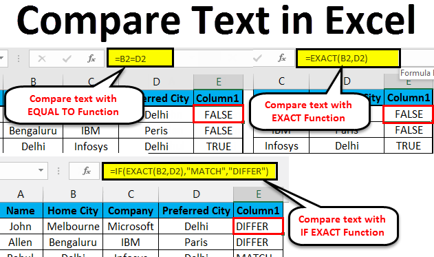
Method #1 – EXACT Function
If the two texts are identical, it is case sensitive; then it will return TRUE if not, then it will return FALSE.
Ex: There are two texts A1 is the ‘String’, and B1 is ‘string’ then result of the EXACT function will be FALSE
=EXACT (A1, B1) >> FALSE
Method #2 – Equal Sign (=)
It is case insensitive, so when we do not care about the case, we need to prefer this to compare the text. If the two texts are identical, then it will return TRUE if not, then it will return FALSE.
Ex: There are two texts A1 is the ‘String’, and B1 is ‘string’ then result of the function will be TRUE
=EXACT (A1, B1) >> TRUE
How to Compare Text in Excel?
To compare text in excel is very easy and simple to use. Let’s understand the working of compare text in excel with few examples.
You can download this Text Compare Excel Template here – Text Compare Excel Template
Compare Text in Excel – Example#1
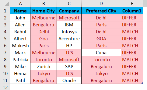
Comparing for the two City in the employee table in Excel without caring about the case of text, two texts are Home city and Preferred City.
Step 1: Go to Sheet 1 in the Excel sheet, which a user wants to compare.
Step 2: The user wants to check Home City and Preferred City, so apply the formula in the E column to compare in Excel
Step 3: Click on the E2 column and apply equal sign (=), Select B2 cell and put an equal sign, and select D2
(= B2=D2)
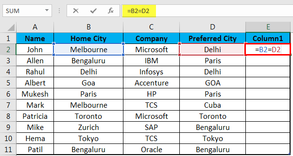
Step 4: Now click on the Enter button.
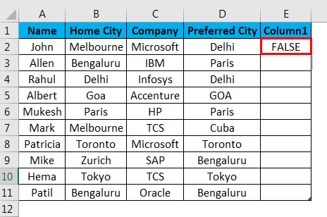
Step 5: Apply the above formula to all; we can drag down on clicking the Plus sign of the E2 cell.
Summary of Example #1: As we can see in the result of example 1, there is B2 in Melbourne, and D2 is Delhi which is not matching, so the result is FALSE. Similarly, in B4 and D4, we have Delhi, which matches, so the result is TRUE. If we see the 5th Row where B2 have Goa and D2 have GOA, their case is different in both the cells, but the equal function will not consider the case as it’s a case insensitive, so the result will be TRUE.
Compare Text in Excel – Example #2
How to Compare the column data in Excel, which the user wants to match with the case of text?
Step 1: Go to Sheet 2 in the excel sheet where a user wants to be compared the data; the user wants to check Home city and Preferred city, so apply the formula in the E column to compare.
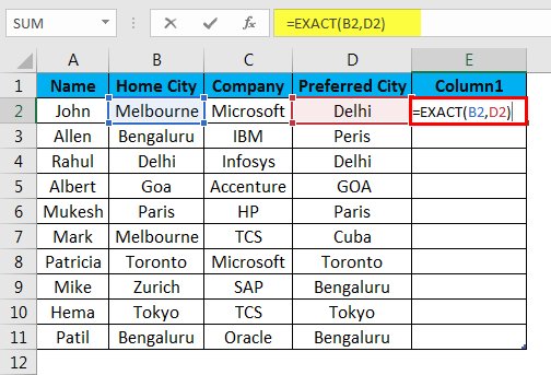
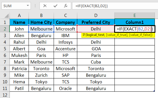
Step 2: Click on the E2 cell, apply the EXACT function, select the B2 cell, apply the EXACT function, and select D2.
(= EXACT (B2, D2)
Step 3: Now click on the Enter button, the result will be shown based on the input data.
Step 4: Apply the above formula to all; we can drag down on clicking the Plus sign of the E2 cell in the Excel sheet.
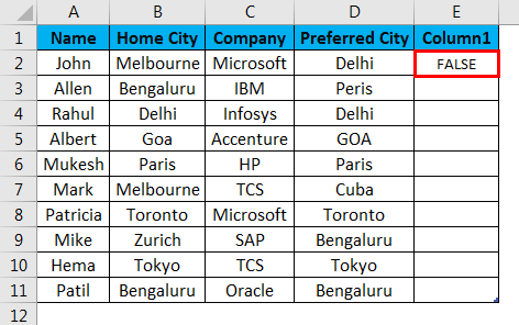
Summary of Example#2: As we can see in the result of the sheet 2 examples in Excel, there is B2 is Melbourne and D2 is Delhi which is not matching, so the result is FALSE. In B4 and D4, the same way has Delhi, which is matching, so the result is TRUE.
If we see the 5th Row where B2 have Goa and D2 have GOA, their case is different in both the cells, but the EXACT function will consider the case as its case sensitive, so the result will be FALSE. So, when we need to find the matching or difference in the text string with the case, then the EXACT function will do the task, but when we do not care about the case of the text string, then we can use the equal sign for comparing the data.
Compare Text in Excel – Example #3
How to compare the text in Excel, but the user wants some meaningful result rather than only TRUE/FALSE.
Step 1: Go to Sheet 3 in excel where a user wants to compare the data; the user wants to check Home City and Preferred City, so apply the formula in the E column to compare.
Step 2: Click on the E2 cell and apply the EXACT function with IF
Step 3: First write IF formula followed by EXACT, like =IF (EXACT (…))
Step 4: Now, Select B2 in Text 1 and D2 cells in Text 2 and close the bracket.
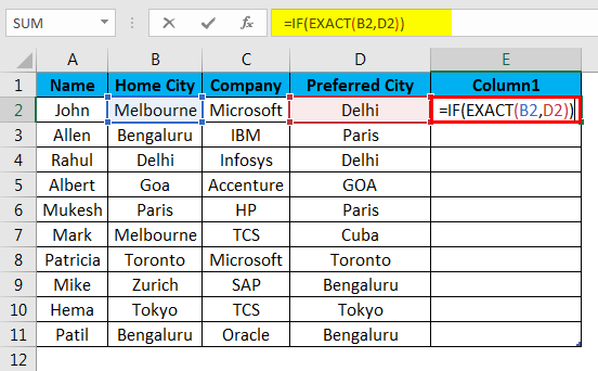
Step 5: Now, it will ask for value_if_true and value_if_false, put the value for the same.
Step 6: Now give Match if the value is true and Differ if the value is false and close the bracket.
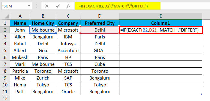
Step 7: Now click on the Enter button, the result will be shown based on the input data.
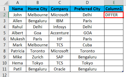
Step 8: Apply the above formula to all; we can drag down on clicking the Plus sign of the E2 cell.
Summary of Example#3: As we can see in the result of the sheet 3 examples, there is B2 is Melbourne and D2 is Delhi which is not matching, so the result is Differ. In B4 and D4, the same way has Delhi, which is matching, so the result is MATCH.
If we see the 5th Row where B2 has Goa and D2 has GOA, their case is different in both the cells, but the EXACT function will consider the case as its case sensitive, so the result will be Differ. Here we can see on being TRUE, we are getting output as Match, and when output is FALSE, we are getting Differ as to the output.
Things to Remember
- Using the Equal sign in Excel for comparison will treat GOA as goa because the equal sign is the case insensitive.
- As the EXACT function is case sensitive, we can go for an equal sign when we are not bothered about the case.
- We can use compare the result inside the IF function to show a meaningful message, or we can make it a conditional calculation.
- To see the duplicate data in the table, we need to select all the data and Press Ctrl + Q (Quick Analysis) >> then a pop-up will open up >> select Duplicate option >> it will highlight the duplicate.
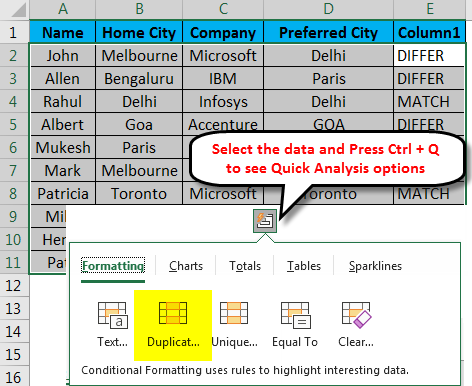
This is how we can compare the data in the table for duplicate and unique value.
- When we want to compare only a part of the text, then we can use the LEFT and RIGHT function.
Ex.=LEFT(A2,3) =RIGHT(B2,3)
Recommended Articles
This has been a guide to Text compare in excel. Here we discuss How to Compare Text in Excel, Methods used in Excel to Compare Text along with practical examples, and a downloadable excel template. You can also go through our other suggested articles –
- TEXT Function in Excel
- Excel Separate text
- Compare Two Lists in Excel
- VBA Text
Excel users often need to compare cells or columns to check if the same text is available in the cells/columns or not.
A very common example of this is when you have names in two columns and you want to check if the names are exactly the same or what names are missing in one column.
Comparing text in Excel is fairly easy and can be achieved with simple formulas.
In this tutorial, I will show you how to compare text in Excel using simple arithmetic operators or the EXACT function. I will also cover how you can compare text in two columns to find out the missing text entries.
Compare Text in Excel (Exact Cell against Cell Comparison)
Below I have a data set where I have names in column A as well as column B, and I want to compare the names in each row. I want to check whether the names in the same row are the same or not.

Let’s look at two simple ways to get this done.
Using the Equal to Operator
The equal operator can commit will pare the content in one cell with another cell, and give you a TRUE in case the cells have the exact same text in it, or FALSE in case the text is not the same.
Below is the formula that will compare the text in two cells in the same row:
=A2=B2
Enter this formula in cell C3 and then copy and paste it into all the cells.

The above formula returns a TRUE in case there is an exact match (meaning that the names are exactly the same), and it returns a FALSE in case the names do not match
In our example above, you can see that the formula returns FALSE in cells C6 and C11, indicating that the names in row #6 and row #11 are not the same.
If you want to only see the rows where the names are not the same, you can apply filters on the headers and then filter only those cells in column C where the value is FALSE
Note: For the formula to return a TRUE, the cell contents need to be exactly the same. In case there is an extra space in one of the cells, while it may look as if the cells have the same name, the formula would return a FALSE.
When you use the equal to operator, it does not consider the case of the text in the cell.
For example, if you have ‘James Baker’ in one cell and ‘james baker’ in another cell and you compare these two, the formula would return a TRUE.
In case you want the comparison to be case-sensitive, use the EXACT function method covered next.
Using the EXACT function
Another easy way to compare text in two cells in Excel is by using the EXACT function.
As the name suggests, it would return TRUE in case the content of the two cells being compared is exactly the same, and FALSE in case the contents are not the same.
Considering the same data set with names and column A and column B, below is the formula that will compare the names and give us the result
=EXACT(A2,B2)
Enter this formula in cell C3 and then copy and paste it into all the cells.

The EXACT function takes the cell reference of the cells that need to be compared as the arguments and returns a TRUE in case there is an exact match, and a FALSE if there is not.
In case you’re using newer versions of Excel that have dynamic arrays, you can also use the below formula in cell C2 (and you don’t need to copy and paste the formula in the remaining cells as the dynamic formula would spill over and fill the other cells automatically)
=EXACT(A2:A12,B2:B12)
Note that the EXACT function is case sensitive, so even if the names are exactly the same but in different cases (lower or upper, or proper), the formula would return a FALSE.
Compare Text and Find Missing Text Using VLOOKUP
Another real-life situation where you may need to compare text is when you have a list in two columns and you want to find out the items/names that are there in one column but missing in the other column.
Below I have a data set where I have some names in column A and in column B, and I want to check what names in column A are also they’re in column B, and which ones are missing

Below is the formula that would give us the text “Present” in case the name in column A is also there in column B and it would give us “Missing” in case the name in column A is not present in column B.
=IF(ISERROR(VLOOKUP(A2,$B$2:$B$9,1,0)),"Missing","Present")
Enter this formula in cell C3 and then copy and paste it into all the cells.

The above formula uses the VLOOKUP function to check for each name in column A against the list in column B.
If the VLOOKUP formula finds the name, it would return that name, and in case it doesn’t find the name, it would return the #N/A! error
I haven’t wrapped this VLOOKUP formula inside the ISERROR function so that if the names are present, it would return a FALSE, and if the names are missing then it would return a TRUE.
And then I wrapped this inside an IF function, which gives us the text ‘Present’ if the name in column A is also there in column B, as it returns the text ‘Missing’
You can also use a similar formula construct to check the other way around, whether the names in column B are present in column A or not (by adjusting the formula accordingly).
In this example, I have used the VLOOKUP function to compare the text in two columns, but this can also be done with other formulas such as INDEX/MATCH or XLOOKUP.
Compare Text and Check If Partial Text Matches
Another common situation that I have come across is when people want to compare the text in one cell with another cell, but they’re not looking for an exact comparison, and just need to check whether the text in one cell is present in the other cell or not.
Below I have a data set where I have some names in column A and in column B.

You would notice that the names in column B are only the first names, and the names in column A are full names.
Now I want to compare these two names and check whether the name in column B is there in column A or not.
As you can see, I’m not looking for an exact comparison but a partial text match.
And below is the formula that will do this for me:
=ISNUMBER(FIND(B2,A2))
Enter this formula in cell C3 and then copy and paste it into all the cells.

The above formula uses the FIND function to check whether the text value in column B is present in the cell in column A or not.
If the FIND function finds the text in column A it would return the starting position of that text (i.e., it would return a numeric value), and if it cannot find the text, it would return the VALUE error.
I have wrapped the FIND function inside the ISNUMBER function, which would return a TRUE in case the FIND function found the text in column A and returned a value, otherwise, it would return a FALSE.
In this tutorial, I covered some simple formulas that you can use to quickly compare text in Excel.
If you’re looking to compare one cell with another, you can use the equal-to operator or the EXACT function.
And if you’re trying to compare two columns, you can use the VLOOKUP function. And finally, I’ve also covered a method to show you how to compare partial text using the find function.
Other Excel tutorials you may also like:
- How to Compare Two Excel Sheets (for differences)
- How to Compare Dates in Excel (Greater/Less Than, Mismatches)
- How to Compare Two Columns in Excel (for matches & differences)
- Separate Text and Numbers in Excel (4 Easy Ways)
- How To Remove Text Before Or After a Specific Character In Excel
Compare Text
- Use the EXACT function (case-sensitive).
- Use the formula =A1=B1 (case-insensitive).
- Add the IF function to replace TRUE and FALSE with a word or message.
- Do you want to compare two or more columns by highlighting the differences in each row?
Contents
- 1 How do I identify similar text in Excel?
- 2 How do I compare two text columns in Excel for differences?
- 3 How do I compare multiple text in Excel?
- 4 How do I compare partial text in Excel?
- 5 What is an Xlookup in Excel?
- 6 How do you compare data in two Excel sheets for matches?
- 7 How do I compare two columns in Excel to match?
- 8 How do I compare two texts?
- 9 How do I find similar text in two columns in Excel?
- 10 How do I count partial text in Excel?
- 11 How do you check if a cell contains a specific text in Excel?
- 12 How do I match text from two sheets in Excel?
- 13 Is Xlookup better than VLOOKUP?
- 14 Is Xlookup faster than VLOOKUP?
- 15 How do I enable Xlookup?
- 16 How do you compare two Excel sheets and find differences?
- 17 How do I open a compare spreadsheet?
- 18 How do you compare two Excel files using beyond compare?
- 19 How does a Vlookup work?
- 20 How do I count matching values in Excel?
How do I identify similar text in Excel?
How to find similar values in multiple lists using the Exact function in Excel
- Select cell E2. Then select the Formulas tab, and select Text.
- Select Exact.
- Ensure the cursor is in the first text box (Text1) and select cell A2.
- Then click in the second text box (Text2) and select cell C2.
- Select OK.
How do I compare two text columns in Excel for differences?
Compare Two Columns and Highlight Matches
- Select the entire data set.
- Click the Home tab.
- In the Styles group, click on the ‘Conditional Formatting’ option.
- Hover the cursor on the Highlight Cell Rules option.
- Click on Duplicate Values.
- In the Duplicate Values dialog box, make sure ‘Duplicate’ is selected.
How do I compare multiple text in Excel?
How to compare if multiple cells are equal in Excel?
- Compare if multiple cells are equal with formulas.
- In a blank cell besides your data, please enter this formula: =AND(EXACT(A1:D1,A1)), (A1:D1 indicates the cells that you want to compare, and A1 is the first value in your data range)see screenshot:
How do I compare partial text in Excel?
If you just want to find which name is partial match the given name, you also can use this formula =INDEX($E$2:$E$14,MATCH($K$1&”*”,E2:E14,0)). (E2:E14 is the column list you want to lookup from, k1 is the given name, you can change as you need.)
What is an Xlookup in Excel?
Use the XLOOKUP function to find things in a table or range by row.With XLOOKUP, you can look in one column for a search term, and return a result from the same row in another column, regardless of which side the return column is on.
How do you compare data in two Excel sheets for matches?
Select both columns of data that you want to compare. On the Home tab, in the Styles grouping, under the Conditional Formatting drop down choose Highlight Cells Rules, then Duplicate Values. On the Duplicate Values dialog box select the colors you want and click OK. Notice Unique is also a choice.
How do I compare two columns in Excel to match?
Excel allows a user to compare two columns by using the SUMPRODUCT function.
Using the SUMPRODUCT to Count Matches Between Two Columns
- Select cell F2 and click on it.
- Insert the formula: =SUMPRODUCT(–(B3:B12 = C3:C12))
- Press enter.
How do I compare two texts?
How to Compare Document Text Using Windows 10
- In the search box on the toolbar type Word.
- Select Word from the search options.
- On the MS Word toolbar click Review.
- In the Review menu, click Compare.
- From the two options available, select Compare…
How do I find similar text in two columns in Excel?
Example 1. Compare two columns for matches or differences in the same row
- To compare two columns in Excel row-by-row, write a usual IF formula that compares the first two cells.
- The result may look similar to this:
- =IF(EXACT(A2, B2), “Match”, “”)
- =IF(AND(A2=B2, A2=C2), “Full match”, “”)
How do I count partial text in Excel?
Select a blank cell you will place the counting result at, type the formula =COUNTIF(A1:A16,”*Anne*”) (A1:A16 is the range you will count cells, and Anne is the certain partial string) into it, and press the Enter key. And then it counts out the total number of cells containing the partial string.
How do you check if a cell contains a specific text in Excel?
To check if a cell contains specific text, use ISNUMBER and SEARCH in Excel. There’s no CONTAINS function in Excel. 1. To find the position of a substring in a text string, use the SEARCH function.
How do I match text from two sheets in Excel?
How to use the Compare Sheets wizard
- Step 1: Select your worksheets and ranges. In the list of open books, choose the sheets you are going to compare.
- Step 2: Specify the comparing mode.
- Step 3: Select the key columns (if there are any)
- Step 4: Choose your comparison options.
Is Xlookup better than VLOOKUP?
The XLOOKUP defaults to an exact match where the VLOOKUP defaults to an approximate match. As the exact match is used most often, this setting would make the XLOOKUP more effective. On top of this, the XLOOKUP offers an additional option of an approximate match returning the next larger value.
Is Xlookup faster than VLOOKUP?
Compared to a normal VLOOKUP, the binary XLOOKUP is significantly faster. But a VLOOKUP with a approximate match is still a little bit faster. The binary XLOOKUP is slightly slower than an approximate VLOOKUP (~16% slower).
How do I enable Xlookup?
- Position the cell cursor in cell E4 of the worksheet.
- Click the Lookup & Reference option on the Formulas tab followed by XLOOKUP near the bottom of the drop-down menu to open its Function Arguments dialog box.
- Click cell D4 in the worksheet to enter its cell reference into the Lookup_value argument text box.
How do you compare two Excel sheets and find differences?
Compare Two Sheets and Highlight Differences (Using Conditional Formatting)
- Select the data in the sheet where you want to highlight the changes.
- Click the Home tab.
- In the Styles group, click on ‘Conditional Formatting’
- In the options that show up, click on ‘New Rule’
How do I open a compare spreadsheet?
Compare two versions of a workbook by using Spreadsheet Compare
- Open Spreadsheet Compare.
- In the lower-left pane, choose the options you want included in the workbook comparison, such as formulas, cell formatting, or macros.
- On the Home tab, choose Compare Files.
How do you compare two Excel files using beyond compare?
Beyond Compare’s Table Compare session will open and compare the current sheet in the Excel file.
- Open your . XLS or . XLSX file in Excel.
- Switch the visible sheet to the sheet you wish to compare.
- Save the Excel file.
- Open and compare the file in Beyond Compare.
How does a Vlookup work?
The VLOOKUP function performs a vertical lookup by searching for a value in the first column of a table and returning the value in the same row in the index_number position.As a worksheet function, the VLOOKUP function can be entered as part of a formula in a cell of a worksheet.
How do I count matching values in Excel?
Count cells equal to
- Generic formula. =COUNTIF(range,value)
- To count the number of cells equal to a specific value, you can use the COUNTIF function.
- The COUNTIF function is fully automatic — it counts the number of cells in a range that match the supplied criteria.
- Excel COUNTIF Function.
- Excel’s RACON functions.
By default, Excel is not case-sensitive. For example, with «APPLE» in A1, and «apple» in A2, the following formula will return TRUE:
=A1=A2 // returns TRUE
To compare text strings in a case-sensitive way, you can use the EXACT function. The Excel EXACT function compares two text strings, taking into account upper and lower case characters, and returns TRUE if they are the same, and FALSE if not.
If we use EXACT to compare A1 and A2 as above, the result is FALSE:
=EXACT(A1,A2) // returns FALSE
EXACT with IF
You can use this result inside the IF function to display a message or make a conditional calculation. For example, to display the message «Yes» for a match and «No» if not, you can use a formula like this:
=IF(EXACT(A2,A2),"Yes","No")