How to Compare Two Lists in Excel? (Top 6 Methods)
Below are the six different methods used to compare two lists of a column in Excel for matches and differences.
- Method 1: Compare Two Lists Using Equal Sign Operator
- Method 2: Match Data by Using the Row Difference Technique
- Method 3: Match Row Difference by Using the IF Condition
- Method 4: Match Data Even If There is a Row Difference
- Method 5: Highlight All the Matching Data using Conditional Formatting
- Method 6: Partial Matching Technique
Table of contents
- How to Compare Two Lists in Excel? (Top 6 Methods)
- #1 Compare Two Lists Using Equal Sign Operator
- #2 Match Data by Using Row Difference Technique
- #3 Match Row Difference by Using IF Condition
- #4 Match Data Even If There is a Row Difference
- #5 Highlight All the Matching Data
- #6 Partial Matching Technique
- Things to Remember
- Recommended Articles
Now, let us discuss each of the methods in detail with an example: –
You can download this Compare Two Lists Excel Template here – Compare Two Lists Excel Template
#1 Compare Two Lists Using Equal Sign Operator
We must follow the below steps to compare the two lists.
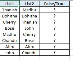
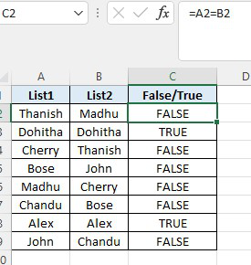
- Immediately after the two columns, we must insert a new column called “Status” in the next column.

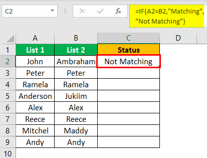
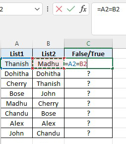
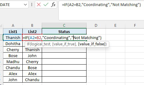
- Now, we must put the formula in cell C2 as =A2=B2.

- This formula tests whether the cell A2 value is equal to cell B2. If both cell values are matched, we will get TRUE or FALSE results.

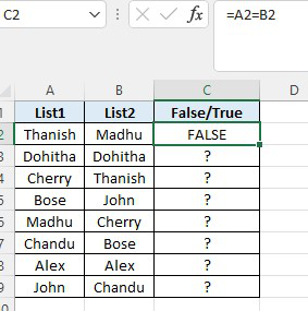
- We will drag the formula to cell C9 to determine the other values.


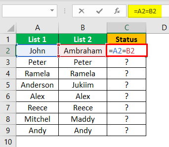

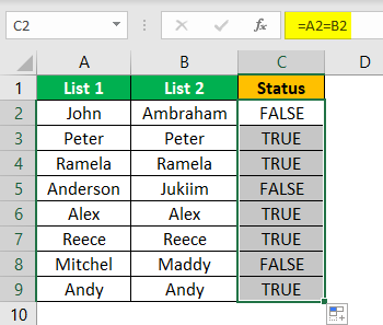
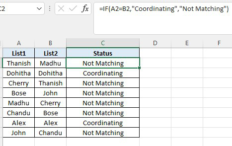
Wherever we have the same values in common rows, we get the result as “TRUE” or “FALSE.”
#2 Match Data by Using Row Difference Technique
You might not have used the “Row Difference” technique at your workplace. But today, we will show you how to use this technique to match data row by row.
- Step 1: To highlight non-matching cells row by row, we must select the entire data first.

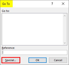
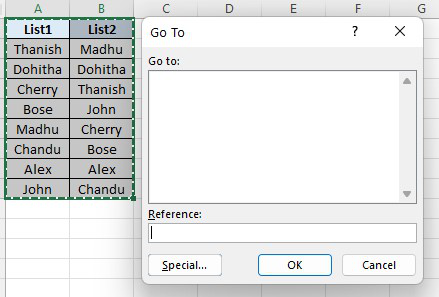
- Step 2: Now, we must press the excel shortcut keyAn Excel shortcut is a technique of performing a manual task in a quicker way.read more “F5” to open the “Go to Special” tool.
![]()
- Step 3: Press the “F5” key to open this window. In the “Go To” window, press the “Special” tab.

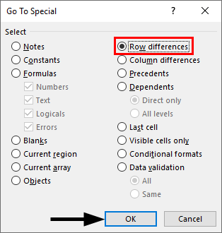
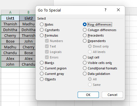
- Step 4: In the next window, we must go to the “Go To Special” and choose the “Row differences” option. Then, click on “OK.”

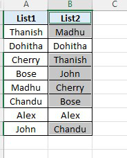
We will get the following result.

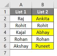
As shown in the above window, it has selected the cells wherever there is a row difference. Therefore, we must fill in some colors to highlight the row difference values.

#3 Match Row Difference by Using IF Condition
How can we leave out the IF condition when we want to match data row by row? In the first example, we have either “TRUE” or “FALSE.” But what if we need a different result instead of the default results of either “TRUE or FALSE.” Assume we need a result as “Matching” if there is no row difference, and the result should be “Not Matching” if there is a row difference.
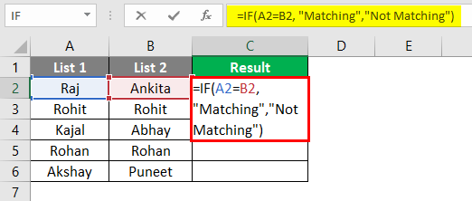
- Step 1: First, we must open the IF condition in cell C2.

- Step 2: Then, apply the logical testA logical test in Excel results in an analytical output, either true or false. The equals to operator, “=,” is the most commonly used logical test.read more as A2=B2.
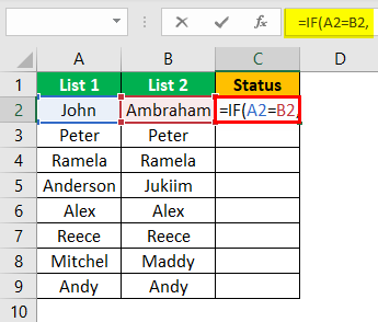
- Step 3: We must enter the result criteria if the logical test is “TRUE.” In this scenario, the result criteria are “Matching,” If the row does not match, we need the result as “Not Matching.”

- Step 4: Next, we need to apply the formula to get the result.
- Step 5: We must drag the formula to cell C9 to determine the other values.

#4 Match Data Even If There is a Row Difference
The matching data on the row differences method may not always work; the value may be in other cells too. So we need to use different technologies in these scenarios.
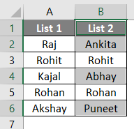
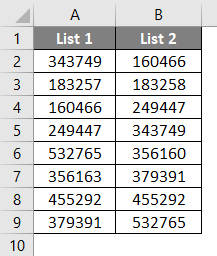
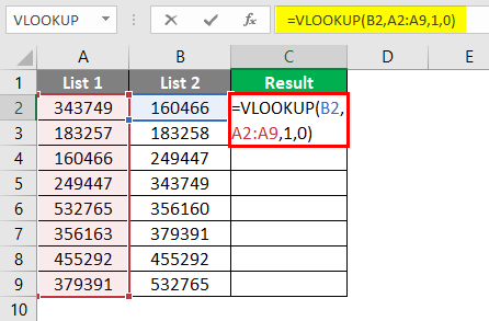
Now, look at the below data.

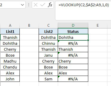
In the above image, we have two lists of numbers. We need to compare list 2 wish list 1. So let us use our favorite function VLOOKUPThe VLOOKUP excel function searches for a particular value and returns a corresponding match based on a unique identifier. A unique identifier is uniquely associated with all the records of the database. For instance, employee ID, student roll number, customer contact number, seller email address, etc., are unique identifiers.
read more.

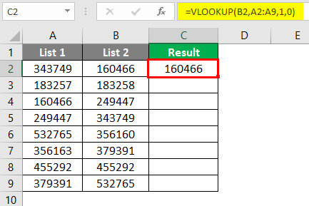
So, if the data matches, we get the number; otherwise, we get the error value as #N/A.
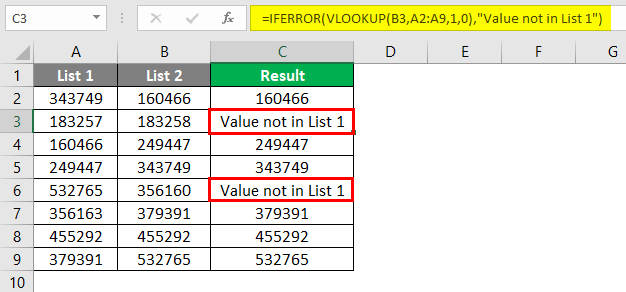
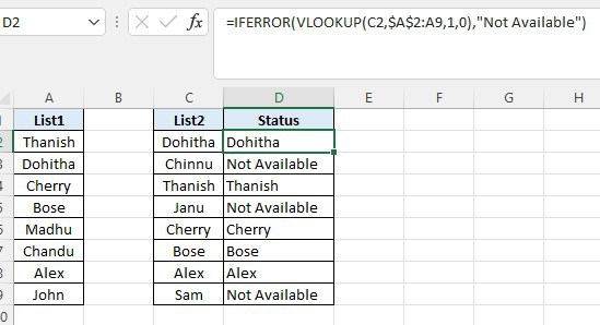
Showing error values does not look good. So instead of showing the error, let us replace them with the word “Not Available.” For this, use the IFERROR function in ExcelThe IFERROR function in Excel checks a formula (or a cell) for errors and returns a specified value in place of the error.read more.

#5 Highlight All the Matching Data
If you are not a fan of Excel formulasThe term «basic excel formula» refers to the general functions used in Microsoft Excel to do simple calculations such as addition, average, and comparison. SUM, COUNT, COUNTA, COUNTBLANK, AVERAGE, MIN Excel, MAX Excel, LEN Excel, TRIM Excel, IF Excel are the top ten excel formulas and functions.read more, do not worry. We can still match data without the formula. For example, using simple conditional formatting in ExcelConditional formatting is a technique in Excel that allows us to format cells in a worksheet based on certain conditions. It can be found in the styles section of the Home tab.read more, we can highlight all the matching data of two lists.
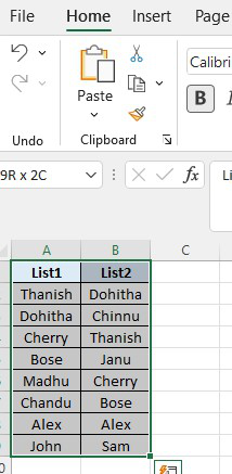
- Step 1: We must first select the data.

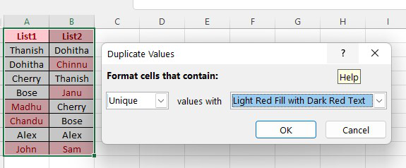
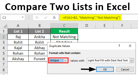
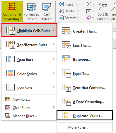
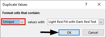
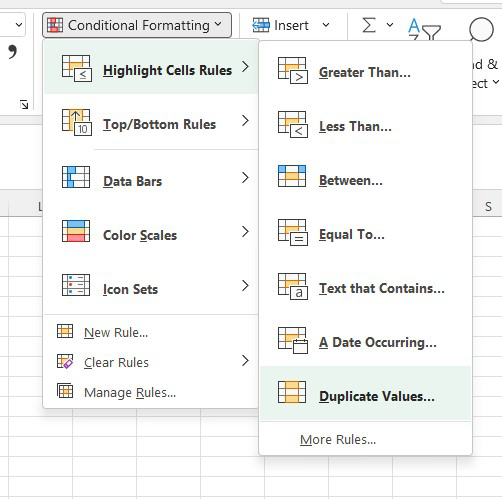
- Step 2: Now, we must go to “Conditional Formatting” and choose “Highlight Cell Rules” >> “Duplicate Values.”

- Step 3: As a result, we can see the “Duplicate Cell Values” formatting window.

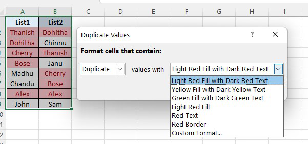
- Step 4: We can choose the different formatting colors from the drop-down list in ExcelA drop-down list in excel is a pre-defined list of inputs that allows users to select an option.read more. Select the first formatting color and press the “OK” button.

- Step 5: This will highlight all the matching data from the two lists.

- Step 6: Just in case, instead of highlighting all the matching data, if we want to highlight not matching data, then we can go to the “Duplicate Values” window and choose the option “Unique.”

As a result, it will highlight all the non-matching values, as shown below.

#6 Partial Matching Technique
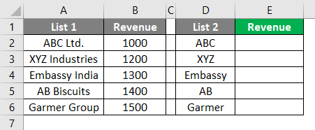
We have seen the issue of not having full or the same data in two lists. For example, if the List 1 data has “ABC Pvt Ltd.“ In List 2, we have “ABC” only. In these cases, all our default formulas and tools are not recognized. Therefore, we need to employ the special character asterisk (*) to match partial values in these cases.

In List 1, we have the company name and revenue details. In List 2, we have company names but not exact values as in List 1. It is a tricky situation that we all have faced at our workplace.
In such cases, still, we can match data by using a special character asterisk (*).

We get the following result.

We will drag the formula to cell E9 to determine the other values.

The wildcard character asterisk (*) was used to represent any number of characters so that it will match the full character for the word “ABC” as “ABC Pvt Ltd.”
Things to Remember
- The use of the above techniques for comparing two lists in Excel upon the data structure.
- If the data is not organized, row-by-row matching is not the best suited.
- VLOOKUP is the often-used formula to match values.
Recommended Articles
This article is a guide to Compare Two Lists in Excel. We discuss the top 6 methods to compare two columns list in Excel for the match, along with examples and a downloadable Excel template. You may learn more about Excel from the following articles: –
- Compare Two Excel Columns Using Vlookup
- Partial Match with Vlookup
- Compare Two Excel Columns
- Shade Alternate Rows in Excel
Hay Paula, can you compare lists in Excel?
or
What is the best way to compare two sets of data in Excel?
Very often there is a requirement in Excel to compare two lists, or two data sets to find missing or matching items. As this is Excel, there are always more than one way to do things, including comparing data. From formulas and Conditional Formatting to Power Query. In this article we are going to look at a number ways to compare two lists in Excel and we will also look at comparing entire rows of a data set.
Maybe your preferred way is not included below. If not why don’t you drop a comment below and share with us how you like to compare two lists or datasets in Excel. I look forward to reading your comments.
We wish to compare List 1 with List 2.

Contents
Quick Conditional Formatting to compare two columns of data
Clearing the Conditional Formatting
Match data in Excel using the MATCH function
Compare 2 lists in Excel 365 with MATCH or XMATCH as a Dynamic Array function
MATCH and Dynamic arrays to compare 2 lists
XMATCH Excel 365 to compare two lists
Tables – Comparing lists in Excel where the ranges sizes might change
Highlight differences in Lists using Custom Conditional Formatting
Copy formula to Custom Conditional Formatting
Other Formulas used to compare two lists in Excel
VLOOKUP to compare two lists in Excel
XLOOKUP to compare two lists in Excel
COUNTIF to compare two lists in Excel
How to compare 2 data sets in Excel
Comparing lists or datasets using Power Query

Quick Conditional Formatting to compare two columns of data
Conditional formatting will allow you to highlight a cells or range based on predefined criteria. The quickest and simplest way to visually compare these two columns quickly is to use the predefined highlight duplicate value rule.
Start by selecting the two columns of data.
From the Home tab, select the Conditional Formatting drop down. Then select Highlight Cells Rules. Next select Duplicate values.

A Duplicate Values settings box will open where you can define the formatting and select between Duplicate or Unique values.

By Selecting Duplicate, all reoccurring entries will be set to the selected formatting. Now you can quickly see the items in List 1 that are in List 2 as these are the formatted items. You can also quickly see the items in list 2 that are not in list 1 as these do not have formatting applied.

However, you can also format the Unique items. This can be achieved by selecting Unique from the Duplicate Values setup box.

In this case, we have applied two different conditional formats. The red indicating the duplicates and the green indicating the unique items.
Note, I did not just take the cells with data, I grabbed all of columns A to C. Column B has no data, so it cannot affect the results. However, these cells do contain the conditional formatting applied so it would be better practice to only select the cells you need.
Clearing the Conditional Formatting
To clear all conditional formatting, first select the cell, or range. Then select the conditional formatting drop down on the Home ribbon. Next select Clear Rules. Finally Select Clear Rules from Selected Cells.

If you have more than one conditional formatting applied at once and you only want to remove one of these, select Manage Rules from the conditional formatting drop down. Select the rule you want to delete and then select Delete Rule.

By pressing OK, the rule will removed from the Rules Manager and the cells will no longer contain the formatting.

So that is the most basic way you can compare two lists in Excel. Its quick, its simple and it is effective. You can also apply conditional formatting based on formulas, which we will look at later in this article.
Match data in Excel using the MATCH function
There are many lookup formulas that you can use to compare two ranges or lists in Excel. The first we will look at is the MATCH function.
The MATCH function returns the relative position in a list. A number based on its position, if found, in the lookup array.
The syntax for MATCH is
=MATCH (lookup value, Lookup array, Match type)
Where lookup value is the value you want to find a match for. Lookup array is the list in which you are looking for a match. And Match type allows you to select between an exact or approximate match.
We want to write a match formula to see if the items in List 2 are in List 1.
In cell E3 we can enter the formula
=MATCH(C2, $A$2:$A$21,0)

By filling this formula down, for the values where Excel finds a match, the position of that match will be returned. Where there is no match the return value will be an #N/A.

Very often, the relative position or the #N/A is of no value to us and we need to convert these values into true or false. To do this we can easily expand on our Match formula using a logical function. As Match returns a number, we can use the ISNUMBER function
=ISNUMBER(MATCH(C2, $A$2:$A$21,0))

Compare 2 lists in Excel 365 with MATCH or XMATCH as a Dynamic Array function
If you are using Excel 365 you have further alternatives when using MATCH to compare lists or data. As Excel 365 thinks in arrays, we can now pass an array as the lookup value of MATCH and our results will spill for us. This removes the need to copy the formula down and with only 1 formula, your spreadsheet will be less prone to errors and more compact.
MATCH and Dynamic arrays to compare 2 lists
If you are not yet familiar with Dynamic Arrays, I would suggest you have a read of this article: Excel Dynamic Arrays – A new way to model your Excel Spreadsheets: to get a better understand on how they work and spill ranges.
The only change to the match formula is instead of selecting cell C2 as our lookup value we will select the range C2:12
=ISNUMBER(MATCH (C2:C12,$A$2:$A$21,0))

As you can see, the one formula spills the results down column E.
XMATCH Excel 365 to compare two lists
Excel 365 also introduces the new function XMATCH. Just like the MATCH function XMATCH returns a relative position in a list. Now you are familiar XLOOKUP, which replaces the old VLOOKUP function, you know XLOOKUP comes with additional power. This come in the form of new conditions in the formula syntax such as search mode and match types. Well, XMATCH also as this extra power over its predecessor MATCH.
The syntax for XMATCH is
XMATCH (Lookup Value, Lookup Array, [Match Mode],[Search Mode])
Where
Lookup Value is the value you are looking to find the relative position
Lookup Array is the row or column that contains the Lookup Value
Match mode is optional. Unlike the old MATCH function, the default is an exact match. You can also select between
- Exact match or next smallest
- Exact match or next largest
- Wildcard match
Search mode is also optional. The default (and only option in the old MATCH function) is to look from the top down. You can also select last to first and binary searches. If you are working with binary searches. The wildcard match option does not work.
With XMATCH we can use either Dynamic arrays or cell references to create the formula, just like we have looked at with MATCH. For this example, we will use Dynamic Arrays. The formula is very similar to what we used with MATCH; except we do not have to select 0 for an exact match as in XMATCH this is the default setting. Let us mix things up a little this time a look at finding items in list 2 not in list one.
In this case we can use the formula
=NOT(ISNUMBER(XMATCH(C2:C12,A2:A21)))
Where not will turn trues into false and false into trues.

Tables – Comparing lists in Excel where the ranges sizes might change
In each of the formulas we have looked at so far, we have selected a range of cells in our Match functions that is not dynamic. That means if we add new data to one of the lists, we have a manual step to update our formula to include the new data.
To convert the lists to tables, select one of the lists and press CTRL. This is the keyboard shortcut to convert to a table. If you selected the header in the range of cells, ensure you tick the box to confirm your table has headers.

Tables by their nature use structured naming. Therefore, when you are writing a formula and you select a column from a table, it will not show cell references, but the column name.
Looking at our previous formula using XMATCH to find items in list 2 not in list 1, we can re-write this function now using our table references
=NOT (ISNUMBER(XMATCH(list2[List 2],list1[List 1])))

Now, as we have used tables, if we add a new row to either of the tables, our spill range will also increase to include the new data.

Highlight differences in Lists using Custom Conditional Formatting
Earlier in this article we looked at a very quick way of comparing these two lists using a predefined rule for duplicates. We can however also use Custom Conditional Formatting. If you are not familiar with Custom Conditional Formatting, I would suggest you check out this article: Excel Dynamic Conditional Formatting Tricks:
We need to look at two different approaches here to highlighting differences. When we are not using tables and we have created a true/false formula to identify the differences, we can take a copy of the formula and add this to our Custom formatting. However, with Tables we need to force the use of cell references.
Copy formula to Custom Conditional Formatting
Start by taking a copy of the formula. As we have tested the formula in the spreadsheet, we can see that it works before we use it in conditional formatting. This is best practice as very often with relative and absolute cell references it can be difficult to get the formula correct.

Select the cells that you want to apply the custom formatting to. Then from the Home ribbon select the conditional formatting drop down and select New Rule

The New Formatting Rule set up box will open and select Use Formula to determine which cells to format. Then paste in the formula and set the formatting type

This will result in all cells that are in both lists being formatted to your chosen format.

Keep in mind that we selected a range of cells to apply this conditional formatting and it is not dynamic. Should we use tables, this would update without the need to change anything!
Other Formulas used to compare two lists in Excel
There are many formulas you can use to compare two lists in Excel. We have already looked at MATCH and XMATCH, but now we are going to look at a few more. Any of the lookup functions will really work along with some others!
VLOOKUP to compare two lists in Excel
If you are not familiar with VLOOKUP, you can read about it here. Simply put VLOOKUP will return a corresponding value from a cell, if there is no corresponding value an #N/A error will be returned. In our example we are working with text. So, we can carry out a VLOOKUP and test to see if it returns text. If we were using numbers then we could replace ISTEXT with ISNUMBER.
We could use the function =ISTEXT(VLOOKUP(C2, $A$2:$A$21,1,FALSE))

Or if we were using Dynamic arrays in Excel 365, we could use the function
=ISTEXT(VLOOKUP (C2:C12,$A$2:$A$21,1,FALSE))

XLOOKUP to compare two lists in Excel
XLOOKUP was introduced in Excel 365 and you can find out more about it here. Very much like VLOOKUP, XLOOKUP will return a corresponding value from a cell, and you can define a result if the value is not found. Using Dynamic arrays, the function would be
=ISTEXT(XLOOKUP (C2:C12,A2:A21,A2:A21))

COUNTIF to compare two lists in Excel
The COUNTIF function will count the number of times a value, or text is contained within a range. If the value is not found, 0 is returned. We can combine this with an IF statement to return our true and false values.
=IF(COUNTIF (A2:A21,C2:C12)<>0,”True”, “False”)

How to compare 2 data sets in Excel
Comparing two lists is easy enough and we have looked now at several ways to do this. But comparing two data sets can be a little more difficult.
Let us look at an example. We have two tables of data, each containing the same column headers. Looking at the image, we can see matching these two tables would require looking at more than one column.

When you need to look at more than one column, the solution would be to create a composite column combining the data into one column. This will create a unique column for each row which we can then use as the matching column
In this example we could combine the Name and DoB to give each table a unique identifier
There are many ways to join contents of a cell, in this case we will do a simple concatenate. As we are using tables, the formula will shoe the table naming format.
=[@Name] &”-“&[@DoB]

Repeat the steps on the second table.
Now we can use any of the examples above to match these two new columns of data. Where they match, we know they match the entire row.

Comparing lists or datasets using Power Query
You can also compare lists and datasets using Excels Power Query. By connecting to the tables and then merging the tables, using different join types we can compare both lists.
In this video you will learn how to compare or reconcile two different data sets using Excels Power query
There is a data set to go along with this video and practice along which you can grab from this article.
However very often you will have datasets where there is no matching column and we need to create a column to carry out a reconciliation between two different lists or two different data sources. In this video you will learn how to create a matching column using power query so you can then compare the data.
A Ridiculously easy and fun way to compare 2 lists
- Select cells in both lists (select first list, then hold CTRL key and then select the second)
- Go to Conditional Formatting > Highlight Cells Rules > Duplicate Values.
- Press ok.
- There is nothing do here. Go out and play!
Contents
- 1 How do you compare two lists in Excel to see what is missing?
- 2 How do I compare two sets of data in Excel?
- 3 What is the best way to compare two lists in Excel?
- 4 How do you compare data sets?
- 5 What is Vlookup in Excel?
- 6 How do you compare two lists in Excel and pull matching data?
- 7 How do I match data from two Excel spreadsheets?
- 8 How do I compare two columns in Excel and return the third column?
- 9 How do I compare list names in Excel?
- 10 How do I compare 4 lists in Excel?
- 11 How do you do a Vlookup to compare 3 columns?
- 12 How do you compare data variations?
- 13 How do you compare variability of two data sets?
- 14 How do you compare two datasets with different sample sizes?
- 15 How do I create a VLOOKUP in Excel?
- 16 How use VLOOKUP step by step?
How do you compare two lists in Excel to see what is missing?
Method 1: Compare Two Columns to Find Missing Value by Conditional Formatting. Step 1: Select List A and List B. Step 2: Click Home in ribbon, click Conditional Formatting in Styles group. Step 3: In Conditional Formatting dropdown list, select Highlight Cells Rules->Duplicate Values.
How do I compare two sets of data in Excel?
Compare 2 Excel workbooks
- Open the workbooks you want to compare.
- Go to the View tab, Window group, and click the View Side by Side button. That’s it!
What is the best way to compare two lists in Excel?
How to Compare Two Lists in Excel? (Top 6 Methods)
- Method 1: Compare Two Lists Using Equal Sign Operator.
- Method 2: Match Data by Using Row Difference Technique.
- Method 3: Match Row Difference by Using IF Condition.
- Method 4: Match Data Even If There is a Row Difference.
How do you compare data sets?
When you compare two or more data sets, focus on four features:
- Center. Graphically, the center of a distribution is the point where about half of the observations are on either side.
- Spread. The spread of a distribution refers to the variability of the data.
- Shape.
- Unusual features.
What is Vlookup in Excel?
VLOOKUP stands for ‘Vertical Lookup’. It is a function that makes Excel search for a certain value in a column (the so called ‘table array’), in order to return a value from a different column in the same row.
How do you compare two lists in Excel and pull matching data?
Compare Two Columns and Highlight Matches
- Select the entire data set.
- Click the Home tab.
- In the Styles group, click on the ‘Conditional Formatting’ option.
- Hover the cursor on the Highlight Cell Rules option.
- Click on Duplicate Values.
- In the Duplicate Values dialog box, make sure ‘Duplicate’ is selected.
How do I match data from two Excel spreadsheets?
How to use the Compare Sheets wizard
- Step 1: Select your worksheets and ranges. In the list of open books, choose the sheets you are going to compare.
- Step 2: Specify the comparing mode.
- Step 3: Select the key columns (if there are any)
- Step 4: Choose your comparison options.
How do I compare two columns in Excel and return the third column?
Write down the formula, =INDEX(C2:C12,MATCH(F2,IF(B2:B12=F3,A2:A12),0)) in cell F4. After writing the formula press Ctrl + Shift +Enter to use it as an array formula. You will see a pair of 2nd brackets appear in the formula which contains the formula inside it. After doing this you will get to see the below result.
How do I compare list names in Excel?
Compare Two Lists
- First, select the range A1:A18 and name it firstList, select the range B1:B20 and name it secondList.
- Next, select the range A1:A18.
- On the Home tab, in the Styles group, click Conditional Formatting.
- Click New Rule.
- Select ‘Use a formula to determine which cells to format’.
1 Answer
- Select your entire data (not including your headers)
- Click on Conditional Formatting on the Home ribbon.
- New Rule > Use a formula to determine which cells.
- Enter =$A2&$B2=$C2&$D2 as the formula.
- Choose the desired format for matching records (row highlights are under the ‘Fill’ tab)
- Click OK.
How do you do a Vlookup to compare 3 columns?
Using VLOOKUP on multiple columns
- Select the cell D11 by clicking on it.
- Insert the formula “=VLOOKUP(B11&C11,$B$3:$D$7,3)” .
- Press Enter to apply the formula to cell D11.
How do you compare data variations?
Calculating the coefficient of variation involves a simple ratio. Simply take the standard deviation and divide it by the mean. Higher values indicate that the standard deviation is relatively large compared to the mean.
How do you compare variability of two data sets?
Unlike the previous measures of variability, the variance includes all values in the calculation by comparing each value to the mean. To calculate this statistic, you calculate a set of squared differences between the data points and the mean, sum them, and then divide by the number of observations.
How do you compare two datasets with different sample sizes?
One way to compare the two different size data sets is to divide the large set into an N number of equal size sets. The comparison can be based on absolute sum of of difference. THis will measure how many sets from the Nset are in close match with the single 4 sample set.
How do I create a VLOOKUP in Excel?
How to use VLOOKUP in Excel
- Click the cell where you want the VLOOKUP formula to be calculated.
- Click Formulas at the top of the screen.
- Click Lookup & Reference on the Ribbon.
- Click VLOOKUP at the bottom of the drop-down menu.
- Specify the cell in which you will enter the value whose data you’re looking for.
How use VLOOKUP step by step?
How to use VLOOKUP in Excel
- Step 1: Organize the data.
- Step 2: Tell the function what to lookup.
- Step 3: Tell the function where to look.
- Step 4: Tell Excel what column to output the data from.
- Step 5: Exact or approximate match.
Compare Two Lists in Excel (Table of Contents)
- Introduction to Compare Two Lists in Excel
- How to Compare Two Lists in Excel?
Introduction to Compare Two Lists in Excel
Data matching or comparison in different data sets is not new in data analysis today. SQL Join method allows joining two tables having similar columns. But how do we know that there are similar columns in both the table? MS Excel allows comparing two lists or columns to verify if there are any common value(s) in both lists. Comparing two sets of lists may vary as per the situation. Using MS Excel, we can match two sets of data and verify whether there is any common value in both sets or not. Excel does calculations but is useful in various ways like the comparison of data, data entry, analysis, visualization, etc. Below is an example that shows how data from two tables are compared in Excel. Basically, we’ll check each value from both the data sets to verify common items present in both the lists.
How to Compare Two Lists in Excel?
Let’s understand how to compare two lists in Excel with a few examples.
You can download this Compare Two Lists Excel Template here – Compare Two Lists Excel Template
Example #1 – Using the Equal Sign Operator
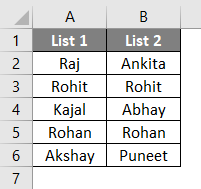
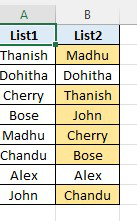
Below are two lists called List1 and List2 which we’ll compare.
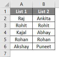
Now, we’ll insert another column called “Result” to display the result as TRUE or FALSE. If there is a match in both cells in a row, then it will show TRUE; else, it will show FALSE. We’ll use the Equal sign operator for the same.
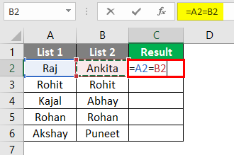
After using the above formula, the output is shown below.
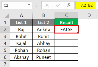
The formula is =A2=B2, which states cell A2 is compared with cell B2. A1 has “Raj”, and B1 has “Ankita”, which does not match. So, it will show FALSE in the first row of the result column. Similarly, the rest of the rows can be compared. Alternatively, we can drag the cursor from C2 to C6 to get the result automatically.
Example #2 – Match Data using Row Difference Technique
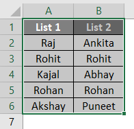
To demonstrate this technique, we’ll use the same data as above.
First of all, the entire data is selected.
Then by pressing the F5 key on the keyboard, the “Go to special” dialog box opens. Then go to Special as shown below.
Now, select “Row difference” from the options and press on OK.
Now, matching cells are in while color and unmatched cells in white and grey color as shown below.
We can highlight the row difference values for different colors as per our convenience.
Example #3 – Row Difference using IF Condition
If condition basically states if there is any match in the row. If there’s a match, the result will be “Matching” or else “Not Matching”. The formula is shown below.
After using the above formula, the output is shown below.
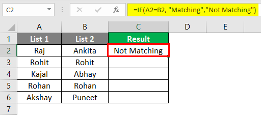
Here A2 and B2 values don’t match, so that the result will be “Not Matching”. Similarly, other rows can result with the condition, or alternatively, we can drag the cursor, and the output will come automatically as below.
Example #4 – Matching Data in case of Row Difference
This technique is not accurate always as values may be in other cells too. So, different techniques are used for the same.
Now we’ll apply the V-Lookup function to get the result in a new column.
After applying the formula, the output is shown below.
Here, the function states that B2 is being compared with values from List 1. So, the range is A2:A9. And the result can be seen as shown below.
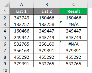
If 160466 is there in any cell in List 1 then, 160466 will be printed using V-Lookup. Similarly, the rest values can be checked. In the 2nd and 5th row, there is an error. It is because values 183258 and 356160 are not present in List 1. For that, we can apply the IFERROR function as follows. Now, the result is finally here.
Example #5 – Highlighting Matching Data
Sometimes, we feel fed up with Excel formulas. So, we can use this method to highlight all the matching data. This method is basically conditional formatting. First, we’ll have to highlight the data.
Next, we have to go to Conditional formatting > Highlight cell rules > Duplicate values as shown below.
Then a dialog box appears as below.
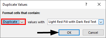
We can either choose a different color from the drop-down list or stick with the default one, as shown above. Now the result can be seen clearly below.
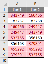
Here common values are highlighted in red color while unique values are colorless. We can color only unique values if we need to find unmatched values. For that, instead of selecting “duplicate” in the Duplicate values dialog box, we’ll select “Unique” and then press on OK.
Now, the result is shown below.
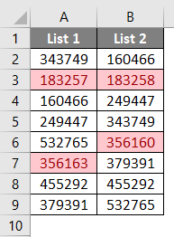
Here, only unique and unmatched values are highlighted in red.
Example #6 – Partial Matching Technique
Sometimes both lists don’t have the exact data. For example, if we have “India is a country” in List 1 and “India” in List 2, then formulas or matching techniques won’t work here. Because List 2 has partial information of List 1. In such cases, the special character “*” can be used. Below are two lists with company names with their revenue.
Here, we’ll apply V-Lookup using the special character “*” as shown below.
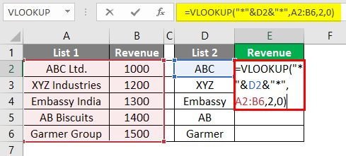
Now, we can see that 1000 is printed in cell E2. We can drag the formula till cell E6 to the result in other cells as well.
Things to Remember
- The above techniques depend on the data structure of the table.
- V-Lookup is the common formula to use when the data is not organized.
- Row by row technique works in the case of organized data.
Recommended Articles
This is a guide to Compare Two Lists in Excel. Here we discuss How to Compare Two Lists in Excel along with practical examples and a downloadable excel template. You can also go through our other suggested articles –
- Excel Compare Two Columns
- Compare Dates in Excel
- Compare Text in Excel
- Compare Two Columns in Excel for Matches
All the time there is a necessity in Excel to look at two records or two informational indexes to track down absent or matching things. As this is Excel, there is in every case more than one method for getting things done, including looking at information. From equations and Conditional Formatting to Power Query. Let’s take a look at a number of ways of contrasting two records in Excel and we will likewise take a gander at looking at whole columns of an informational collection. The following are a few distinct strategies used to look at two arrangements of a segment in Excel for matches and contrasts.
- Strategy 1: Compare Two Lists Using Equal Sign Operator.
- Strategy 2: Match Data by Using Row Difference Technique.
- Strategy 3: Match Row Difference by Using IF Condition.
- Strategy 4: Match Data Even If There is a Row Difference.
- Strategy 5: Highlight All the Matching Data utilizing Conditional Formatting.
Presently, let us talk about every one of the techniques exhaustively with a model: –
Strategy 1: Compare Two Lists Using Equal Sign Operator
We should follow the underneath moves toward looking at the two records.
- Immediately after the two columns, we must insert a new column in the next column.
- We should place the equation in cell C2 as =A2=B2.
- This equation tests whether cell A2 esteem is equivalent to cell B2. On the off chance that both the cell values are coordinated, we will come by the outcome as “TRUE” or “FALSE.”
- We will drag the recipe to cell C9 to decide on different qualities.
Any place we share similar qualities practically speaking lines, we obtain the outcome as “TRUE” or “FALSE”.
Strategy 2: Match Data by Using Row Difference Technique
You probably won’t have utilized the “Column Difference” strategy in your working environment. Be that as it may, today, we will tell you the best way to utilize this procedure to match information column by line.
- To feature non-matching cells column by line, we should choose the whole information first.
- Presently, we should press the successful easy route key “F5” to open the “Go to Special” instrument. Presently in the “Go-To” window, press the “Special” tab.
- In the following window, we should go to the “Go To Special” and pick the “Row differences” choice. Then, at that point, click on “OK.”
- We will obtain the accompanying outcome.
As we can find in the above window, it has chosen the cells any place there is a line distinction. Hence, we should fill in a variety to feature the line contrast values.
Strategy 3: Match Row Difference by Using IF Condition
How might we leave out the IF condition when we have any desire to match information column by line. In the primary model, we have by the same token “TRUE” or “FALSE.” But consider the possibility that we really want an alternate outcome rather than the default consequences of by the same token “TRUE or FALSE.” Assume we want an outcome as “Coordinating” in the event that there is no column distinction and the outcome ought to be “Not Matching” on the off chance that there is a line contrast.
- To begin with, we should open the IF condition in cell C2. Apply the logical test as A2=B2.
- Note: Logical Test=>In excel, toward the early phases of learning, it is a seriously troublesome errand to grasp the idea of consistent tests. Be that as it may, when you ace this, it will be significant expertise to your CV. As a general rule, in succession, we utilize a legitimate test to match various models also, show up at the ideal arrangement. To succeed, we have as numerous consistent equations. Go to the Formula tab and snap on the Logical Function gathering to see every one of the sensible recipes.
- We really want to apply the recipe to come by the outcome. We should drag the recipe to cell C9 to decide on different qualities.
Strategy 4: Match Data Even If There is a Row Difference
The matching information on the column distinctions system may not work continually; the value may be in various cells also. So we truly need to include different advances in these circumstances. As of now, look at the underneath data. So let us utilize our capability VLOOKUP(Note: The VLOOKUP succeed capability looks for a specific worth and returns a relating match in view of an exceptional identifier. An exceptional identifier is extraordinarily connected with every one of the records of the information base.)
Along these lines, if the data matches, we get the Name; regardless, we get the bumble regarded as #N/A. Showing mistake values doesn’t look great. So rather than showing the mistake, let us supplant them with “Not Available.” For this, utilization of the IFERROR( Note: The IFERROR capacity in Excel truly investigates a recipe for mix-ups and returns a foreordained worth rather than the goof. This returned worth can be a text, an empty string, a reasonable worth, a number, etc. The bumbles are dealt with by the capacity to consolidate “#N/A,” “#DIV/0!,” “#NAME, and so forth) capability in excel.
Strategy 5: Highlight All the Matching Data utilizing Conditional Formatting
On the off chance that you hate excel recipes, relax. We can in any case match information without the equation. For instance, utilizing straightforward restrictive formatting (Note: Conditional designing in excel helps design scope of cells in view of the satisfaction of at least one circumstance. The design to be applied can either be chosen from the different choices given in Excel or made without any preparation by the client. Contingent designing chips away at the standard “if so, then that ought to be finished.”) in excel, we can feature every one of the matching information of two records.
- We ought to first pick the data. Presently, we should go to “Home” and “Contingent Formatting” and pick “Highlight Cell Rules” > “Duplicate Values.”
- Subsequently, we can see the “Duplicate Cell Values” arranging window.
- We can pick the different design tones starting from the drop list in excel. Select the primary arranging tone and press the “OK” button.
- This will feature every one of the matching information from the two records.
- Simply for the situation, rather than featuring every one of the matching information, to feature not matching information, then, at that point, we can go to the “Duplicate Values” window and pick the choice “Unique.”
- Subsequently, it will feature every one of the non-matching qualities, as displayed beneath.