
IF function
The IF function is one of the most popular functions in Excel, and it allows you to make logical comparisons between a value and what you expect.
So an IF statement can have two results. The first result is if your comparison is True, the second if your comparison is False.
For example, =IF(C2=”Yes”,1,2) says IF(C2 = Yes, then return a 1, otherwise return a 2).

Use the IF function, one of the logical functions, to return one value if a condition is true and another value if it’s false.
IF(logical_test, value_if_true, [value_if_false])
For example:
-
=IF(A2>B2,»Over Budget»,»OK»)
-
=IF(A2=B2,B4-A4,»»)
|
Argument name |
Description |
|---|---|
|
logical_test (required) |
The condition you want to test. |
|
value_if_true (required) |
The value that you want returned if the result of logical_test is TRUE. |
|
value_if_false (optional) |
The value that you want returned if the result of logical_test is FALSE. |
Simple IF examples

-
=IF(C2=”Yes”,1,2)
In the above example, cell D2 says: IF(C2 = Yes, then return a 1, otherwise return a 2)

-
=IF(C2=1,”Yes”,”No”)
In this example, the formula in cell D2 says: IF(C2 = 1, then return Yes, otherwise return No)As you see, the IF function can be used to evaluate both text and values. It can also be used to evaluate errors. You are not limited to only checking if one thing is equal to another and returning a single result, you can also use mathematical operators and perform additional calculations depending on your criteria. You can also nest multiple IF functions together in order to perform multiple comparisons.

-
=IF(C2>B2,”Over Budget”,”Within Budget”)
In the above example, the IF function in D2 is saying IF(C2 Is Greater Than B2, then return “Over Budget”, otherwise return “Within Budget”)

-
=IF(C2>B2,C2-B2,0)
In the above illustration, instead of returning a text result, we are going to return a mathematical calculation. So the formula in E2 is saying IF(Actual is Greater than Budgeted, then Subtract the Budgeted amount from the Actual amount, otherwise return nothing).

-
=IF(E7=”Yes”,F5*0.0825,0)
In this example, the formula in F7 is saying IF(E7 = “Yes”, then calculate the Total Amount in F5 * 8.25%, otherwise no Sales Tax is due so return 0)
Note: If you are going to use text in formulas, you need to wrap the text in quotes (e.g. “Text”). The only exception to that is using TRUE or FALSE, which Excel automatically understands.
Common problems
|
Problem |
What went wrong |
|---|---|
|
0 (zero) in cell |
There was no argument for either value_if_true or value_if_False arguments. To see the right value returned, add argument text to the two arguments, or add TRUE or FALSE to the argument. |
|
#NAME? in cell |
This usually means that the formula is misspelled. |
Need more help?
You can always ask an expert in the Excel Tech Community or get support in the Answers community.

See Also
IF function — nested formulas and avoiding pitfalls
IFS function
Using IF with AND, OR and NOT functions
COUNTIF function
How to avoid broken formulas
Overview of formulas in Excel
Need more help?
When you have a lot of data in a spreadsheet it becomes quite difficult to compare the contents of two cells without just staring closely into the screen.
Moreover, if your data pans over a large number of rows, it can be quite annoying to compare data in cells that are quite far apart.
In this tutorial we will show you how to compare two cells in Excel, in different cases:
- When you want to compare for an exact match (case insensitive)
- When you want to compare for an exact match (case sensitive)
- When you want to display a defined value for a match or no match
- When you want to compare for a partial match
- When you want to compare numeric values in the cells
How to Compare Two Cells for an Exact Match (Case Insensitive)
This method is probably the quickest way to compare two cells in Excel (for equality).
The formula used in this method is really simple, involving only a comparison operator, in this case, the ‘equal to’ operator.
Say you have two values in cells B1 and B2, and you want to find out if they are an exact match or not.

Simply type the following formula to return a TRUE (if they match) or FALSE (if they don’t).
=B1=B2
Please note that this formula does not consider whether the contents of the cells are in upper or lowercase. Both are considered the same.
If the contents of both cells match exactly (irrespective of case), the formula returns a TRUE. Else, it returns a FALSE.

How to Compare Two Cells for an Exact Match (Case Sensitive)
If you want an exact match, including the case of the text, then you should use the EXACT function instead of the comparison operator.
The EXACT function takes two strings and checks for an exact match, including whether the text is in upper or lower case.
The syntax for the function is simple:
=EXACT(text1, text2)
Here, text1 and text2 are the two strings that we want to compare.
The function compares the two strings and returns a TRUE value if there is an exact match (including case), and FALSE if there isn’t.
In the following example, the EXACT function returns a FALSE, since the strings in cells B1 and B2 don’t match (although both cells have the same text, the value in B1 starts with an uppercase letter, while the one in B2 starts with a lowercase letter).

How to Display a Defined value for a Match or No Match
The above two methods simply return a TRUE or FALSE value after testing for a match.
However, someone else looking at your worksheet might not be able to understand what you mean by TRUE or FALSE.
So you might want to return a more descriptive value if there’s a match.
Moreover, you might want to display some specific text for a match in some cases.
For example, you might want to display the text ‘Winning’ if values in cells B1 and B2 are equal. If not then you can probably display “Not winning”, or something like that.
For this, you can use the IF function as follows:
=IF(B1=B2,"Winning","Not winning")
The above formula uses the IF function to compare values in B1 and B2. If the condition “B1=B2” is TRUE, the function returns the text “Winning”. If not, it returns the text “Not winning”.

For an exact match (including case), you can use the formula:
=IF(EXACT(B1,B2),"Winning","Not winning")

If you don’t necessarily need an exact match, you can also check for a partial match between two cells.
For example, you might want to see if the last few digits of a phone number or the first few digits of an ID are the same.
To compare the first n digits, you can use the following formula:
=LEFT(string1,n)=LEFT(string2,n)
So, for example, if you want to compare the first 2 digits of values in B1 and B2, then n=2, and your formula will be:
=LEFT(B1, 2) = LEFT(B2, 2)

Similarly, to compare the last n digits, you can use the following formula:
=RIGHT(string1,n)=RIGHT(string2,n)
So, for example, if you want to compare the last 3 digits of values in B1 and B2, then n=3, and your formula will be:
=RIGHT(B1, 3) = RIGHT(B2, 3)

Note: If you want an exact match of the first n digits (including case), then you can wrap an EXACT function around the LEFT or RIGHT functions as follows:
=EXACT(LEFT(B1, 2),LEFT(B2,2))

You can also compare two cells to see if the value in one of them exists in the other.
This can be achieved using wildcard characters like ‘*’ or ‘?’. For example, consider the following pair of values:

Let’s say you want to check if the two values (in B1 and B2) match partially (one of the values exists as a part of the other value).
The formula for this is a little more complex since you will need to consider cases where the first value is smaller than the second and vice-versa:
=IF(LEN(B1)<LEN(B2),IFERROR(MATCH("*"&B1&"*",B2:B2,0)>0,FALSE),IFERROR(MATCH("*"&B2&"*",B1:B1,0)>0,FALSE))

Explanation of the Formula
Let us break down this formula and analyze it part by part:
LEN(B1)<LEN(B2)
We want to know if there is a partial match between values in B1 and B2. This means, that if the string in B1 is shorter than the string in B2, then we want to know if B1 exists in B2.
Similarly, if it’s the other way round, we want to find out if the value in B2 exists in B1.
To find out which string is shorter, we simply compare the lengths of the two strings using the LEN function.
MATCH(“*”&B1&”*”,B2:B2,0)>0
If the string in B1 is shorter than that of B2, then we want to check if the string of B1 is a part of the string in B2.
The MATCH function here checks if the value in B1 exists as a part of B2 (using the asterisk wildcard).
If it does, then the MATCH function returns the position of the matching string in B2. If it does not exist in B2, then the function returns a 0.
But we just want to know whether the value exists in B2 or not. We don’t really care about the position. So, we simply check if the value returned is more than 0.
If it is, that means that the value in B1 is a part of the value in B2. We got a partial match.
The only problem is that if there is no match, the MATCH function returns an #N/A error. To keep this in check, we can simply wrap an IFERROR function around this formula, like this:
IFERROR(MATCH(“*”&B1&”*”,B2:B2,0)>0,FALSE)
So now if the value in B1 does not exist in B2, the IFERROR function simply returns a FALSE.
In the same way, if the string in B2 is shorter than that of B1, then we want to check the other way round.
We simply exchange cell references B1 and B2, so the third parameter (of the main IF function) is specified as:
IFERROR(MATCH(“*”&B2&”*”,B1:B1,0)>0,FALSE)
To sum up, in the above formula, we simply use the IF function to compare LEN(B1) and LEN(B2). If the string in B1 is shorter, the function returns IFERROR(MATCH(“*”&B1&”*”,B2:B2,0)>0,FALSE).
Otherwise, it returns IFERROR(MATCH(“*”&B2&”*”,B1:B1,0)>0,FALSE)
Let us try this on a few sample pairs of strings to see if the formula actually works in all cases:

As we can see, the formula compares the two values in each column and returns a TRUE whenever there is a partial match, and a FALSE when there’s no match.
How to Compare Two Cells to Find the Larger or Smaller Number
Finally, let us see a case where you have numeric values in two different cells and you want to compare them to see if one of them is larger than the other.
For example, the following dataset contains pairs of values in rows 1 and 2, and we want to find out which value is larger.

The formula you can use is as follows:
=IF(B1>B2,B1,B2)

If you just want to know if the value in B2 is larger than the one in B1, then your formula will be:
=B2>B1

In this tutorial, we showed you how to compare two cells in a variety of cases.
We tried to cover as many comparison possibilities as we could think of. We hope from the cases we mentioned here you were able to find what you needed.
Other Excel tutorials you may also find helpful:
- How to Compare Two Columns in Excel (using VLOOKUP & IF)
- Find the Closest Match in Excel (Nearest Value) – Easy Formula
- How to Paste in a Filtered Column Skipping the Hidden Cells
- How to Compare Dates in Excel (Greater/Less Than, Mismatches)
- How to Compare Two Excel Sheets (for differences)
- How to Hide Rows based on Cell Value in Excel
- ‘Does Not Equal’ Operator in Excel (Examples)
Watch Video – Compare two Columns in Excel for matches and differences
The one query that I get a lot is – ‘how to compare two columns in Excel?’.
This can be done in many different ways, and the method to use will depend on the data structure and what the user wants from it.
For example, you may want to compare two columns and find or highlight all the matching data points (that are in both the columns), or only the differences (where a data point is in one column and not in the other), etc.
Since I get asked about this so much, I decided to write this massive tutorial with an intent to cover most (if not all) possible scenarios.
If you find this useful, do pass it on to other Excel users.
Note that the techniques to compare columns shown in this tutorial are not the only ones.
Based on your dataset, you may need to change or adjust the method. However, the basic principles would remain the same.
If you think there is something that can be added to this tutorial, let me know in the comments section
Compare Two Columns For Exact Row Match
This one is the simplest form of comparison. In this case, you need to do a row by row comparison and identify which rows have the same data and which ones does not.
Example: Compare Cells in the Same Row
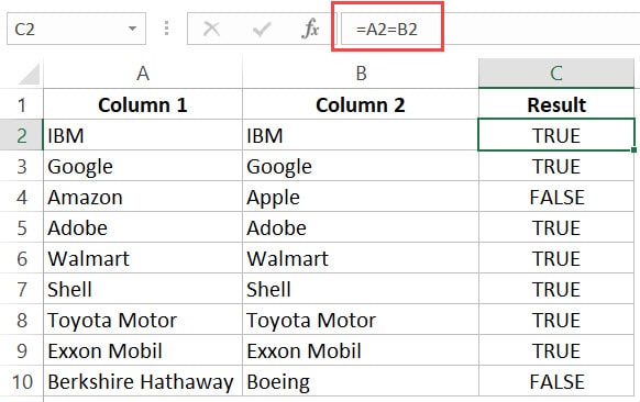
Below is a data set where I need to check whether the name in column A is the same in column B or not.
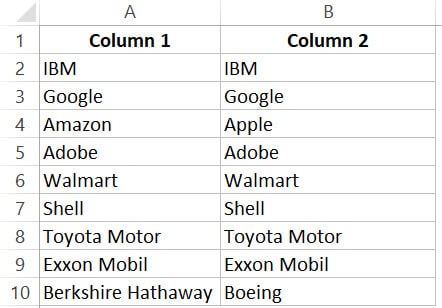
If there is a match, I need the result as “TRUE”, and if doesn’t match, then I need the result as “FALSE”.
The below formula would do this:
=A2=B2
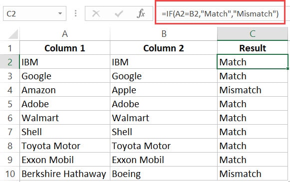
Example: Compare Cells in the Same Row (using IF formula)
If you want to get a more descriptive result, you can use a simple IF formula to return “Match” when the names are the same and “Mismatch” when the names are different.
=IF(A2=B2,"Match","Mismatch")
Note: In case you want to make the comparison case sensitive, use the following IF formula:
=IF(EXACT(A2,B2),"Match","Mismatch")
With the above formula, ‘IBM’ and ‘ibm’ would be considered two different names and the above formula would return ‘Mismatch’.
Example: Highlight Rows with Matching Data
If you want to highlight the rows that have matching data (instead of getting the result in a separate column), you can do that by using Conditional Formatting.
Here are the steps to do this:
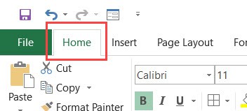
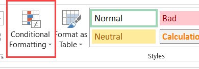
- Select the entire dataset.
- Click the ‘Home’ tab.

- In the Styles group, click on the ‘Conditional Formatting’ option.

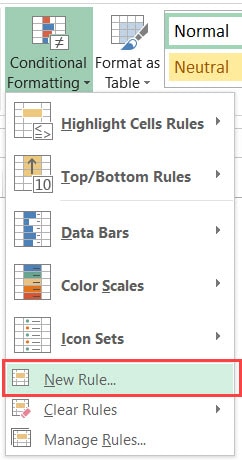
- From the drop-down, click on ‘New Rule’.

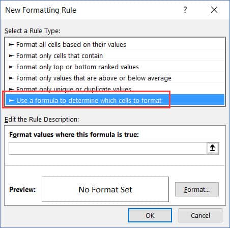
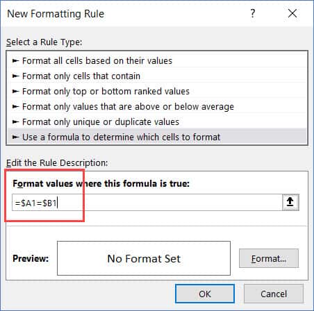
- In the ‘New Formatting Rule’ dialog box, click on the ‘Use a formula to determine which cells to format’.

- In the formula field, enter the formula: =$A1=$B1
- Click the Format button and specify the format you want to apply to the matching cells.
- Click OK.
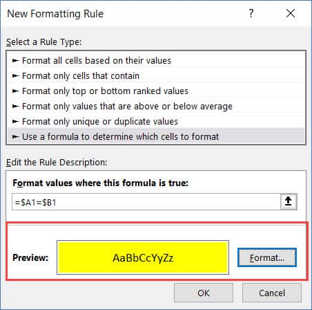
This will highlight all the cells where the names are the same in each row.
Compare Two Columns and Highlight Matches
If you want to compare two columns and highlight matching data, you can use the duplicate functionality in conditional formatting.
Note that this is different than what we have seen when comparing each row. In this case, we will not be doing a row by row comparison.
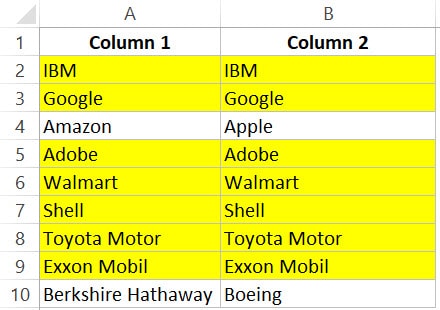
Example: Compare Two Columns and Highlight Matching Data
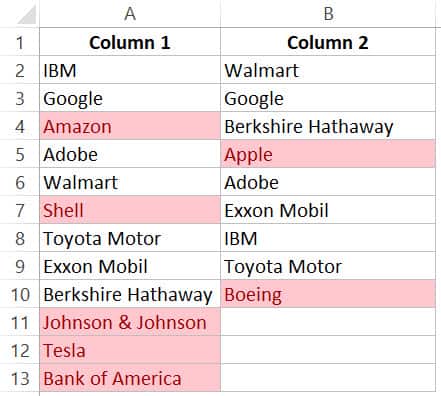
Often, you’ll get datasets where there are matches, but these may not be in the same row.
Something as shown below:
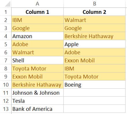
Note that the list in column A is bigger than the one in B. Also some names are there in both the lists, but not in the same row (such as IBM, Adobe, Walmart).
If you want to highlight all the matching company names, you can do that using conditional formatting.
Here are the steps to do this:
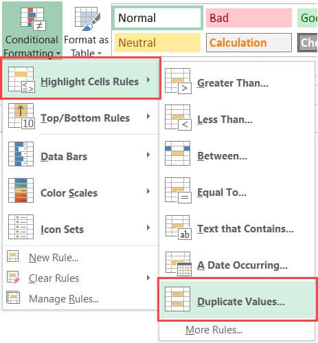
- Select the entire data set.
- Click the Home tab.
- In the Styles group, click on the ‘Conditional Formatting’ option.
- Hover the cursor on the Highlight Cell Rules option.
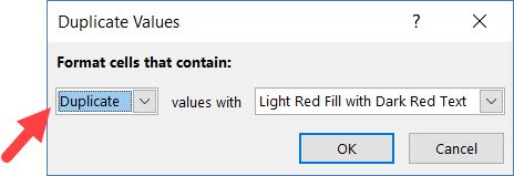
- Click on Duplicate Values.

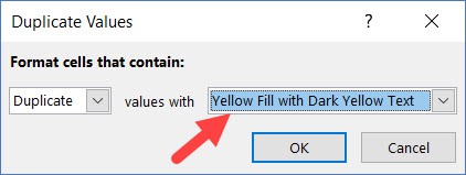
- In the Duplicate Values dialog box, make sure ‘Duplicate’ is selected.

- Specify the formatting.

- Click OK.
The above steps would give you the result as shown below.
Note: Conditional Formatting duplicate rule is not case sensitive. So ‘Apple’ and ‘apple’ are considered the same and would be highlighted as duplicates.
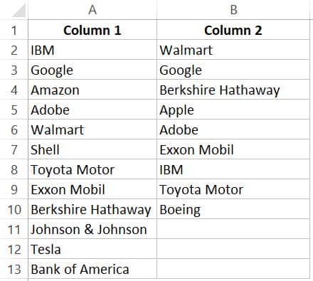
Example: Compare Two Columns and Highlight Mismatched Data
In case you want to highlight the names which are present in one list and not the other, you can use the conditional formatting for this too.
- Select the entire data set.
- Click the Home tab.
- In the Styles group, click on the ‘Conditional Formatting’ option.
- Hover the cursor on the Highlight Cell Rules option.
- Click on Duplicate Values.
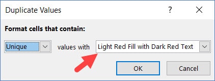
- In the Duplicate Values dialog box, make sure ‘Unique’ is selected.

- Specify the formatting.
- Click OK.
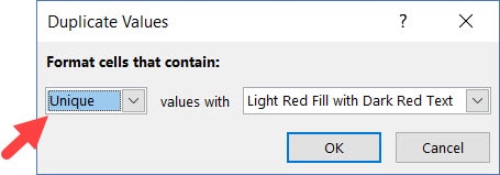
This will give you the result as shown below. It highlights all the cells that have a name that is not present on the other list.
Compare Two Columns and Find Missing Data Points
If you want to identify whether a data point from one list is present in the other list, you need to use the lookup formulas.
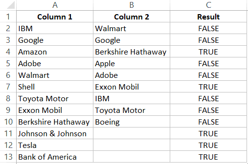
Suppose you have a dataset as shown below and you want to identify companies that are present in column A but not in Column B,
To do this, I can use the following VLOOKUP formula.
=ISERROR(VLOOKUP(A2,$B$2:$B$10,1,0))
This formula uses the VLOOKUP function to check whether a company name in A is present in column B or not. If it is present, it will return that name from column B, else it will return a #N/A error.
These names which return the #N/A error are the ones that are missing in Column B.
ISERROR function would return TRUE if there is the VLOOKUP result is an error and FALSE if it isn’t an error.
If you want to get a list of all the names where there is no match, you can filter the result column to get all cells with TRUE.
You can also use the MATCH function to do the same;
=NOT(ISNUMBER(MATCH(A2,$B$2:$B$10,0)))
Note: Personally, I prefer using the Match function (or the combination of INDEX/MATCH) instead of VLOOKUP. I find it more flexible and powerful. You can read the difference between Vlookup and Index/Match here.
Compare Two Columns and Pull the Matching Data
If you have two datasets and you want to compare items in one list to the other and fetch the matching data point, you need to use the lookup formulas.
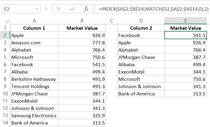
Example: Pull the Matching Data (Exact)
For example, in the below list, I want to fetch the market valuation value for column 2. To do this, I need to look up that value in column 1 and then fetch the corresponding market valuation value.
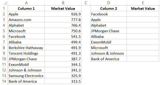
Below is the formula that will do this:
=VLOOKUP(D2,$A$2:$B$14,2,0)
or
=INDEX($A$2:$B$14,MATCH(D2,$A$2:$A$14,0),2)
Example: Pull the Matching Data (Partial)
In case you get a dataset where there is a minor difference in the names in the two columns, using the above-shown lookup formulas is not going to work.
These lookup formulas need an exact match to give the right result. There is an approximate match option in VLOOKUP or MATCH function, but that can’t be used here.
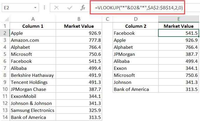
Suppose you have the data set as shown below. Note that there are names that are not complete in Column 2 (such as JPMorgan instead of JPMorgan Chase and Exxon instead of ExxonMobil).
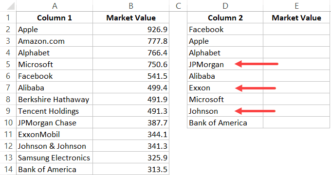
In such a case, you can use a partial lookup by using wildcard characters.
The following formula will give is the right result in this case:
=VLOOKUP("*"&D2&"*",$A$2:$B$14,2,0)
or
=INDEX($A$2:$B$14,MATCH("*"&D2&"*",$A$2:$A$14,0),2)
In the above example, the asterisk (*) is a wildcard character that can represent any number of characters. When the lookup value is flanked with it on both sides, any value in Column 1 which contains the lookup value in Column 2 would be considered as a match.
For example, *Exxon* would be a match for ExxonMobil (as * can represent any number of characters).
You May Also Like the Following Excel Tips & Tutorials:
- How to Compare Two Excel Sheets (for differences)
- How to Highlight Blank Cells in Excel.
- How to Compare Text in Excel (Easy Formulas)
- Highlight EVERY Other ROW in Excel.
- Excel Advanced Filter: A Complete Guide with Examples.
- Highlight Rows Based on a Cell Value in Excel
- How to Compare Dates in Excel (Greater/Less Than, Mismatches)
This post will guide you how to check if the values of multiple cells are equal with a formula in Excel. How do I verify that multiple cellsare the same in Excel. How to compare three or more cells in Excel to see if they are the same with a formula.
Table of Contents
- Check If Multiple Cells are Equal
- Related Functions
Assuming that you have a list of data in range A1:C1, and you want to compare if these cells are equal, if so, then return True, otherwise, return False. How to achieve it.
You need to create an Excel array formula based on the AND function and the EXACT function. Just like this:
=AND(EXACT(A1:C1,A1))
Type this formula into a blank cell, and press Ctrl +Shift +Enter shortcuts in your keyboard.
There is another formula based on the COUNTIF function to achieve the same result. Like this:
=COUNTIF(A1:C1,A1)=3
- Excel AND function
The Excel AND function returns TRUE if all of arguments are TRUE, and it returns FALSE if any of arguments are FALSE.The syntax of the AND function is as below:= AND (condition1,[condition2],…) … - Excel COUNTIF function
The Excel COUNTIF function will count the number of cells in a range that meet a given criteria. This function can be used to count the different kinds of cells with number, date, text values, blank, non-blanks, or containing specific characters.etc.= COUNTIF (range, criteria)… - Excel EXACT function
The Excel EXACT function compares if two text strings are the same and returns TRUE if they are the same, Or, it will return FALSE.The syntax of the EXACT function is as below:= EXACT (text1,text2)…
Two columns in excel are compared when their entries are studied for similarities and differences. The similarities are the data values that exist in the same row of both the compared columns. In contrast, the differences are those values that exist in only one of these columns.
For example, for a specific month, a table displays the following information:
- Column A lists the names of the employees who took three consecutive leaves.
- Column B lists the names of the employees who took two consecutive leaves.
Since the data pertains to the same organization, there can be a similarity or a difference within the given set of values. The same is explained as follows:
- A similarity or a match (column A is equal to column B) implies employees who took both three and two continuous leaves.
- A difference (column A is not equal to column B) implies employees who took either three or two continuous leaves.
It is difficult to scan through the data to track the matches and the differences manually. Hence, there are techniques which can be followed to compare 2 columns of an excel worksheet.
Table of contents
- Compare two Columns in Excel
- How to Compare two Columns in Excel? (Top 4 Methods)
- #1 – Compare Using Simple Formulae
- #2 – Compare 2 Columns Using the IF Formula
- #3 – Compare Using the EXACT Formula
- #4 – Compare 2 Excel Columns Using Conditional Formatting
- The Properties of the Comparison Methods
- Frequently Asked Questions
- Recommended Articles
- How to Compare two Columns in Excel? (Top 4 Methods)
How to Compare two Columns in Excel? (Top 4 Methods)
The top four methods to compare 2 columns are listed as follows:
- Method #1–Compare using simple formulae
- Method #2–Compare using the IF formula
- Method #3–Compare using the EXACT formula
- Method #4–Compare using conditional formatting
Let us understand these methods with the help of examples.
You can download this Compare Two Columns Excel Template here – Compare Two Columns Excel Template
#1 – Compare Using Simple Formulae
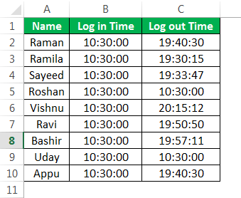
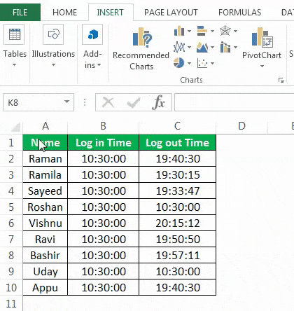
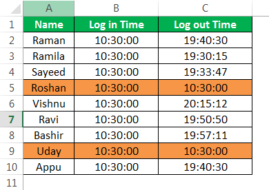
The following table shows the names of the employees of an organization in column A. Columns B and C display their log-in and the log-out times respectively.
We want to compare two excel columns B and C to find out the employees who forgot to logout from the office. The official timings are 10:30 a.m.-7:30 p.m. Use the formula method for comparison.
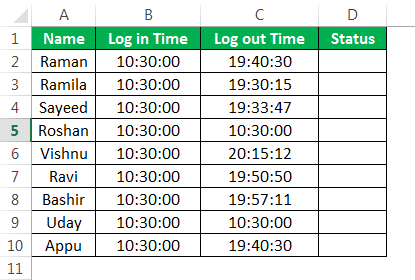
For the given data, if the log-in time is equal to the log-out time, we assume that the employee has forgotten to logout.
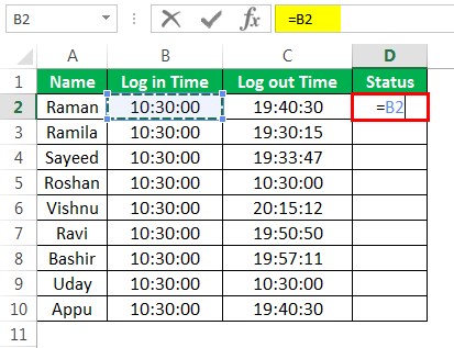
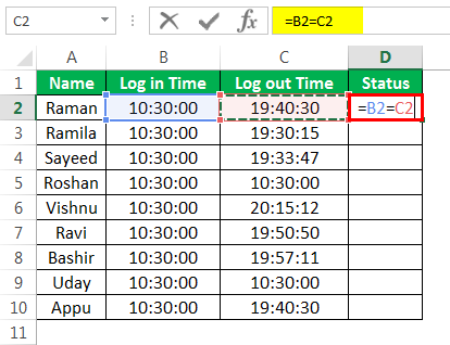
The steps to compare two columns in excel with the help of the comparison operator “equal to” (=) are listed as follows:
- In cell D2, enter the symbol “=” followed by selecting the cell B2.

- Enter the symbol “=” again, followed by selecting the cell C2.

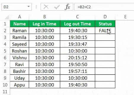
- Press the “Enter” key. It returns “false.” This implies that the value in cell B2 is not equal to that of cell C2.

- Drag or copy-paste the formula to the remaining cells. The output is either “true” or “false,” as shown in the following image.
If the value in column B is equal to that of column C, the result is “true,” else “false.” The cells D5 and D9 show the output “true.”
Hence, Roshan and Uday forgot to logout from the office.

#2 – Compare 2 Columns Using the IF Formula
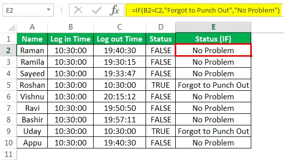
Working on the data of example #1, we want the following results:
- “Forgot to punch out,” if the employee forgets to logout
- “No problem,” if the employee logs out
Use the IF functionIF function in Excel evaluates whether a given condition is met and returns a value depending on whether the result is “true” or “false”. It is a conditional function of Excel, which returns the result based on the fulfillment or non-fulfillment of the given criteria.
read more to compare the columns B and C.
We apply the following formula.
“=IF(B2=C2,“Forgot to Punch Out”,“No Problem”)”
If the value in column B is equal to that of column C, the result is “true,” otherwise “false.” For every “true” value, the formula returns “forgot to punch out.” Likewise, it returns “no problem” for every “false” value.
The output is shown in column E of the following image.
Hence, Roshan and Uday are the only two employees who have forgotten to logout from the office.
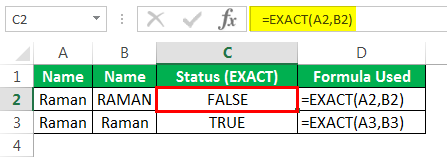
#3 – Compare Using the EXACT Formula
Working on the data of example #1, we want to compare the two excel columns B and C with the help of the EXACT functionThe exact function is a logical function in excel used to compare two strings or data with each other, and it gives us the result whether the both data are an exact match or not. This function is a logical function, so it provides true or false as a result.read more.
We apply the following formula.
“=EXACT(B2,C2)”
If the value in column B is equal to that of column C, the formula returns “true,” otherwise “false.” The output is shown in column F of the following image.
Hence, the entries of columns B and C are identical for Roshan and Uday.
Note: The EXACT function is case-sensitive.

We have written the name “Raman” in columns A and B with different casing. We apply the following formula.
“=EXACT(A2,B2)”
The formula returns “false” when the casing of cell A2 is different from that of cell B2. Likewise, it returns “true” if the casing in columns A and B is the same.
The output is shown in column C of the following image.
#4 – Compare 2 Excel Columns Using Conditional Formatting
Working on the data of example #1, we want to highlight those entries that are identical in columns B and C. Use the conditional formattingConditional formatting is a technique in Excel that allows us to format cells in a worksheet based on certain conditions. It can be found in the styles section of the Home tab.read more feature.
Step 1: Select the entire data. In the Home tab, click the “conditional formatting” drop-down under the “styles” section. Select “new rule.”
Step 2: The “new formatting rule” window appears. Under “select a rule type,” choose the option “use a formula to determine which cells to format.”
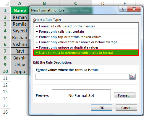
Step 3: Enter the formula “$B2=$C2” under “edit the rule description.”
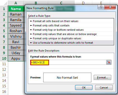
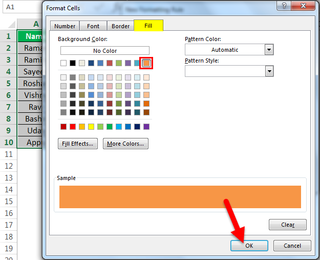
Step 4: Click “format.” In the “format cells” window, select the color to highlight the identical entries. Click “Ok.” Click “Ok” again in the “new formatting rule” window.
Step 5: The matches of columns B and C are highlighted, as shown in the following image.
Hence, the entries of columns B and C are identical for Roshan and Uday.
The Properties of the Comparison Methods
The features of the comparison methods discussed are listed as follows:
- The outcomes of the IF function can be modified according to the requirement of the user.
- The EXACT function returns “false” for two same values having different casing.
- The simplest technique to compare two excel columns is by using the comparison operator “equal to” (method #1).
Note: The comparison method to be used depends on the data structure and the kind of output required.
Frequently Asked Questions
1. What does it mean to compare two columns and how is it done in Excel?
The comparison of two data columns helps find the similarities and the differences. In case of similarity, a value exists in the same row of both the columns. In contrast, a difference is a deviation of one value from the other.
To compare two excel columns, the easiest approach is listed as follows:
a. Enter the following formula.
“=cell1=cell2”
The “cell1” is a cell containing a data value in the first column. The “cell2” is a cell containing a data value in the second column. Both “cell1” and “cell2” are in the same row.
b. Press the “Enter” key.
The formula returns “true” or “false” depending on whether the value exists in both the compared columns or not.
2. How to highlight the different values of two columns without using the formula in Excel?
Let us compare the following 2 columns consisting of names in the mentioned sequence:
• Column A contains Jack, Adam, Elizabeth, Betty, and Veronica.
• Column B contains Robert, Peter, Elizabeth, Henry, and Veronica.
The steps to highlight the different values without using the formula are listed as follows:
a. Select columns A and B.
b. In the Home tab, click “find and select” drop-down under the “editing” group. Choose “go to special.”
c. In the “go to special” window, select “row differences.” Click “Ok.”
The names Robert, Peter, and Henry of column B are highlighted. These cells can be colored using the “fill color” property of Excel.
3. How to compare multiple columns in Excel?
Let us compare the following columns consisting of numbers in the mentioned sequence:
• Column A contains 3, 49, 20, 22, and 86 in the range A1:A5.
• Column B contains 29, 49, 38, 21, and 86 in the range B1:B5.
• Column C contains 12, 49, 56, 24, and 86 in the range C1:C5.
The steps to compare columns A, B, and C are stated as follows:
a. Enter the following formula in cell D1. “IF(COUNTIF($A1:$C5,$A1)=3,“full match”,“”)”
b. Press the “Enter” key.
c. Drag or copy-paste the formula to the remaining cells.
Since we are comparing three excel columns, we enter the number 3 in the formula. The formula returns “full match” in cells D2 and D5. It returns an empty string in the cells D1, D3, and D4.
Hence, the numbers 49 and 86 appear in the respective rows 2 and 5 of all the three columns.
Recommended Articles
This has been a guide to compare two columns in Excel. Here we discussed the top 4 methods to compare 2 columns in Excel, 1) the operator “equal to”, 2) IF function, 3) EXACT formula, and 4) conditional formatting. We also went through some practical examples. You can download the Excel template from the website. For more on Excel, take a look at the following articles-
- Freeze Columns in ExcelFreezing columns in excel fixes or locks them so that they remain visible while scrolling through the database. A frozen column does not move with the movement of the remaining columns.read more
- Excel Rows to ColumnsRows can be transposed to columns by using paste special method and the data can be linked to the original data by simply selecting ‘Paste Link’ form the paste special dialog box. It could also be done by using INDIRECT formula and ADDRESS functions.read more
- Count Only Unique Values in ExcelIn Excel, there are two ways to count values: 1) using the Sum and Countif function, and 2) using the SUMPRODUCT and Countif function.read more
- Advanced Filter in ExcelThe advanced filter is different from the auto filter in Excel. This feature is not like a button that one can use with a single click of the mouse. To use an advanced filter, we have to define criteria for the auto filter and then click on the “Data” tab. Then, in the advanced section for the advanced filter, we will fill our criteria for the data.read more