
Содержание
- Команды, функции и состояния Excel
- Команды
- Функции
- Функции листа
- Функции листа макросов
- Состояния Excel
- Excel Commands, Functions, and States
- Commands
- Functions
- Worksheet Functions
- Macro-Sheet Functions
- Excel States
- Excel Commands
- List of Top 10 Commands in Excel
- #1 VLOOKUP Function to Fetch Data
- #2 IF Condition to Do Logical Test
- #3 CONCATENATE Function to Combine Two or More Values
- #4 Count Only Numerical Values
- #5 Count All Values
- #6 Count Based on Condition
- #7 Count Number of Characters in the Cell
- #8 Convert Negative Value to Positive Value
- #9 Convert All Characters to UPPERCASE Values
- #10 Find Maximum and Minimum Values
- Things to Remember
- Recommended Articles
Команды, функции и состояния Excel
Относится к: Excel 2013 | Office 2013 | Visual Studio
Microsoft Excel распознает два очень разные типа дополнительных функциональных возможностей: команды и функции.
Команды
В Excel команды имеют следующие свойства:
Выполняют действия так же, как и пользователи.
Могут делать все, что может пользователь (в зависимости от ограничений используемого интерфейса), например изменять параметры Excel, открывать, закрывать и редактировать документы, выполнять пересчеты и т. д.
Могут вызываться, когда происходят определенные обрабатываемые события.
Могут отображать диалоговые окна и взаимодействовать с пользователем.
Могут вызываться при выполнении определенных действиях с объектом, например щелчке левой кнопкой мыши.
Они никогда не вызываются программой Excel во время пересчета.
Они не вызываются функциями во время пересчета.
Функции
В Excel функции имеют следующие свойства:
Как правило, принимают аргументы и всегда возвращают результат.
Могут вводиться в одну или несколько ячеек в составе формулы Excel.
Могут использоваться в определениях определенных имен.
Могут использоваться в выражениях лимитов и порогов условного форматирования.
Могут вызываться командами.
Не могут вызывать команды.
����� ����, Excel ��������� ���������������� ������� ����� � ���������������� �������, ��������������� ��� ������ �� ������ ��������. Использование функций листа макросов не ограничено только листами макросов: их можно использовать там же, где и обычные функции листа.
Функции листа
В Excel функции листа имеют следующие свойства:
Не имеют доступа к информационным функциям листа макросов.
Не могут получать значения невычисленных ячеек.
Могут записываться и регистрироваться как потокобезопасные, начиная с Excel 2007.
Функции листа макросов
В Excel функции листа макросов имеют следующие свойства:
Имеют доступ к информационным функциям листа макросов.
Могут получать значения невычисленных ячеек, в том числе значения вызывающих ячеек.
Не считаются потокобезопасными, начиная с Excel 2007.
Excel обрабатывает функции UDF Microsoft Visual Basic для приложений как функции листа макросов, в том плане, что они имеют доступ к информации рабочей области и значению невычисленных ячеек, и не считаются потокобезопасными, начиная с Excel 2007.
Состояния Excel
Excel может находится в одном из нескольких состояний в любое время в зависимости от действий пользователя, внешнего процесса, обработанного события, запустившего макрос, или запланированного события, такого как Автосохранение.
Ниже описаны возможные состояния.
Состояние готовности: Команды или макросы не выполняются. Диалоговые окна не отображаются. Ячейки не редактируются, пользователь не выполняет операцию вырезания, копирования или вставки. Внедренные объекты не активированы.
Режим правки: пользователь начал вводить допустимые символы в незаблокированную или незащищенную ячейку, или нажал клавишу F2 для одной или нескольких незаблокированных или незащищенных ячеек.
Режим вырезания/копирования и вставки: пользователя вырезал или скопировал ячейку или ряд ячеек и еще не вставил их или вставил с помощью диалогового окна «Специальная вставка», позволяющего выполнять несколько операций вставки.
Режим указания: пользователь редактирует формулу и выбирает ячейки, адреса которых будут добавлены в редактируемую формулу.
Пользователь открывает встроенное диалоговое окно.
Пользователь инициирует пересчет.
Пользователь выполняет команду.
Excel выполняет операцию Автосохранение.
Источник
Excel Commands, Functions, and States
Applies to: Excel 2013 | Office 2013 | Visual Studio
Microsoft Excel recognizes two very different types of added functionality: commands and functions.
Commands
In Excel, commands have the following characteristics:
They perform actions in the same way that users do.
They can do anything a user can do (subject to the limits of the interface used), such as altering Excel settings, opening, closing, and editing documents, initiating recalculations, and so on.
They can be set up to be called when certain trapped events occur.
They can display dialog boxes and interact with the user.
They can be linked to control objects so that they are called when some action is taken on that object, such as left-clicking.
They are never called by Excel during a recalculation.
They cannot be called by functions during a recalculation.
Functions
Functions in Excel do the following:
They usually take arguments and always return a result.
They can be entered into one or more cells as part of an Excel formula.
They can be used in defined name definitions.
They can be used in conditional formatting limit and threshold expressions.
They can be called by commands.
They cannot call commands.
Excel makes a further distinction between user-defined worksheet functions and user-defined functions that are designed to work on macro sheets. Excel does not limit user-defined macro sheet functions only to being used on macro sheets: these functions can be used anywhere a normal worksheet function can be used.
Worksheet Functions
The following is true of Excel worksheet functions:
They cannot access macro sheet information functions.
They cannot obtain the values of uncalculated cells.
They can be written and registered as thread-safe starting in Excel 2007.
Macro-Sheet Functions
The following is true of Excel macro-sheet functions:
They can access macro sheet information functions.
They can obtain the values of uncalculated cells including the values of the calling cells.
They are not considered thread safe starting in Excel 2007.
How Excel treats a user-defined function (UDF), what it permits the function to do, and how it recalculates the function are all determined when you register the function. If a function is registered as a worksheet function but tries to do something that only a macro-sheet function can do, the operation fails. Starting in Excel 2007, if a worksheet function registered as thread safe tries to call a macro sheet function, again, the operation fails.
Excel treats Microsoft Visual Basic for Applications (VBA) UDFs as macro sheet-equivalent functions, in that they can access workspace information and the value of uncalculated cells, and they are not considered as thread safe starting in Excel 2007.
Excel States
Excel can be in one of a number of states at any given time depending on the actions of the user, an external process, a trapped event running a macro, or a timed Excel housekeeping event such as Autosave.
The states that the user experiences are as follows:
Ready state: No commands or macros are being run. No dialog boxes are being displayed. No cells are being edited and the user is not in the middle of a cut/copy and paste operation. No embedded object has focus.
Edit mode: The user has started to type valid input characters into an unlocked or unprotected cell, or has pressed F2 on one or more unlocked or unprotected cells.
Cut/copy and paste mode: The user has cut or copied a cell or range of cells and has not yet pasted them, or has pasted them using the paste-special dialog box, which enables multiple paste operations.
Point mode: The user is editing a formula and is selecting cells whose addresses are added to the formula being edited.
The user can clear the edit, point, and cut/copy modes by pressing the ESC key, which returns Excel to its ready state. Other events can clear these states, such as the following:
The user opens a built-in dialog box.
The user initiates a recalculation.
The user runs a command.
Excel performs an Autosave operation.
A timer event is trapped.
The last example is of importance to add-in developers. You should consider the impact of the normal usability of Excel where frequent timer event traps are being set and executed. When this is an important part of your add-in’s functionality, you should provide users with an easily accessible way of suspending it, so that they can cut/copy and paste normally when they need to.
Источник
Excel Commands


List of Top 10 Commands in Excel
Whether in engineering, medicine, chemistry, or any field, an Excel spreadsheet is the common tool for data maintenance. Some of them use it to maintain their database and others use this tool as a weapon to turn fortune for the respective companies they are working on. So, you, too, can turn things around for yourself by learning some of the most useful Excel commands.
Table of contents
#1 VLOOKUP Function to Fetch Data
The data in multiple sheets are common in many offices, but fetching the data from one worksheet to another and from one workbook to another is a challenge for beginners in Excel.
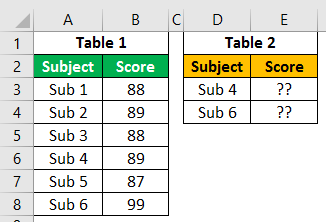
In table 1, we have the subject list and their respective scores, and in table 2, we have some subject names, but we do not have scores for them. So, using these subject names in table 2, we need to fetch the data from table 1.
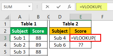
- First, let us open the VLOOKUP function in the E2 cell.
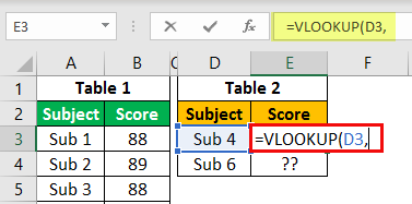
Then, select the LOOKUP value as a D3 cell.
Next, we must select the table array as A3 to B8 and press the F4 key to make them an absolute reference.
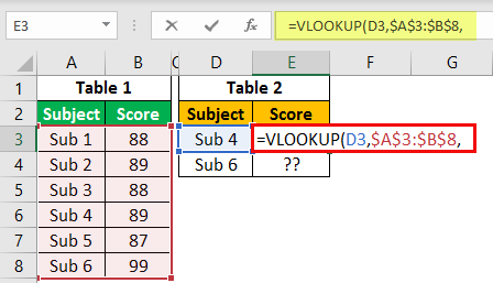
Column Index Number is from the selected table array from which column you need to fetch the data. So, in this case, from the second column, we need to bring the data.
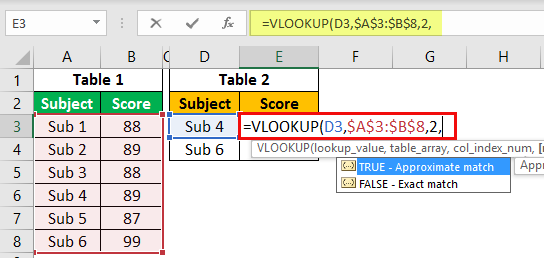
For the last argument range, LOOKUP, we must select FALSE as the option, or else we can enter.

Close the bracket and press the Enter key to get the score of Sub 4. Also, copy the formula and paste it to the below cell.
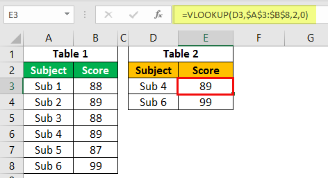
You have learned a formula to fetch values from different tables based on a LOOKUP value.
#2 IF Condition to Do Logical Test
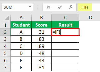
The Excel IF condition can be your friend in many situations because of its ability to conduct logical tests. For example, assume you want to test the scores of students and give the result. Below is the data for your reference.

In the above table, we have students’ scores from the examination. So we need to arrive at the result as either “PASS” or “FAIL” based on these scores. So to reach these results criteria, if the score is >=35, the result should be “PASS” or else “FAIL.”
- We must first open the IF condition in the C2 cell.
- The first argument is logical to test.So, in this example, we need to do the logical test of whether the score is >=35, select the score cell B2, and apply the logical test as B2 >= 35.
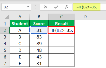
- The next argument is value if true. If the applied logical test is “TRUE,” what is the value we need? If the logical test is “TRUE,” we need the result as “Pass.”
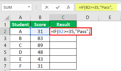
- So, the final part is value if false.If the applied logical test is “FALSE,” then we need the result as “Fail.”
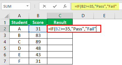
- Now, close the bracket, and we also need to fill the formula to the remaining cells.
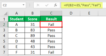
So, students A and F scored less than 35. Therefore, the result has arrived as “FAIL.”
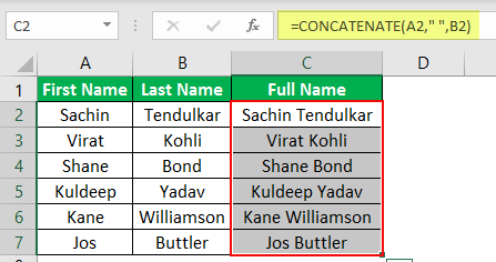
#3 CONCATENATE Function to Combine Two or More Values

- First, we need to open the CONCATENATE function in the C2 cell.
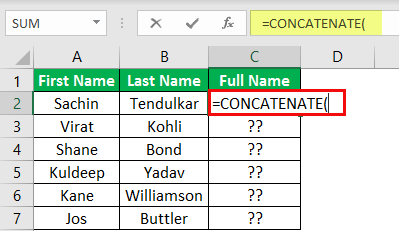
- For the first argument, “Text 1,“ select the “First Name” cell, and for “Text 2,” choose the “Last Name” cell.
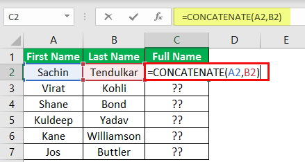
- Then, we need to apply the formula to all the cells to get the full name.

- If you want space as the “First Name” and “Last Name” separator, we can use the space character in double-quotes after selecting the first name.
#4 Count Only Numerical Values
If we want to count only numerical values from the range, you need to use the COUNT function in Excel. Take a look at the below data.
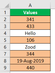
From the above table, we need to count only numerical values. For this, we can use the COUNT function.
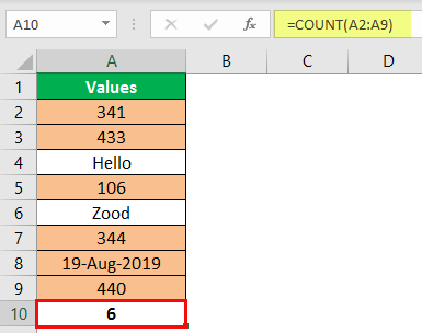
The result of the COUNT function is 6. The total count of cells is 8, but we have got the count of numerical values as 6. In cells A4 and A6, we have text values, but in cell A8, we have date values. The Excel COUNT function treats the date also as a numerical value only.
Note: “Date” and “Time” values are numerical values if the formatting is correct. Otherwise, they will be treated as “text” values.
#5 Count All Values

We got the count as 8 because the COUNTA function has counted all the cell values.
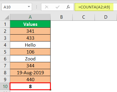
Note: Both the COUNT and COUNTA functions ignore blank cells.
#6 Count Based on Condition
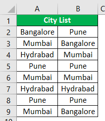
From this “City List,” if we want to count how many times “Bangalore” city is mentioned, we must open the COUNTIF function.

The first argument is “RANGE,” so we need to select the range of values from A2 to B9.
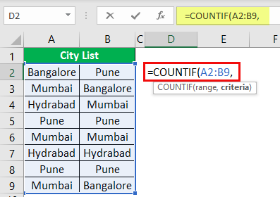
The second argument is “Criteria,” i.e., what you want to count, i.e., “Bangalore.
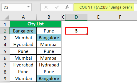
Bangalore has appeared three times in the range A2 to B9, so the COUNTIF function returns 3 as the count.
#7 Count Number of Characters in the Cell
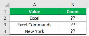
“Excel” has 5 characters, so the result is 5.
Note: Space is also considered as one character.
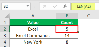
#8 Convert Negative Value to Positive Value
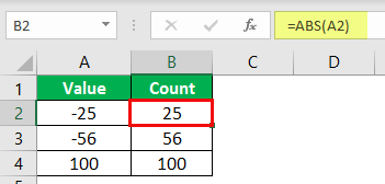
#9 Convert All Characters to UPPERCASE Values
And if we want to convert all the text values to LOWERCASE values, then use the LOWER formula.
#10 Find Maximum and Minimum Values

Things to Remember
- These are some of the important formulas/commands in excel which are used regularly.
- We can also use these functions at the advanced level.
- There are more advanced formulas in Excel which come under advanced level courses.
- Space is considered one character.
Recommended Articles
This article is a guide to Excel Commands. Here, we discuss the top 10 commands in Excel, examples, and a downloadable template. You may learn more about Excel from the following articles: –
Источник
List of Top 10 Commands in Excel
Whether in engineering, medicine, chemistry, or any field, an Excel spreadsheet is the common tool for data maintenance. Some of them use it to maintain their database and others use this tool as a weapon to turn fortune for the respective companies they are working on. So, you, too, can turn things around for yourself by learning some of the most useful Excel commands.
Table of contents
- List of Top 10 Commands in Excel
- #1 VLOOKUP Function to Fetch Data
- #2 IF Condition to Do Logical Test
- #3 CONCATENATE Function to Combine Two or More Values
- #4 Count Only Numerical Values
- #5 Count All Values
- #6 Count Based on Condition
- #7 Count Number of Characters in the Cell
- #8 Convert Negative Value to Positive Value
- #9 Convert All Characters to UPPERCASE Values
- #10 Find Maximum and Minimum Values
- Things to Remember
- Recommended Articles
You can download this Commands in Excel Template here – Commands in Excel Template
#1 VLOOKUP Function to Fetch Data
The data in multiple sheets are common in many offices, but fetching the data from one worksheet to another and from one workbook to another is a challenge for beginners in Excel.
If you have struggled to fetch the data, VLOOKUPThe VLOOKUP excel function searches for a particular value and returns a corresponding match based on a unique identifier. A unique identifier is uniquely associated with all the records of the database. For instance, employee ID, student roll number, customer contact number, seller email address, etc., are unique identifiers.
read more will help you bring the data. For example, assume you have two tables below.
In table 1, we have the subject list and their respective scores, and in table 2, we have some subject names, but we do not have scores for them. So, using these subject names in table 2, we need to fetch the data from table 1.
- First, let us open the VLOOKUP function in the E2 cell.

- Then, select the LOOKUP value as a D3 cell.

- Next, we must select the table array as A3 to B8 and press the F4 key to make them an absolute reference.

- Column Index Number is from the selected table array from which column you need to fetch the data. So, in this case, from the second column, we need to bring the data.

- For the last argument range, LOOKUP, we must select FALSE as the option, or else we can enter.

- Close the bracket and press the Enter key to get the score of Sub 4. Also, copy the formula and paste it to the below cell.

You have learned a formula to fetch values from different tables based on a LOOKUP value.
#2 IF Condition to Do Logical Test
The Excel IF condition can be your friend in many situations because of its ability to conduct logical tests. For example, assume you want to test the scores of students and give the result. Below is the data for your reference.
In the above table, we have students’ scores from the examination. So we need to arrive at the result as either “PASS” or “FAIL” based on these scores. So to reach these results criteria, if the score is >=35, the result should be “PASS” or else “FAIL.”
- We must first open the IF condition in the C2 cell.
- The first argument is logical to test.So, in this example, we need to do the logical test of whether the score is >=35, select the score cell B2, and apply the logical test as B2 >= 35.
- The next argument is value if true. If the applied logical test is “TRUE,” what is the value we need? If the logical test is “TRUE,” we need the result as “Pass.”
- So, the final part is value if false.If the applied logical test is “FALSE,” then we need the result as “Fail.”
- Now, close the bracket, and we also need to fill the formula to the remaining cells.
So, students A and F scored less than 35. Therefore, the result has arrived as “FAIL.”
#3 CONCATENATE Function to Combine Two or More Values
If we want to combine two or more values from different cells, we can use the CONCATENATE function in excelThe CONCATENATE function in Excel helps the user concatenate or join two or more cell values which may be in the form of characters, strings or numbers.read more. For example, below is the “First Name” list and “Last Name.”
- First, we need to open the CONCATENATE function in the C2 cell.
- For the first argument, “Text 1,“ select the “First Name” cell, and for “Text 2,” choose the “Last Name” cell.
- Then, we need to apply the formula to all the cells to get the full name.
- If you want space as the “First Name” and “Last Name” separator, we can use the space character in double-quotes after selecting the first name.
#4 Count Only Numerical Values
If we want to count only numerical values from the range, you need to use the COUNT function in Excel. Take a look at the below data.
From the above table, we need to count only numerical values. For this, we can use the COUNT function.
The result of the COUNT function is 6. The total count of cells is 8, but we have got the count of numerical values as 6. In cells A4 and A6, we have text values, but in cell A8, we have date values. The Excel COUNT function treats the date also as a numerical value only.
Note: “Date” and “Time” values are numerical values if the formatting is correct. Otherwise, they will be treated as “text” values.
#5 Count All Values
If we want to count all the values in the range, we need to use the COUNTA functionThe COUNTA function is an inbuilt statistical excel function that counts the number of non-blank cells (not empty) in a cell range or the cell reference. For example, cells A1 and A3 contain values but, cell A2 is empty. The formula “=COUNTA(A1,A2,A3)” returns 2.
read more. We will apply the COUNTA function for the same data and see the count.
We got the count as 8 because the COUNTA function has counted all the cell values.
Note: Both the COUNT and COUNTA functions ignore blank cells.
#6 Count Based on Condition
If we want to count based on condition, we can use the COUNTIF functionThe COUNTIF function in Excel counts the number of cells within a range based on pre-defined criteria. It is used to count cells that include dates, numbers, or text. For example, COUNTIF(A1:A10,”Trump”) will count the number of cells within the range A1:A10 that contain the text “Trump”
read more. For example, look at the below data.
From this “City List,” if we want to count how many times “Bangalore” city is mentioned, we must open the COUNTIF function.
The first argument is “RANGE,” so we need to select the range of values from A2 to B9.
The second argument is “Criteria,” i.e., what you want to count, i.e., “Bangalore.
Bangalore has appeared three times in the range A2 to B9, so the COUNTIF function returns 3 as the count.
#7 Count Number of Characters in the Cell
If we want to count the number of characters in the cell, we need to use the LEN function in excelThe Len function returns the length of a given string. It calculates the number of characters in a given string as input. It is a text function in Excel as well as an inbuilt function that can be accessed by typing =LEN( and entering a string as input.read moreel. The LEN function returns the number of characters from the selected cell.
“Excel” has 5 characters, so the result is 5.
Note: Space is also considered as one character.
#8 Convert Negative Value to Positive Value
If we have negative values and want to convert them to positive ones, the ABS functionABS Excel function or Absolute function is used to calculate the absolute value of a given number. The negative numbers given as input are changed to positive numbers and if the argument provided to this function is positive, it remains unchanged.read more can do it for us.
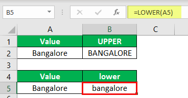
#9 Convert All Characters to UPPERCASE Values
If we want to convert all the text values to UPPERCASE, we can use the UPPER formula in excelUppercase function in Excel is used to convert lowercase text to uppercase.read more.
And if we want to convert all the text values to LOWERCASE values, then use the LOWER formula.
#10 Find Maximum and Minimum Values
If we want to find maximum and minimum values, we may use MAX and MIN functions in excelIn Excel, the MIN function is categorized as a statistical function. It finds and returns the minimum value from a given set of data/array.read more, respectively.
Things to Remember
- These are some of the important formulas/commands in excel which are used regularly.
- We can also use these functions at the advanced level.
- There are more advanced formulas in Excel which come under advanced level courses.
- Space is considered one character.
Recommended Articles
This article is a guide to Excel Commands. Here, we discuss the top 10 commands in Excel, examples, and a downloadable template. You may learn more about Excel from the following articles: –
- Break-Even Point in Excel
- Basic Excel Formulas List
- Create Custom Functions in Excel
- Write Formula in Excel
Below is a brief overview of about 100 important Excel functions you should know, with links to detailed examples. We also have a large list of example formulas, a more complete list of Excel functions, and video training. If you are new to Excel formulas, see this introduction.
Note: Excel now includes Dynamic Array formulas, which offer important new functions.
Date and Time Functions
Excel provides many functions to work with dates and times.
NOW and TODAY
You can get the current date with the TODAY function and the current date and time with the NOW Function. Technically, the NOW function returns the current date and time, but you can format as time only, as seen below:

TODAY() // returns current date
NOW() // returns current time
Note: these are volatile functions and will recalculate with every worksheet change. If you want a static value, use date and time shortcuts.
DAY, MONTH, YEAR, and DATE
You can use the DAY, MONTH, and YEAR functions to disassemble any date into its raw components, and the DATE function to put things back together again.

=DAY("14-Nov-2018") // returns 14
=MONTH("14-Nov-2018") // returns 11
=YEAR("14-Nov-2018") // returns 2018
=DATE(2018,11,14) // returns 14-Nov-2018
HOUR, MINUTE, SECOND, and TIME
Excel provides a set of parallel functions for times. You can use the HOUR, MINUTE, and SECOND functions to extract pieces of a time, and you can assemble a TIME from individual components with the TIME function.

=HOUR("10:30") // returns 10
=MINUTE("10:30") // returns 30
=SECOND("10:30") // returns 0
=TIME(10,30,0) // returns 10:30
DATEDIF and YEARFRAC
You can use the DATEDIF function to get time between dates in years, months, or days. DATEDIF can also be configured to get total time in «normalized» denominations, i.e. «2 years and 6 months and 27 days».

Use YEARFRAC to get fractional years:

=YEARFRAC("14-Nov-2018","10-Jun-2021") // returns 2.57
EDATE and EOMONTH
A common task with dates is to shift a date forward (or backward) by a given number of months. You can use the EDATE and EOMONTH functions for this. EDATE moves by month and retains the day. EOMONTH works the same way, but always returns the last day of the month.

EDATE(date,6) // 6 months forward
EOMONTH(date,6) // 6 months forward (end of month)
WORKDAY and NETWORKDAYS
To figure out a date n working days in the future, you can use the WORKDAY function. To calculate the number of workdays between two dates, you can use NETWORKDAYS.

WORKDAY(start,n,holidays) // date n workdays in future
Video: How to calculate due dates with WORKDAY

NETWORKDAYS(start,end,holidays) // number of workdays between dates
Note: Both functions automatically skip weekends (Saturday and Sunday) and will also skip holidays, if provided. If you need more flexibility on what days are considered weekends, see the WORKDAY.INTL function and NETWORKDAYS.INTL function.
WEEKDAY and WEEKNUM
To figure out the day of week from a date, Excel provides the WEEKDAY function. WEEKDAY returns a number between 1-7 that indicates Sunday, Monday, Tuesday, etc. Use the WEEKNUM function to get the week number in a given year.

=WEEKDAY(date) // returns a number 1-7
=WEEKNUM(date) // returns week number in year
Engineering
CONVERT
Most Engineering functions are pretty technical…you’ll find a lot of functions for complex numbers in this section. However, the CONVERT function is quite useful for everyday unit conversions. You can use CONVERT to change units for distance, weight, temperature, and much more.

=CONVERT(72,"F","C") // returns 22.2
Information Functions
ISBLANK, ISERROR, ISNUMBER, and ISFORMULA
Excel provides many functions for checking the value in a cell, including ISNUMBER, ISTEXT, ISLOGICAL, ISBLANK, ISERROR, and ISFORMULA These functions are sometimes called the «IS» functions, and they all return TRUE or FALSE based on a cell’s contents.

Excel also has ISODD and ISEVEN functions that will test a number to see if it’s even or odd.
By the way, the green fill in the screenshot above is applied automatically with a conditional formatting formula.
Logical Functions
Excel’s logical functions are a key building block of many advanced formulas. Logical functions return the boolean values TRUE or FALSE. If you need a primer on logical formulas, this video goes through many examples.
AND, OR and NOT
The core of Excel’s logical functions are the AND function, the OR function, and the NOT function. In the screen below, each of these function is used to run a simple test on the values in column B:

=AND(B5>3,B5<9)
=OR(B5=3,B5=9)
=NOT(B5=2)
- Video: How to build logical formulas
- Guide: 50 examples of formula criteria
IFERROR and IFNA
The IFERROR function and IFNA function can be used as a simple way to trap and handle errors. In the screen below, VLOOKUP is used to retrieve cost from a menu item. Column F contains just a VLOOKUP function, with no error handling. Column G shows how to use IFNA with VLOOKUP to display a custom message when an unrecognized item is entered.

=VLOOKUP(E5,menu,2,0) // no error trapping
=IFNA(VLOOKUP(E5,menu,2,0),"Not found") // catch errors
Whereas IFNA only catches an #N/A error, the IFERROR function will catch any formula error.
IF and IFS functions
The IF function is one of the most used functions in Excel. In the screen below, IF checks test scores and assigns «pass» or «fail»:

Multiple IF functions can be nested together to perform more complex logical tests.
New in Excel 2019 and Excel 365, the IFS function can run multiple logical tests without nesting IFs.

=IFS(C5<60,"F",C5<70,"D",C5<80,"C",C5<90,"B",C5>=90,"A")
Lookup and Reference Functions
VLOOKUP and HLOOKUP
Excel offers a number of functions to lookup and retrieve data. Most famous of all is VLOOKUP:

=VLOOKUP(C5,$F$5:$G$7,2,TRUE)
More: 23 things to know about VLOOKUP.
HLOOKUP works like VLOOKUP, but expects data arranged horizontally:

=HLOOKUP(C5,$G$4:$I$5,2,TRUE)
INDEX and MATCH
For more complicated lookups, INDEX and MATCH offers more flexibility and power:

=INDEX(C5:E12,MATCH(H4,B5:B12,0),MATCH(H5,C4:E4,0))
Both the INDEX function and the MATCH function are powerhouse functions that turn up in all kinds of formulas.
More: How to use INDEX and MATCH
LOOKUP
The LOOKUP function has default behaviors that make it useful when solving certain problems. LOOKUP assumes values are sorted in ascending order and always performs an approximate match. When LOOKUP can’t find a match, it will match the next smallest value. In the example below we are using LOOKUP to find the last entry in a column:

ROW and COLUMN
You can use the ROW function and COLUMN function to find row and column numbers on a worksheet. Notice both ROW and COLUMN return values for the current cell if no reference is supplied:

The row function also shows up often in advanced formulas that process data with relative row numbers.
ROWS and COLUMNS
The ROWS function and COLUMNS function provide a count of rows in a reference. In the screen below, we are counting rows and columns in an Excel Table named «Table1».

Note ROWS returns a count of data rows in a table, excluding the header row. By the way, here are 23 things to know about Excel Tables.
HYPERLINK
You can use the HYPERLINK function to construct a link with a formula. Note HYPERLINK lets you build both external links and internal links:

=HYPERLINK(C5,B5)
GETPIVOTDATA
The GETPIVOTDATA function is useful for retrieving information from existing pivot tables.

=GETPIVOTDATA("Sales",$B$4,"Region",I6,"Product",I7)
CHOOSE
The CHOOSE function is handy any time you need to make a choice based on a number:

=CHOOSE(2,"red","blue","green") // returns "blue"
Video: How to use the CHOOSE function
TRANSPOSE
The TRANSPOSE function gives you an easy way to transpose vertical data to horizontal, and vice versa.

{=TRANSPOSE(B4:C9)}
Note: TRANSPOSE is a formula and is, therefore, dynamic. If you just need to do a one-time transpose operation, use Paste Special instead.
OFFSET
The OFFSET function is useful for all kinds of dynamic ranges. From a starting location, it lets you specify row and column offsets, and also the final row and column size. The result is a range that can respond dynamically to changing conditions and inputs. You can feed this range to other functions, as in the screen below, where OFFSET builds a range that is fed to the SUM function:

=SUM(OFFSET(B4,1,I4,4,1)) // sum of Q3
INDIRECT
The INDIRECT function allows you to build references as text. This concept is a bit tricky to understand at first, but it can be useful in many situations. Below, we are using INDIRECT to get values from cell A1 in 5 different worksheets. Each reference is dynamic. If a sheet name changes, the reference will update.

=INDIRECT(B5&"!A1") // =Sheet1!A1
The INDIRECT function is also used to «lock» references so they won’t change, when rows or columns are added or deleted. For more details, see linked examples at the bottom of the INDIRECT function page.
Caution: both OFFSET and INDIRECT are volatile functions and can slow down large or complicated spreadsheets.
STATISTICAL Functions
COUNT and COUNTA
You can count numbers with the COUNT function and non-empty cells with COUNTA. You can count blank cells with COUNTBLANK, but in the screen below we are counting blank cells with COUNTIF, which is more generally useful.

=COUNT(B5:F5) // count numbers
=COUNTA(B5:F5) // count numbers and text
=COUNTIF(B5:F5,"") // count blanks
COUNTIF and COUNTIFS
For conditional counts, the COUNTIF function can apply one criteria. The COUNTIFS function can apply multiple criteria at the same time:

=COUNTIF(C5:C12,"red") // count red
=COUNTIF(F5:F12,">50") // count total > 50
=COUNTIFS(C5:C12,"red",D5:D12,"TX") // red and tx
=COUNTIFS(C5:C12,"blue",F5:F12,">50") // blue > 50
Video: How to use the COUNTIF function
SUM, SUMIF, SUMIFS
To sum everything, use the SUM function. To sum conditionally, use SUMIF or SUMIFS. Following the same pattern as the counting functions, the SUMIF function can apply only one criteria while the SUMIFS function can apply multiple criteria.

=SUM(F5:F12) // everything
=SUMIF(C5:C12,"red",F5:F12) // red only
=SUMIF(F5:F12,">50") // over 50
=SUMIFS(F5:F12,C5:C12,"red",D5:D12,"tx") // red & tx
=SUMIFS(F5:F12,C5:C12,"blue",F5:F12,">50") // blue & >50
Video: How to use the SUMIF function
AVERAGE, AVERAGEIF, and AVERAGEIFS
Following the same pattern, you can calculate an average with AVERAGE, AVERAGEIF, and AVERAGEIFS.

=AVERAGE(F5:F12) // all
=AVERAGEIF(C5:C12,"red",F5:F12) // red only
=AVERAGEIFS(F5:F12,C5:C12,"red",D5:D12,"tx") // red and tx
MIN, MAX, LARGE, SMALL
You can find largest and smallest values with MAX and MIN, and nth largest and smallest values with LARGE and SMALL. In the screen below, data is the named range C5:C13, used in all formulas.

=MAX(data) // largest
=MIN(data) // smallest
=LARGE(data,1) // 1st largest
=LARGE(data,2) // 2nd largest
=LARGE(data,3) // 3rd largest
=SMALL(data,1) // 1st smallest
=SMALL(data,2) // 2nd smallest
=SMALL(data,3) // 3rd smallest
Video: How to find the nth smallest or largest value
MINIFS, MAXIFS
The MINIFS and MAXIFS. These functions let you find minimum and maximum values with conditions:

=MAXIFS(D5:D15,C5:C15,"female") // highest female
=MAXIFS(D5:D15,C5:C15,"male") // highest male
=MINIFS(D5:D15,C5:C15,"female") // lowest female
=MINIFS(D5:D15,C5:C15,"male") // lowest male
Note: MINIFS and MAXIFS are new in Excel via Office 365 and Excel 2019.
MODE
The MODE function returns the most commonly occurring number in a range:

=MODE(B5:G5) // returns 1
RANK
To rank values largest to smallest, or smallest to largest, use the RANK function:

Video: How to rank values with the RANK function
MATH Functions
ABS
To change negative values to positive use the ABS function.

=ABS(-134.50) // returns 134.50
RAND and RANDBETWEEN
Both the RAND function and RANDBETWEEN function can generate random numbers on the fly. RAND creates long decimal numbers between zero and 1. RANDBETWEEN generates random integers between two given numbers.

=RAND() // between zero and 1
=RANDBETWEEN(1,100) // between 1 and 100
ROUND, ROUNDUP, ROUNDDOWN, INT
To round values up or down, use the ROUND function. To force rounding up to a given number of digits, use ROUNDUP. To force rounding down, use ROUNDDOWN. To discard the decimal part of a number altogether, use the INT function.

=ROUND(11.777,1) // returns 11.8
=ROUNDUP(11.777) // returns 11.8
=ROUNDDOWN(11.777,1) // returns 11.7
=INT(11.777) // returns 11
MROUND, CEILING, FLOOR
To round values to the nearest multiple use the MROUND function. The FLOOR function and CEILING function also round to a given multiple. FLOOR forces rounding down, and CEILING forces rounding up.

=MROUND(13.85,.25) // returns 13.75
=CEILING(13.85,.25) // returns 14
=FLOOR(13.85,.25) // returns 13.75
MOD
The MOD function returns the remainder after division. This sounds boring and geeky, but MOD turns up in all kinds of formulas, especially formulas that need to do something «every nth time». In the screen below, you can see how MOD returns zero every third number when the divisor is 3:

SUMPRODUCT
The SUMPRODUCT function is a powerful and versatile tool when dealing with all kinds of data. You can use SUMPRODUCT to easily count and sum based on criteria, and you can use it in elegant ways that just don’t work with COUNTIFS and SUMIFS. In the screen below, we are using SUMPRODUCT to count and sum orders in March. See the SUMPRODUCT page for details and links to many examples.

=SUMPRODUCT(--(MONTH(B5:B12)=3)) // count March
=SUMPRODUCT(--(MONTH(B5:B12)=3),C5:C12) // sum March
SUBTOTAL
The SUBTOTAL function is an «aggregate function» that can perform a number of operations on a set of data. All told, SUBTOTAL can perform 11 operations, including SUM, AVERAGE, COUNT, MAX, MIN, etc. (see this page for the full list). The key feature of SUBTOTAL is that it will ignore rows that have been «filtered out» of an Excel Table, and, optionally, rows that have been manually hidden. In the screen below, SUBTOTAL is used to count and sum only the 7 visible rows in the table:

=SUBTOTAL(3,B5:B14) // returns 7
=SUBTOTAL(9,F5:F14) // returns 9.54
AGGREGATE
Like SUBTOTAL, the AGGREGATE function can also run a number of aggregate operations on a set of data and can optionally ignore hidden rows. The key differences are that AGGREGATE can run more operations (19 total) and can also ignore errors.
In the screen below, AGGREGATE is used to perform MIN, MAX, LARGE and SMALL operations while ignoring errors. Normally, the error in cell B9 would prevent these functions from returning a result. See this page for a full list of operations AGGREGATE can perform.

=AGGREGATE(4,6,values) // MAX ignore errors, returns 100
=AGGREGATE(5,6,values) // MIN ignore errors, returns 75
TEXT Functions
LEFT, RIGHT, MID
To extract characters from the left, right, or middle of text, use LEFT, RIGHT, and MID functions:

=LEFT("ABC-1234-RED",3) // returns "ABC"
=MID("ABC-1234-RED",5,4) // returns "1234"
=RIGHT("ABC-1234-RED",3) // returns "RED"
LEN
The LEN function will return the length of a text string. LEN shows up in a lot of formulas that count words or characters.

FIND, SEARCH
To look for specific text in a cell, use the FIND function or SEARCH function. These functions return the numeric position of matching text, but SEARCH allows wildcards and FIND is case-sensitive. Both functions will throw an error when text is not found, so wrap in the ISNUMBER function to return TRUE or FALSE (example here).

=FIND("Better the devil you know","devil") // returns 12
=SEARCH("This is not my beautiful wife","bea*") // returns 12
REPLACE, SUBSTITUTE
To replace text by position, use the REPLACE function. To replace text by matching, use the SUBSTITUTE function. In the first example, REPLACE removes the two asterisks (**) by replacing the first two characters with an empty string («»). In the second example, SUBSTITUTE removes all hash characters (#) by replacing «#» with «».

=REPLACE("**Red",1,2,"") // returns "Red"
=SUBSTITUTE("##Red##","#","") // returns "Red"
CODE, CHAR
To figure out the numeric code for a character, use the CODE function. To translate the numeric code back to a character, use the CHAR function. In the example below, CODE translates each character in column B to its corresponding code. In column F, CHAR translates the code back to a character.

=CODE("a") // returns 97
=CHAR(97) // returns "a"
Video: How to use the CODE and CHAR functions
TRIM, CLEAN
To get rid of extra space in text, use the TRIM function. To remove line breaks and other non-printing characters, use CLEAN.

=TRIM(A1) // remove extra space
=CLEAN(A1) // remove line breaks
Video: How to clean text with TRIM and CLEAN
CONCAT, TEXTJOIN, CONCATENATE
New in Excel via Office 365 are CONCAT and TEXTJOIN. The CONCAT function lets you concatenate (join) multiple values, including a range of values without a delimiter. The TEXTJOIN function does the same thing, but allows you to specify a delimiter and can also ignore empty values.

=TEXTJOIN(",",TRUE,B4:H4) // returns "red,blue,green,pink,black"
=CONCAT(B7:H7) // returns "8675309"
Excel also provides the CONCATENATE function, but it doesn’t offer special features. I wouldn’t bother with it and would instead concatenate directly with the ampersand (&) character in a formula.
EXACT
The EXACT function allows you to compare two text strings in a case-sensitive manner.

UPPER, LOWER, PROPER
To change the case of text, use the UPPER, LOWER, and PROPER function

=UPPER("Sue BROWN") // returns "SUE BROWN"
=LOWER("Sue BROWN") // returns "sue brown"
=PROPER("Sue BROWN") // returns "Sue Brown"
Video: How to change case with formulas
TEXT
Last but definitely not least is the TEXT function. The text function lets you apply number formatting to numbers (including dates, times, etc.) as text. This is especially useful when you need to embed a formatted number in a message, like «Sale ends on [date]».

=TEXT(B5,"$#,##0.00")
=TEXT(B6,"000000")
="Save "&TEXT(B7,"0%")
="Sale ends "&TEXT(B8,"mmm d")
More: Detailed examples of custom number formatting.
Dynamic Array functions
Dynamic arrays are new in Excel 365, and are a major upgrade to Excel’s formula engine. As part of the dynamic array update, Excel includes new functions which directly leverage dynamic arrays to solve problems that are traditionally hard to solve with conventional formulas. If you are using Excel 365, make sure you are aware of these new functions:
| Function | Purpose |
|---|---|
| FILTER | Filter data and return matching records |
| RANDARRAY | Generate array of random numbers |
| SEQUENCE | Generate array of sequential numbers |
| SORT | Sort range by column |
| SORTBY | Sort range by another range or array |
| UNIQUE | Extract unique values from a list or range |
| XLOOKUP | Modern replacement for VLOOKUP |
| XMATCH | Modern replacement for the MATCH function |
Video: New dynamic array functions in Excel (about 3 minutes).
Quick navigation
ABS, AGGREGATE, AND, AVERAGE, AVERAGEIF, AVERAGEIFS, CEILING, CHAR, CHOOSE, CLEAN, CODE, COLUMN, COLUMNS, CONCAT, CONCATENATE, CONVERT, COUNT, COUNTA, COUNTBLANK, COUNTIF, COUNTIFS, DATE, DATEDIF, DAY, EDATE, EOMONTH, EXACT, FIND, FLOOR, GETPIVOTDATA, HLOOKUP, HOUR, HYPERLINK, IF, IFERROR, IFNA, IFS, INDEX, INDIRECT, INT, ISBLANK, ISERROR, ISEVEN, ISFORMULA, ISLOGICAL, ISNUMBER, ISODD, ISTEXT, LARGE, LEFT, LEN, LOOKUP, LOWER, MATCH, MAX, MAXIFS, MID, MIN, MINIFS, MINUTE, MOD, MODE, MONTH, MROUND, NETWORKDAYS, NOT, NOW, OFFSET, OR, PROPER, RAND, RANDBETWEEN, RANK, REPLACE, RIGHT, ROUND, ROUNDDOWN, ROUNDUP, ROW, ROWS, SEARCH, SECOND, SMALL, SUBSTITUTE, SUBTOTAL, SUM, SUMIF, SUMIFS, SUMPRODUCT, TEXT, TEXTJOIN, TIME, TODAY, TRANSPOSE, TRIM, UPPER, VLOOKUP, WEEKDAY, WEEKNUM, WORKDAY, YEAR, YEARFRAC
The complete Excel Functions list includes lookup, logic, date and time, text, information, and math functions with examples. Excel Functions are built-in presets, so Excel functions are hard-coded formulas with short, user-friendly names.
The list contains 300+ built-in Excel functions. Furthermore, look at the library of useful advanced functions (UDFs). If you want to jump to a specific category, use the list below; else, use the Search box for the latest tutorials.
- User-defined functions (must-have)
- Logical
- Text
- Lookup
- Date and Time
- Dynamic array
- Information
- Math
- Statistical
- Financial
Excel Function List
Logical
The functions below use logical tests and logical operators to evaluate a formula. Learn more about Boolean expressions.
LOOKUP
Here is the list of lookup functions in Excel. Of course, we already know that XLOOKUP changes everything. But it is worth keeping in mind the older lookup functions too.
User-defined functions
UDFs are advanced functions.
Date and Time
Date and Time functions help you create calculations based on dates and times.
Text
Text functions in Excel enable you to perform various calculations using strings.
Dynamic Array
Dynamic Arrays are resizable arrays. From now, Excel calculates the array automatically and returns values into multiple cells based on a formula entered in a single cell.
Information
Take a quick overview of information functions in Excel.
Math
Math Functions are great.
Math – Part 2
Financial
Use financial functions if you want.
Financial – Part 2
Statistical
Statistical – Part 2
Trigonometry
Engineering
Database
How to use Excel Functions?
To use a function, type an equal sign (=) in the formula bar or the cell to enter a function you want to use. After that, enter the function’s name and the arguments. There are custom functions in Excel, user-defined functions. If you want to learn more about how to solve complex tasks using UDFs, read our guide.
15 Most Common Excel Functions You Must Know + How to Use Them
Microsoft Excel is one of the most well-known computer applications. It has changed the way people and companies work with data.
Thus, learning Excel can help with both your career and your personal needs.
Excel runs using functions and there are roughly 500 of them! These range from basic arithmetic to complex statistics.

If you’re a new Excel user, this sheer quantity can be quite daunting.
So we are here to help you! 🤝
We have rounded up 15 of the most common and useful Excel functions that you need to learn. We also prepared a practice workbook for you to follow along with the examples. Download it here.
Let’s get started!
What are Excel functions?
Excel is used to calculate and manipulate numbers and text. To do this, you use formulas!
Formulas are expressions that tell Excel what you want to do with the data. They begin with the equal symbol (=) followed by a combination of operators and functions.
What are operators?
These are symbols that specify the type of calculation you want to perform on the elements of a formula.
For example, to add two numbers, you can type “=1+1” into a cell. Once you hit Enter, Excel will run the formula and return the result which is 2.
Here are some examples of common operators:

Excel automatically treats cell contents that start with (=) as formulas. This also applies when you begin a cell with the plus (+) or minus (-) symbols.
You can bypass this by adding a leading apostrophe (‘). This is how you can show formulas as text like in the table above.
Order of operation and using parentheses in Excel formulas
Generally, Excel follows PEMDAS when calculating formulas. PEMDAS means parentheses first, then exponents, then multiplication and division, then addition and subtraction.

What are functions?
These are predefined processes in Excel. Each function in Excel has a unique name and specific input(s). The function takes these inputs and performs the corresponding calculation.
The inputs or arguments of an Excel function are always enclosed in parentheses.
For example, this is the syntax for the MAX function:
=MAX(number1, [number2], …)
The list of numbers where you want to find the maximum value is placed inside the parentheses.

Using a cell or a range as input
As you learn more about Excel, you’ll find that Excel formulas rarely consist of individual numbers only like in the formula “=1+1”.

Thus, referencing cells is important in Excel and you can learn more by clicking here.
Alright! You’ve just learned how a function in Excel works.
Let’s dive right into the list! 🤿
We will start with basic Excel functions and then move on to more advanced functions.
Basic Math Functions (Beginner Level ★☆☆)
1. SUM
This is the first function in Excel that most new users need. As the name implies, the SUM function adds up all the values in a specified group of cells or range.
Syntax: =SUM(number1, [number2], …)
Try it out in the practice workbook.

If you want to get the total quiz score for each student, you can use the SUM function. In this case, the input range will be all four quiz scores for each student.
1. Type this formula into cell F2:
=SUM(B2:E2)
You can also type “=SUM(B2,C2,D2,E2)” but “=SUM(B2:E2)” is much simpler.

2. Press Enter. Excel then evaluates the formula and the cell returns the number for the total which is 360.
3. Copy this for the rest of the students or drag down the fill handle.

Notice that the SUM function ignores the cells containing text. (“X” meaning the student was unable to take the quiz)
Most of the basic math functions in Excel ignore non-numeric values such as text, date, and time.
2. COUNT
Next up is the COUNT function. It returns the number of cells containing numeric values within the input range.
Syntax: =COUNT(value1, [value2], …)
1. To get the number of quizzes taken by each student, use this formula in cell G2:
=COUNT(B2:E2)
2. Hit Enter and fill in the rows below.

If you would like to include non-numeric values in the count, you can use the COUNTA function. To count the number of blank cells, you can use the COUNTBLANK function.
Learn more about the COUNT function and its variants here.
3. AVERAGE
The average of a list of numbers is just the total divided by how many numbers there are in that list.
This is easy enough to calculate the quiz scores. You already have the SUM and the COUNT of quizzes for each student.
But, it gets even easier using the AVERAGE function in Excel.
Syntax: =AVERAGE (value1, [value2], …)
1. Type this into cell H2:
=AVERAGE(B2:E2)
2. Hit Enter and fill in the rows below.


Logical Functions (Intermediate Level – ★★☆)
Let’s raise the difficulty level a little bit.
A logical function in Excel allows you to make comparisons and use the results to change how a formula calculates.
4. IF
The IF function is a very popular function in Excel and it is actually quite easy to learn.
Syntax: =IF(logical_test, value_if_true, [value_if_false])
This function checks if a logical test is either TRUE or FALSE. It then returns the specified value based on the result.

Using the average score of each student, try to assign PASS or FAIL grades. Assume that the passing score for this class is 60.
1. Begin the formula in cell C2 with “=IF(“
The logical_test is to check if the average score in Column B is greater than or equal to (>=) the passing score of 60.
2. So, the formula becomes:
=IF(B2>=60,
If the comparison returns TRUE, then the formula should return the text “PASS”. Thus, the value_if_true argument should be “PASS”.
And if it returns FALSE, then the value_if_false argument should be “FAIL”.
3. Thus, the formula becomes:
=IF(B2>=60,”PASS”,”FAIL”)
4. Hit Enter and fill in the rows below.

What if you needed to assign grades according to a scale instead of just “PASS” and “FAIL”?
For that, you have to use multiple criteria or logical tests. While this is possible using nested IF functions, it can get messy very quickly. Instead, you can use the IFS function.
5. IFS function
The IFS function was introduced in Excel 2016 to replace nested IF functions.
This function works by evaluating the first logical test or criteria. It returns the corresponding value if it is TRUE. But if it is FALSE, the function proceeds to evaluate the second criteria, and so on.
📖 In other words, the IFS function outputs the value that corresponds to the first specified criteria that is true.
Syntax: =IFS(logical_test1, value_if_true1, [logical_test2], [value_if_true2],..)

1. First, the formula should check if the average score (column B) is above or equal to 90. If yes, it should return “A”.
=IFS(B2>=90,”A”,
2. If not, it should then check if the average score is greater than or equal to 80. If yes, it should return “B”. If you do this up to grade D, the formula becomes:
=IFS(B2>=90,”A”,B2>=80,”B”,B2>=70,”C”,B2>=60,”D”,
3. For the last grade “F”, put “TRUE” for the logical test.
The IFS function will only evaluate the last specified criteria if all of the previous logical values were FALSE. Thus, you can set the last criteria to always be TRUE thus making it a “catch all” statement.
The final formula is then:
=IFS(B2>=90,”A”,B2>=80,”B”,B2>=70,”C”,B2>=60,”D”,TRUE,”F”)

PRO-TIP:
You can use absolute cell references and a reference table when working with long formulas.
That way, you don’t have to revisit all of the arguments in the formula if you need to change some values.
For example, using the table and formula shown below, you can easily change the grading scale in use.
=IFS(B2>=$H$2,$F$2,B2>=$H$3,$F$3,B2>
=$H$4,$F$4,B2>=$H$5,$F$5,TRUE,$F$6)

Text Functions (Intermediate Level – ★★☆)
In this next section, you will see how Excel can also be used to manipulate text.
In the “Class List” worksheet of the practice workbook, the full name of each student is listed in Column A. Your goal is to rearrange these from “first name last name” to “last name_first name” in Column F.

To do this, you first have to extract the first name and the last name from Column A.
6. FIND
The names are separated by a space character ” “. So, you have to identify the position of the space within each text string in Column A.
The FIND function in Excel returns the number or position of a specified character or substring within another text string.
Syntax: =FIND(find_text, within_text, [start_num])
To get the position of the space ” “, type this formula:
=FIND(” “,A2)

Next, take a look at the LEN function.
7. LEN
This function returns the number of characters in a text string.
Syntax: =LEN(text)
To get the number of characters in each student’s name:
=LEN(A2)

Now you can move on to extracting the first and last name using the MID function in Excel.
8. MID
This function extracts a given number of characters from the middle of a text string.
Syntax: = MID(text, start_num, num_chars)
It is one of three text functions that are used to extract text. The other two are LEFT and RIGHT which extract text from the start and end of a text string respectively.
The first name starts at the very first character of the text string. So, you extract starting from position 1. Then the length of the first name is given by the position of the space character minus 1.
So, the formula to extract the first name or first word from a text string is:
=MID(A2,1,B2-1)
Or, you can express it directly using the FIND formula earlier.
=MID(A2,1,FIND(” “,A2)-1)

For the last name, you can extract it starting from the position of the space character plus 1. Its length is just the length of the entire text string minus the position of the space character.
=MID(A2,B2+1,C2-B2)
Or, using the FIND and LEN formulas earlier:
=MID(A2,FIND(” “,A2)+1,LEN(A2)-FIND(” “,A2))

Now you can combine the last name and the first name in the desired order using the CONCAT function.
9. CONCAT
Like IFS, CONCAT is another newly introduced function in Excel 2016. It replaced the old CONCATENATE function.
Syntax: =CONCAT(text1, [text2],…)
Combine the last name and the first name with a comma and space character “, ” in between.
=CONCAT(E2,”, “,D2)

PRO-TIP:
In the above example, you used helper columns for FIND, LEN, and MID to help build the final formula and visualize how it works.
In real-world applications, you can use a single long formula to get the results like this:
=CONCAT(MID(A2,FIND(” “,A2)+1,LEN(A2)
-FIND(” “,A2)),”, “,MID(A2,1,FIND(” “,A2)-1))

Lookup and Reference Functions (Advanced Level – ★★★)
In this final section, we will focus on functions that allow you to look for specific data points and refer to them.
Take a look at the “Schedule” worksheet.

10. COLUMN
The COLUMN function in Excel returns the column number of a given cell.
Syntax: =COLUMN([reference])
Let’s try to assign specific dates for each quiz. For example, you may want the quizzes to be held every Monday. This means that the first quiz date should be offset by 1 week or 7 days for each succeeding quiz date.
You can use the column number to multiply the 7 days offset for each week like this:
=$B$2+(COLUMN()-2)*7

Two (2) is subtracted from the column number so that the sequence starts at 1.
You can also get this result using the much simpler “=B2+7” since you are only adding a fixed number of days to each date. 🤔
But, using the COLUMN function, you can create complex patterns.
Take this pattern for example:
The quizzes are still held every Monday. But every third week, they are held on Wednesday instead.
Here is the formula for this pattern:
=$B$2+(COLUMN()-2)*7+IF(MOD(COLUMN()-1,3)=0,2,0)


The MOD function in Excel returns the remainder after a number is divided by a given divisor. It’s part of the Math & Trig group of functions.
This group includes other fun functions such as ABS which returns the absolute value of a number and ROUND which rounds a number to a specified number of digits.
Learn more about the function groups towards the end of this article!
11. ROW
Next, take a look at the ROW function. It works exactly like COLUMN but it returns the row number instead.
Syntax: =ROW([reference])
In this next example, you will assign the seating plans. You can try different seating arrangements using the ROW function.
Assume R1C1 is the seat closest to the teacher’s desk.
1. You can have the students seated one seat after another and in two columns:
=CONCAT(“R”,MOD(ROW()-6,3)*2+1,”C”,INT((ROW()-6)/3)*2+1)

2. Or they can sit in rows of 3 and columns of 2
=CONCAT(“R”,MOD(ROW()-6,2)*2+1,”C”,INT((ROW()-6)/2)*2+1)

3. You can also sit them in the farthest rows:
=CONCAT(“R”,MOD(ROW()-6,2)*4+1,”C”,INT((ROW()-6)/2)*2+1)

4. Or in the farthest columns:
=CONCAT(“R”,MOD(ROW()-6,3)*2+1,”C”,INT((ROW()-6)/3)*4+1)

Manually creating seating patterns for small sets like this one is easy. But a formula like those shown above definitely helps especially for larger sets like 50, 100, or even more.
The COLUMN and ROW functions are rarely used on their own. Like IF and IFS, you use them with other functions to change how the formula is calculated.
12. MATCH
Now, open up the “Lookup” worksheet.
In the next few examples, you will create a search feature that allows students to look up their names. They can then see their scores from past quizzes and their assigned seats for the next quizzes.
To start, you will use the MATCH function. It searches for a specified item within a given range of cells. It then returns the relative position of the first match.
Syntax: =MATCH(lookup_value, lookup_array, [match_type])
- The lookup_value is the item you want to search for. So, set this to cell B2.
- The lookup_array is the range or table array where you want to search. Use F2:F7 from the “Class List” worksheet.
- For the match_type, set this to zero so that the function searches for an exact match. (Learn more about MATCH and the different match types in this article)
The formula then becomes:
=MATCH(B2,’Class List’!F2:F7,0)

However, it only works correctly if the name is entered exactly as it is written in Column F of the Class List.
To fix this, you can use the asterisk “*” wildcard character so that searching for either first or last name works.
You can also enclose the formula in an IFNA function. This way, if the formula cannot find the given name in the table, it will return a phrase like “No result found”.


13. INDEX
The INDEX function retrieves a value from a given table array based on the provided row and column numbers.
Syntax: =INDEX (array, row_num, [col_num])
Similar to the MATCH example, you need to specify where the range or array lookup is.

For row_num, you can use the earlier MATCH result at Cell B5. Then for col_num, use 1 for the First Name:
=INDEX(‘Class List’!D2:E7,B5,1)

And set col_num to 2 for the Last Name.
=INDEX(‘Class List’!D2:E7,B5,2)

Just like that, you have a working search 🔍 formula!
This is just a small example of the countless possibilities using the INDEX and MATCH combination. Click here for more examples!
14. VLOOKUP
The VLOOKUP function in Excel works similarly to the INDEX and MATCH combination. It is faster to set up but it is less versatile. VLOOKUP also only works if your lookup array is at the leftmost of the reference table.
Syntax: =VLOOKUP (lookup_value, table_array, col_index_num, [range_lookup])
This time, you will use the First Name result (cell B6) as the lookup_value. Use this and VLOOKUP to retrieve the given student’s scores from the “Quiz Scores” worksheet.
=VLOOKUP($B$6,’Quiz Scores’!$A$2:$E$7,COLUMN(),FALSE)

For the seat assignment, use the Last Name result followed by the asterisk wild character.
=VLOOKUP($B$7&”*”,Schedule!$A$6:$E$11,COLUMN(),FALSE)

15. INDIRECT
The last function that you will be learning about today is also one of the most powerful in Excel.
INDIRECT allows you to specify cell references using text strings.
SYNTAX: =INDIRECT(ref_text, [a1])
For example, instead of typing “=A1”, you can type “=INDIRECT(“A”&1). This means you can dynamically change references.
Let’s take the INDEX & MATCH formula you used to retrieve the Last Name. You can get the same result using this formula:
=INDIRECT(“‘Class List’!”&”E”&(B5+1))

The INDIRECT function opens up so many possibilities with dynamic references in Excel. I highly this article for an in-depth tutorial on INDIRECT.
That’s it – Now what?
As you have just learned, Excel offers so many different functions to choose from. Luckily, Excel has brought them all together in the Formulas tab.

You can look for an Excel function using search keywords or you can also select from the categorical dropdowns.
For example, click on the Financial group to find functions that can help you calculate items like net present value, future value, cumulative interest paid, cumulative principal paid, etc.

You can also click on More Functions which opens up even more possibilities for advanced Excel formulas.
For example, the Statistical group is useful if you need to calculate a statistical value. This includes functions for maximum value, minimum value, forecast value, gamma function value, etc. You can insert a cumulative distribution function and other useful tools for data analysis.

Learn how to use these formulas and more by signing up for my free online Excel course.
We will help you make the most out of your Excel experience! 📈
Other relevant resources
If you enjoyed this article, you can visit my YouTube channel for more in-depth tutorials and other fun stuff!
Did you know that the Flash Fill feature can help speed up your work by automatically filling a repetitive pattern Excel detects from your data? Learn more here.
Thanks for reading! 😄
Kasper Langmann2023-02-23T11:47:15+00:00
Page load link