Comma style in excel

Excel Comma Style (Table of Contents)

Comma Style in Excel
How to Apply Comma Style in Excel?

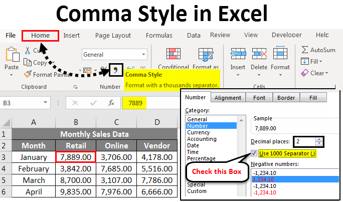
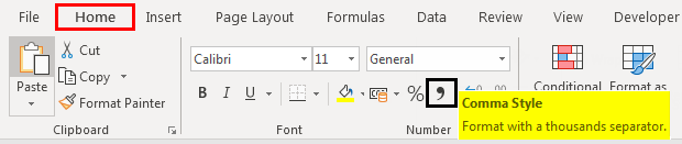
Comma style is Excel mainly used for numbers to distinguish the different lengths like hundreds, thousands, millions, etc. This allows users to read and spell the numbers incorrect form. To enable the comma in any cell, select Format Cells from the right-click menu and, from the Number section, check the box of Use 1000 separator (,). We can also use the Home menu ribbons’ Commas Style under the number section. We can also even use short cut keys by pressing ALT + H + K simultaneously to apply comma style.

Comma style format is categorized under the Number format section in the Home tab.

Comma style format is also referred to as thousands separator.

This format will be very helpful when you are working on a large table of financial sales data (Quarterly or half or Annual sales data), Comma style format is applied here, and numbers appear better. It is used to define the behavior of digits in relation to the thousands or lacks or millions or billions of digits. Comma Style format offers a good alternative to the Currency format. Comma style format inserts commas in larger numbers to separate thousands, hundred thousand, millions, billions, and so on.

Comma style is a type of number format where it adds commas to large numbers, adds two decimal places (i.e. 1000 becomes 1,000.00), displays negative values in closed parentheses & represents zeros with a dash (–).

The shortcut key for comma style is ALT + HK.

Prior to working on comma style number format, we need to check whether decimal & thousand separators are enabled or not in excel. If it is not enabled, we need to enable it & update it by the below-mentioned steps.

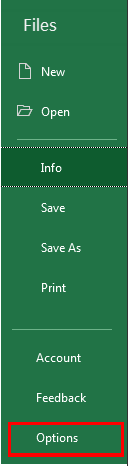
To check decimal and thousands of separators in Excel, click the File tab.

Click Options in the list of items on the left-hand side, Excel Options dialog box appears.

In the Excel Options dialog box. Click Advanced in the list of items on the left-hand side.
Under the editing options, Click or Tick on the Use system separators checkbox if there is no checkmark in the box. The Decimal separator and Thousands separator edit boxes displayed once you click on the “Use system separators” checkbox. Here I selected a comma as the thousands separator and a full point as the decimal separator. After that, click on OK.

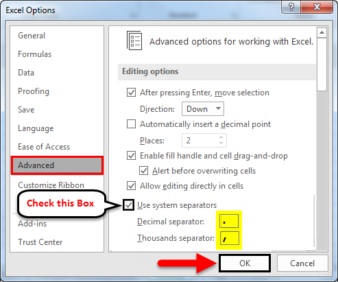
These separators are automatically inserted into all the numbers in your workbook when you use the comma style number format.

Different types of Numeric value or Number types that you come across in sales data are as follows.

Positive
Negative
Zero
Text

How to Apply Comma Style in Excel?

Let’s check out how comma style number format works on different types of Numeric value or Number types in Excel.

You can download this Comma Style Excel Template here – Comma Style Excel Template

Comma Style in Excel – Example # 1

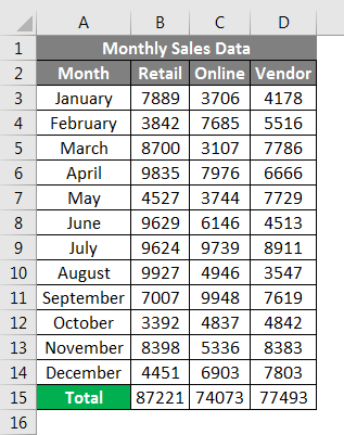
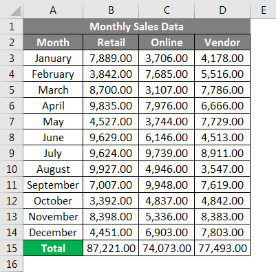
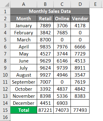
In the below-mentioned example, I have monthly sales data of a company, which contains retail, online & vendor sales numbers on a monthly basis; in this raw sales data, the appearance of the data is without any number format applied to it.

So, I need to apply the comma style number format for these positive sales values.

To display sales numbers with comma style format in Excel:

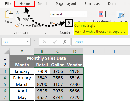
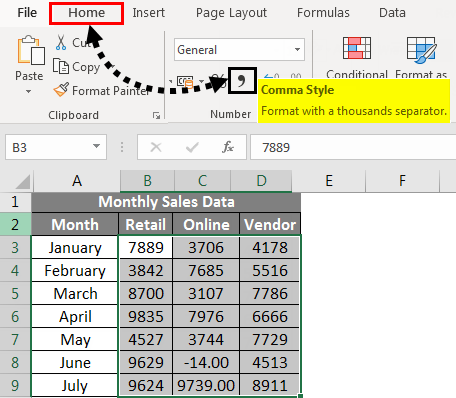
Select the cells containing numeric sales values for which I want to display numbers with comma style number format.
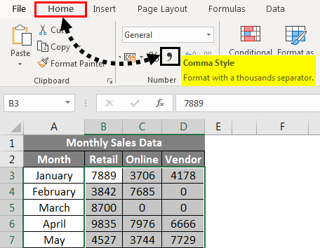
On the Home tab, you can select the Comma symbol & click on the Comma Style .command in the Number group.

; after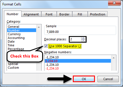

Once you have clicked on the Comma Style button, you can see the changes in the sales value, where excel separates the thousands with a comma and adds two decimal places at the end.

In the first cell, you can observe where 7889 becomes 7,889.00. The result is shown below.

Comma Style in Excel – Example # 2

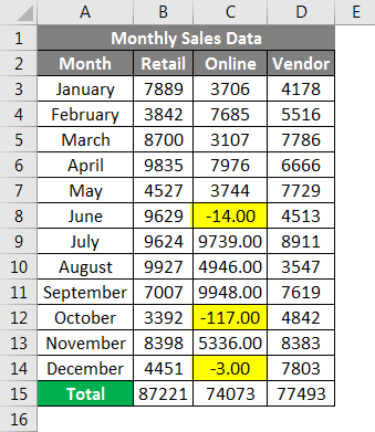
In the below-mentioned example, I have monthly sales data of a company, which contains retail, online & vendor sales numbers on a monthly basis, in this raw sales data, it contains both positive & negative values. Currently, the appearance of the sales data is without any number format applied to it.

So, I need to apply comma style number format for these positive & negative values.

To display numbers with comma style format in Excel:

Select the cells containing numeric sales values for which I want to display numbers with comma style number format. On the Home tab, you can select the comma symbol & click on the Comma Style command in the Number group.

Once you have clicked on the Comma Style button, you can see the changes in the sales value.

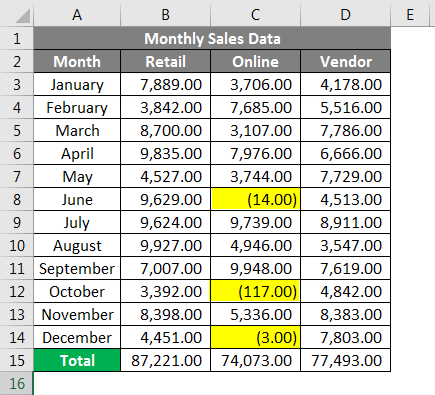
Where excel separates the thousands with a comma and adds two decimal places at the end, and it encloses negative sales values in a closed pair of parentheses.

Comma Style in Excel – Example # 3

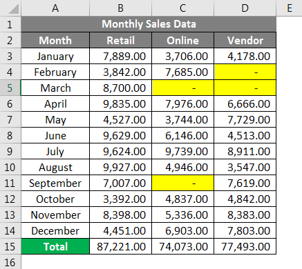
In the below-mentioned example, I have monthly sales data of a company, which contains retail, online & vendor sales numbers on a monthly basis, in this raw sales data, it contains both positive & Zero values. Currently, the appearance of the sales data is without any number format applied to it.

So, I need to apply a comma style number format for these positive & Zero values.

To display numbers with comma style format in Excel:

Select the cells containing numeric sales values for which I want to display numbers with comma style number format. On the Home tab, you can select the comma symbol & click on the Comma Style command in the Number group.

Once you have clicked on the Comma Style button, you can see the changes in the sales value.

Where excel separates the thousands with a comma and adds two decimal places at the end, and a dash symbol represents zero values.

Things to Remember

The comma style number Format option in excel makes your data easier to access & readable; it also helps you to set up your sales data at an industry standard.
Apart from various number format options in excel, you can create your own custom number format in Excel based on your choice.

Comma Style Formatting in Excel

The comma style is a formatting style used in visualizing numbers with commas when the values are over 1,000. Such as, if we use this style on data with a value of 100,000, then the result displayed will be as (100,000). This formatting style can be accessed from the “Home” tab in the number section and click on the 1,000 (,) separator, known as the comma style in Excel.

For example, we have a company’s monthly sales and production dataset without a number format. In such cases, if we need to apply the comma style number format for the positive values, comma style formatting in Excel separates the thousands with a comma. It adds two decimal places at the end and a dash symbol at the zero values. It can also help create the custom number format of our choice. Moreover, it also makes it easier to access and increases readability by setting up data at an industry standard.

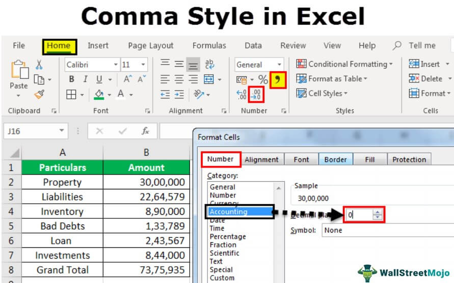
The comma style format (also known as the thousands separator) regularly goes with the “Accounting” format. Like the “Accounting” position, the comma arrangement embeds commas in bigger numbers to isolate thousands, hundred thousand, millions, and all values considered.

The standard comma style format contains up to two decimal points and a thousand separators and locks the dollar sign to the extreme left half of the cell. Negative numbers are shown in enclosures. To apply this format in a spreadsheet, we must feature every cell and click “Comma Style Format” under formatting choices in ExcelFormatting is a useful feature in Excel that allows you to change the appearance of the data in a worksheet. Formatting can be done in a variety of ways. For example, we can use the styles and format tab on the home tab to change the font of a cell or a table.read more.

Comma Style Formatting in Excel
- How to Apply Comma Style in Excel (accounting format)?
- Excel Shortcuts to Use Comma Style Format
- Advantages
- Disadvantages
- Things to Remember
- Recommended Articles

How to Apply Comma Style in Excel (accounting format)?

You can download this Comma Style Excel Template here – Comma Style Excel Template

Lets us start the below steps.

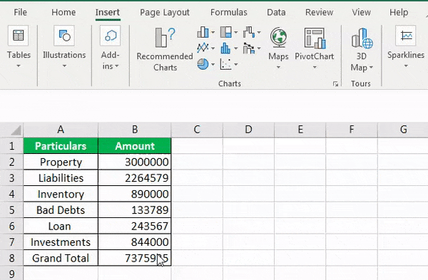
We must first enter the values in Excel to use the comma number format in Excel.
We can use accounting Excel format in the Number format ribbon, select the amount cell, click on ribbon home, and select the Comma Style from the Number format column.
Once we click on the Comma Style, it will provide the comma-separated format value.
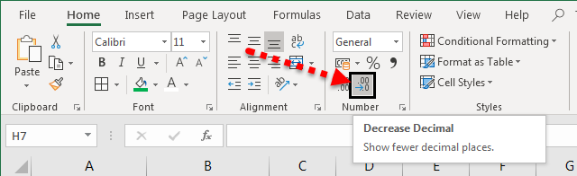
If we want to remove the decimal, we must click on the icon under Number on Decrease Decimal.
Once we remove the decimal, we can see below the value without decimals.
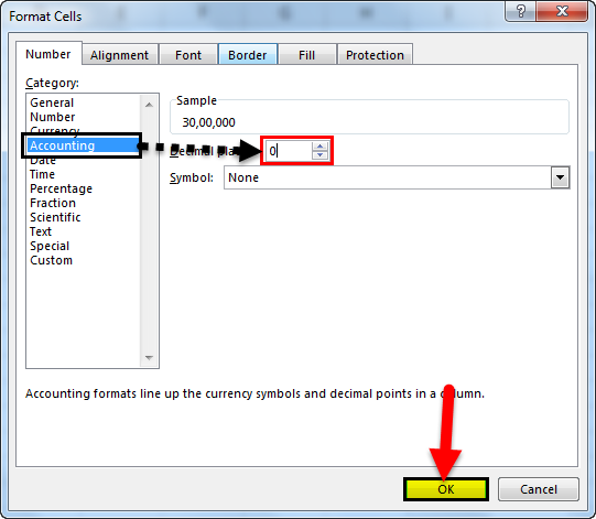
Then, we must select cells under the Amount column. Then, right-click on it, and choose Format Cells. After that, select the Accounting option under the Format Cells. If we do not want the decimal places, we can insert 0 under decimal places. And click on OK.
Below is the formatted data after removing decimal points.

Excel Shortcuts to Use Comma Style Format

We must select the cells which need to format.

Press the Alt key that enables the commands on the ExcelVLOOKUP function, IF condition, CONCATENATE function, find MAXIMUM and MINIMUM values are the most commonly used excel commands.read more ribbon.

Press H to select the Home tab in the Excel ribbonThe ribbon is an element of the UI (User Interface) which is seen as a strip that consists of buttons or tabs; it is available at the top of the excel sheet. This option was first introduced in the Microsoft Excel 2007.read more, it enables the Home tab of Excel.
Press 9 to decrease the decimal, and press 0 to increase the decimal point from values.
If you want to open the format cells dialogue, press Ctrl+1.
If you want to show a monetary valueMonetary value refers to the value of a product or service measured in terms of money. read more without a currency symbol, you can click None under option format cells.
Like the “Currency” format, the “Accounting” group is utilized for financial qualities. In any case, this arrangement adjusts the decimal purposes of numbers in a section. Likewise, the “Accounting” design shows zeros as dashes and negative numbers in brackets. Like the “Currency” format organizes, we can determine what number of decimal spots we need and whether to utilize a thousand separators. We cannot change the default show of negative numbers except if we make a custom number organization.

Advantages

It helps to format the number when we are dealing with currency.
It provides help in showing the correct value with commas.
It is just a one step process.
It is very easy and convenient to use.

Disadvantages

It always enables the number format with a thousand separators.
It provides the decimal points of two places while using this function.

Things to Remember

Rather than choosing a range of cells, we can likewise tap on the letter over a column to select the whole column or the number next to a column to select an entire row. We can likewise tap the little box to one side of “A” or above “1” to choose the whole spreadsheet at once.
We must always check and remove it if we do not need a comma.
Decimal is also the user’s choice if they want to put a decimal in values or not.
A custom Excel number format changes just the visual representation. For example, how value is shown in a cell. The basic value put away in a cell is not changed.
The comma Excel format is a default option to show numbers with a comma in the thousands place and includes two decimal places (Eg: “13000” becomes “13,000.00). It may also enable us to change the visible cell styles in an area of the ribbon to easily select different options for comma and display format as required in our sheet.

Apply Comma Style Using the Home tab

First, select the cells or range of cells or the entire column where to apply the comma style.
After that, go to the “Home” tab and click on the comma (,) icon under the “Number” group on the ribbon.
Once you click on the comma (,) icon, your selected range will get applied with comma separators in the number values.

To increase or remove the decimal values from the numbers, simply select the range and then click on the “Increase or Decrease decimal value” icon under the same “Number” group on the ribbon.

Apply Comma Style Using Format Cells Option

First, select the cells or range of cells or the entire column where to apply the comma style.
After that, right click on the mouse and select the “Format Cells” option from the drop-down list.
Once you click on “Format Cells” you will get the “Format Cells” dialog box opened.
Now, under the “Number” tab, select the “Number” option and then checkmark the “Use 1000 Separator” box.
In the end, Click OK, and your selected range will get applied with comma separators in the number values.
To remove the decimal values, enter zero (0) in the “Decimal places” field.

Change the Comma Style Separators from Lakhs to Million format

Sometimes, comma separators show numbers values separated in lakhs due to the default region and currency format of your system, but can change the currency format to millions format by following the below steps:

First, go to your system “Control Panel” and click on the “Change date, time, or number formats” link under the “Clock and Region” or “Region and Language” option. (Option names could be different depending on the Windows version)
After that, click on “Additional Settings” within the “Region” dialog box.
Once you click on “Additional Settings”, you will get the “Customize Format” dialog box opened.
Now, select the “Currency” header and then select the format to million style format of separator commas option in digit grouping.
In the end, click Apply and then Ok within the “Customize Format” dialog box and then in the “Region” dialog box.
Once you are done, close and open the Excel file again and apply comma style and you will get your selected range will get applied with comma separators in thousand, hundred thousand, and million to the number values.

Apply Comma Style Using Keyboard Shortcut

Select the entire column or the range where to apply comma style and then press the Alt+ H + K keys and you will get your selected range applied with comma separators.

Источник

The comma style is quite commonly used when people work with financial data in Excel.

It helps improve the readability of your data as it adds commas between digits (and also adds decimals).

In this tutorial, I will show you how to quickly apply the comma style in Excel using a couple of different methods (including a keyboard shortcut).

I will also show you how you can customize the format and increase or decrease the number of decimal places in the numbers.

Let’s have a look at a couple of ways to apply the comma style to your data in Microsoft Excel (including a keyboard shortcut).

Using the Ribbon in Excel

Below I have a data set where I have month names in column A and the sales figures in column B, and I want to show the sales figures data with a comma-style applied to the numbers.

Here are the steps to do this:

Click the Home tab
In the Number group, click on the ‘Comma Style’ icon (the big black comma icon)

That’s it!

The comma style format would be applied to the selected cells.

When you apply a comma-style format to cells that contain numbers, you notice a few things change:

The numbers are now separated by commas. The grouping of the numbers (i.e., numbers between the commas) depends on your regional settings. This can be changed and we’ll see how to do that later in this tutorial)
A decimal point is added and two digits are added after the decimal point

If you do not want the decimal numbers in your data set, you can remove these by clicking on the Home tab and then clicking on the Decrease Decimal icon (it’s right next to the Comma Style icon)

And in case you want to increase the number of digits after the decimal point, you can use the increase decimal icon

Keyboard Shortcut to Apply the Comma Style

If you would rather prefer to use a keyboard shortcut to apply the comma-style format to your data set, you can use the below keyboard shortcut:

ALT + H + K

You need to press these keys in succession, i.e., one after the other.

Using the Format Cells Dialog Box

Another method to apply comma formatting to your data set is by using the Format Cells dialog box.

While the previous method of using the ribbon or the keyboard shortcut is faster, with the Format Cells dialog box, you get a little more control over the formatting that you can apply.

Below are the steps to apply comma style to a data set using the Format Cells dialog box:

Select the cells on which you want to apply the comma-style format
Right-click on the selection
Click on Format Cells. This will open the Format Cells dialog box

In the Format cells dialog box, select the Number tab (if not selected already)

Select the number tab in Format cells dialog box

In the Category list, select Number
Check the ‘Use 1000 separator’ option

[Optional] Change the number of decimal places

One additional option that you get when you use the Format Cells dialog box is the ability to apply red color to cells with negative values.

You can choose any of the four options in the ‘Negative Numbers; box. This allows you to show negative values in red color with or without the minus sign.

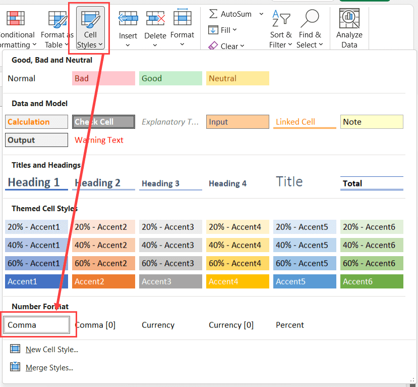
Using the Cells Styles Option

Another quick way to apply comma style in your data set is by using the styles option in Excel.

Below are the steps to use cell styles to apply comma style on your data set:

Select the cells that have the numbers on which you want to apply the comma style
Click the Home tab

In the Styles group, click on ‘Cell Styles’
From the options that show up, click on the ‘Comma’ option in ‘Number Format’

One benefit you can get from using the Cell Styles options is that you can create your own cell style that can be applied with a single click.

For example, if in addition to applying the comma style, you also want the cells to have a specific type of border or fill color or alignment/font, you can create a new style and specify all these formattings to it.

This can be done using the ‘New Style’ option that shows up when you click on the ‘Cell Styles’ option in the ‘Home’ tab.

Once you have created a new style, you can easily apply it to any cell by going to the Cell Styles options and clicking on that style (it would show up in the options once you create it)

Changing the Comma to Decimal in Numbers (or Vice Versa)

In many regions, there’s a difference in the way numbers are shown.

For example, in South America and some European countries, a decimal is used instead of a comma, and a comma is used instead of a decimal.

To give you an example, instead of 12,34,567.00, the format would be 12.34.567,00

While Excel is smart enough to take care of the formatting when you share your Excel file with someone who has the regional setting that uses decimal instead of a comma, let me still show you a method that will allow you to make this change on your system.

Below are the steps to change the comma to decimal in Excel:

Click the Home tab
Click on Options
In the Excel Options dialog box, select Advanced

In the ‘Editing’ options, uncheck ‘Use system separators’
Change the Decimal Separator to comma (,)
Change the Thousands separator to decimal point (.)

Click Ok

The above steps would turn off your system’s in-built setting, and use the separators that you have specified.

In this example, I have simply interchanged a decimal point and a comma, but you can also use other separators if you want.

Also note that this does not change the number in the back end, and only changes the way the numbers are being displayed to the user.

If you want to revert these changes and get the default setting back, open the Excel Options dialog box and check the ‘Use system separators’

How to Change Comma Style from Lakhs to Millions in Excel?

Different regions have different ways of comma styles that they apply to numbers.

For example, in the US and UK, a comma is placed after every third digit (when going from left to right). So, 1 million would be 1,000,000

On the other hand, another popular comma style method is using Lakhs and Crores, where a comma is placed after the first 3 digits (considering left to right), and then every second digit. So 1 million would be 10,00,000

If you have the lakh comma style and you want to change it into the million comma style, you can do that by using the steps below:

Go to the Control Panel in your system (you can search for it in the search bar)
Click on the ‘Change date, time, or number format’ option

In the Region dialog box that opens up, click on the Additional Settings button. This will open the Customize Format dialog box.

Click on the Currency tab

In the ‘Digit grouping’ dropdown, select the million comma style

Select the million comma format grouping

Click on Apply

Once the above changes are done, all the numbers would be displayed in the million, style format.

In case you want to revert to the original default settings, you can do that by clicking on the Reset button in the Currency tab in the Customize Format dialog box.

In this tutorial, I covered three different methods to apply the comma-style format for numbers in Excel (including a keyboard shortcut).

I also covered how to interchange a comma with a decimal point in numbers (which is the accepted format in many regions), as well as the process to change the Lakh comma style format to the million comma style format.

Other Excel tutorials you may also find useful:

How to Apply Short Date Format in Excel? 3 Easy Ways!
How to Apply Strikethrough in Excel (Shortcut)
How to Remove Commas in Excel (from Numbers or Text String)
How to Apply Accounting Number Format in Excel
How to Format Phone Numbers in Excel
How to AutoFormat Formulas in Excel (3 Easy Ways)
What does $ (dollar sign) mean in Excel Formulas?
How to Change Commas to Decimal Points in Excel?
Apply Currency Format in Excel (Shortcut)
How to Apply Long Date Format in Excel?

Источник

How to Apply Comma Style in Excel – Thousand Separator Format

Do you know the comma style and the thousand separator format are the same functions in Excel?

Also, do you know how to apply comma style in Excel?

Basically, the comma style in Excel lets you change the large number values while using commas added as separators. These separators are used to make a distinction between the number value lengths into thousands, hundred thousand, millions, and so on.

While using comma format, you will notice the decimal values of the numbers as well. You can find similarities between an accounting system format and the comma format.

How to Apply Comma Style in Excel? (Accounting Format)

To understand this method, you need to follow the steps given here:

First, add the values in Excel so that you can easily use the comma number format.

In the Number format ribbon, you can even use accounting Excel format as well. For this, choose the cells and click on the Home tab. Choose the Comma Style from the Number Format column.

As you click on the Comma Style, you will notice the comma-separated format value appears.

To delete the decimals, click on the icon given under the Number on Decrease Decimal.

Once the decimals are deleted, the value without decimals will appear.

Now, choose the cells given under the Amount column. Right-click on the cells and select the Format Cells option.
Choose the Accounting option from the Format Cells menu.
Click OK.

Here is the final formatted data after removing the decimal points.

How to Apply Comma Style in Excel with the Home Tab

Let’s follow the steps:

Choose the cell range or you can even choose the entire column in which you need to apply the comma style.

Open the Home tab and click on the Comma (,) icon given under the “Number” menu.

You will notice the comma separators in the number values are applied to the selected cell range.

You can even increase the decimal values from the numbers. For this, choose the cell range and click on the “Increase or Decrease decimal value” option given under the same “Number” menu.

All done!

How to Apply Comma Style in Excel with Keyboard Shortcuts?

You can use keyboard shortcuts as well to apply comma style in Excel. Press ALT + H + K to apply the comma style. Before applying this shortcut, you need to select the entire column or a cell range.

Pros:

The Comma Style lets you format the number while you need deal with the currency.
Apart from that it also allows you to display the right value with commas.
You don’t need to follow the lengthy procedure as it is a one-step easy process.

Cons:

You will have to always deal with a number format with a thousand separators.
Moreover, it gives you the decimals of two places.

Things to Remember:

In Excel, the comma style number format makes your data understandable so that everyone can easily access it.
You have the option to make a customized number format in Excel for your ease. It is for those who don’t want to pick up from the already existing number formats.
After customization, you will notice the visual representation changes and nothing else.
It is entirely up to you to keep decimal values or not.

You always have to consider these things because Excel does not claim what it does not offer.

Источник